1. Introduction
Urbanization initially features an inflow of the population from rural areas and the agglomeration of the population in cities. Furthermore, urbanization is also known as a process of urban changes in the society, economy and environment, and it has important environmental impacts [
1]. Urban areas account for less than 3% of land but generate more than 70% of carbon emissions, and global land ecological changes occur in these areas [
2]. Broadly speaking, urbanization could be regarded as a comprehensive social process that reflects a multi-dimensional society [
3]. Economic research explores the effects of urbanization on economic productivity and industrial structure, while geographic research considers urbanization as a spatial transformation from rural to urban. The social features associated with urbanization include technological progress, lifestyle improvements, economic development and land use change, while the population features are highlighted in the narrow concept of urbanization.
Currently, global urbanization continues, especially in emerging economies such as China, whose proportion of the urban population grew from 36.22% in 2000 to nearly 60% in 2018 [
4]. With the rapid development of urbanization in China, more ecological land is occupied and carbon dioxide is emitted, which leads to gradual eco-environmental deterioration. Due to the eco-environmental requirements of the National New-Type Urbanization Plan of China and the country’s responsibility for global emissions reductions, sustainable trends in urbanization should be achieved to restrain the deterioration of the eco-environment in the process of urbanization of China. The relationship between urbanization development and environmental impacts has been widely researched and debated, with some arguing that urbanization is the main cause of eco-environmental deterioration [
5]. However, the development of urbanization can also promote the sustainable development of ecological and environmental factors by concentrating the population, inspiring innovation and increasing wealth. Thus, it is necessary to study the relationship between environmental impacts and social and economic factors in the process of urbanization, and measuring the environmental impacts and identifying influencing factors are two key parts.
A considerable amount of sustainability indicators are available in terms of the environment, economy and society [
6]. In recent years, most research on the measurement of environmental impacts and their relationships with social factors has focused on the issue of carbon emissions [
7,
8,
9,
10]. As global land use change and greenhouse gas effects are global ecological issues and key research issues in the scope of sustainability [
2], there are tons of studies from global [
11,
12] to Chinese-specific [
13,
14], and only using carbon emissions to measure the environmental impacts of urbanization would lead to an incomplete picture. The ecological footprint (EF) concept was initially proposed by Rees and Wackernagel [
5,
15] and represents a comprehensive indicator of environmental pressure, and it consists of human appropriation of land, including arable land, forestland, fishing land, grazing land, and built-up land, and the associated carbon emissions [
16]. Land ecology and carbon emissions have been combined to perform sustainability evaluations, and EF has been widely used as a sustainability measurement tool [
17,
18]. In studies on measuring environmental impacts, an increasing number of researchers use EF as an indicator to provide a more comprehensive measurement of environmental impacts and influencing factors [
19,
20]. There are also some critics for the faculty of EF. The criticisms mainly focus on three aspects, i.e., the indicator accounting itself, the sustainable measurement and its policy value. For the first aspect, many weaknesses for the accounting were pointed out, e.g., the underestimate of bio-capacity in carbon up-taking and the multiple functions of land [
21]. For the second aspect, it’s argued that simplified and idealized indicators cannot reflect the sustainable development of the eco-environment, which is a complex issue [
22]. The environment indicator is a broader and complex concept and EF can’t offer valid indicators [
23], so the EF is not suitable to be used to measure sustainability [
24,
25]. For policy use, the option stands that EF can’t be useful for policy decision-making. What’s more, there are opinions that EF is totally useless and that it is bad for economics and environmental science [
22,
26]. Opponents believed that the EF indicator is too simplified and idealized to reflect the actual sustainability, which also would lead to paradoxes in policy decision-making [
22]. While supporting viewpoints shows that EF is an objective reflection of the amount of humanity’s ecological use of land, it does not have comparative significance when formulating policies and needs to be used in combination with other indicators, e.g., in the monitoring and early warning of ecology [
27]. The GFN (Global Footprint Network) team answered and argued the issues concerning the EF accounting and the role of EF [
28,
29], meanwhile, improvement and suggestion for EF were proposed and implemented in many studies [
21]. Despite much controversy, we think EF would be useful to reflect the pressure on the environment of occupancy to the natural resources. With the pressure of global warming and land use, the local or global eco-environment would benefit from the reduced EF.
Most research has focused on factors that drive EFs, whereas few studies have focused on the factors that restrain EFs. Although exploring the driving forces underlying EFs [
30] to achieve the goal of urban environmental sustainability is important, the restraining factors and influencing factors on the formation of a declining turning point must also be identified. To identify this turning point, the environmental Kuznets curve (EKC) hypothesis is widely used to study the relationship between economic development and environmental degradation [
31,
32]. In general, the EKC hypothesis is tested by judging the coefficient and significance level of the square term of per capita GDP, which can be considered a special influencing factor that is tested if it is a significant restraining factor. Thus, identifying the potential restraining factors of EFs is based on two aspects: the study of social factors’ influences and the study of EKC relationships.
In most cases, improving the technology level, enhancing trade openness [
32], increasing the proportion of tertiary industry [
33], accelerating urbanization [
33], and promoting foreign direct investment (FDI) [
34] would be considered as potential restraining factors on EFs. Meanwhile, the inverted-U relationship between economic growth and EFs has been studied. Due to the unbalanced development of urbanization, the economy and society, these aspects will lead to the problem of a lack of treatment for heterogeneity. Due to the heterogeneity of the relationship between EFs and social factors, a number of these factors are used to verify the EKC hypothesis and they are grouped by income level [
32] and urbanization rate [
31] according to existing grouping criteria. However, the jumping character of the relationship cannot be well captured by existing grouping criteria.
Based on the above, this study tries to identify the heterogeneity and capture the jumping character of the relationship for a study case with individuals of unbalanced development. This study is more focused on EF restraining factors in the process of urbanization compared to others. We adopted a threshold regression model to solve this issue because such models are widely used to capture these types of jumping characters [
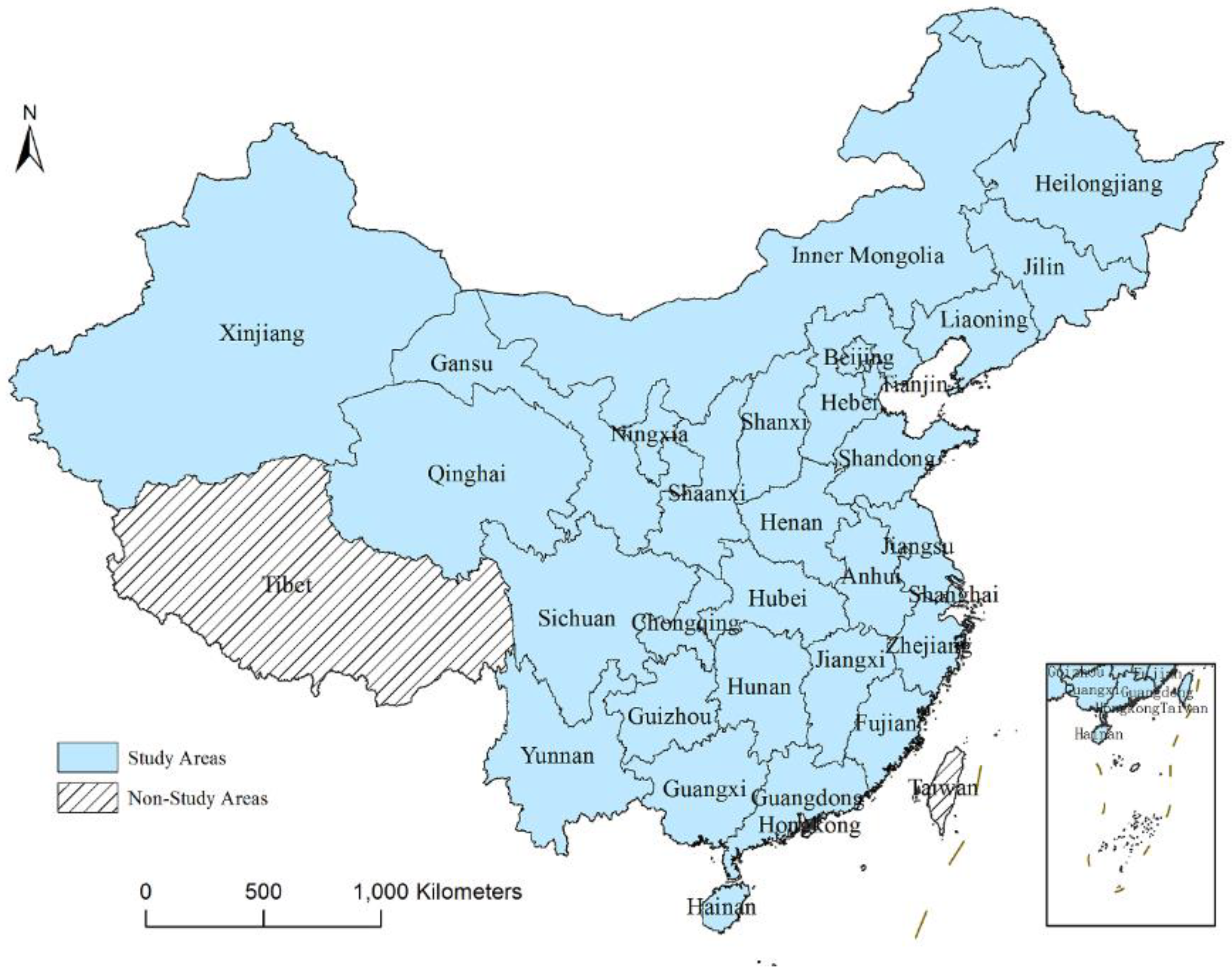
35]. Due to the unbalanced development of EFs and social factors in China’s 30 provinces, the heterogeneous characteristics of the restraining factors of the provincial EFs of China from 2003 to 2015 under different threshold variables were evaluated. This study has the following objectives: (1) the threshold effect of restraining factors on China’s provincial EFs will be explored under the variable of urbanization; (2) the heterogeneity of the EKC effect will be tested to identify whether there is a threshold effect of social factors on the inverted-U relationship between the EF and economic growth; (3) specific provincial heterogeneity will be analyzed and policy implications will be presented. To achieve these objectives, this article is presented as follows:
Section 2 reviews the literature on EKC and EF’s restraining factors.
Section 3 introduces the study areas, EF accounting and the threshold panel regression model.
Section 4 presents the results of the case study and analyzes the result of the factors affecting China. The final section summarizes the case study, gives policy implications, and provides limitations and directions for future research.
2. Literature Review
As discussed in the introduction, most studies on the factors associated with environmental impacts have focused on carbon emissions and economic growth [
36], whereas only a few of these studies have used the EF instead of carbon emissions in this scope. As an effective ecological model, EF analysis and accounting are widely used in environmental impact measurement [
20,
37], sustainability evaluations [
38], and policy making and planning [
27,
39]. Identifying the factors that restrain decreases in the EF is important when the driving factors, such as population growth, cannot be easily reduced in the short term. Thus, we have reviewed literature on the factors that impact EFs and highlighted the restraining (negative) factors for the EF. The literature on the restraining or influencing factors of the EF are listed in
Table 1, which shows that most of the studies on the relationship between social factors and EF are analyzed based on the EKC model; moreover, STIRPAT (stochastic impacts by regression on population, affluence, and technology), which was proposed by Dietz and Rosa [
40], could be used in conjunction with the EKC for a factor analysis.
Based on the literature listed in
Table 1, valid restraining factors for EFs were identified except the square of the economic term. Danish and Wang [
20] used the MG-CGE (Mean Group for Common Correlated Effects) for 11 newly industrialized countries and found that economic growth and urbanization had a moderating effect on the EF. The heterogeneity of the social factors that restrain the EF was also explored. Solarin and Al-Mulali [
34] explored the effect of the FDI (foreign direct investment) and urbanization on EF evolution for two types of countries and found that FDI and urbanization were restraining factors of the EF for developed countries. Long, Ji and Ulgiati [
33] found that the tertiary industry proportion and urbanization were restraining factors for EFs using panel data of 72 countries from 1998 to 2008. Ahmed et al. [
41] confirmed the restraining effect of export and foreign direct investment. Similarly, Al-mulali et al. [
32] identified financial development, trade openness and urbanization as restraining factors of EFs.
The main idea of the EKC hypothesis is that when the economy develops into a certain high level, environmental pollution tends to be reduced with the increasing economy, namely an inverted-U curve relationship between population and GDP. There are different viewpoints and research paths concerning EKC theory. Regarding the existence of the curve, ecological modernization theory (EMT) believed that with economic and social development, economic development has the ability to overcome ecological and environmental problems, and a curve will emerge. While the pessimistic theory of eco-environment believes that with the development of the social economy, the damage degree of ecological environment will become more serious, and it doesn’t acknowledge the existence of inverted-U curve. Regarding issues of the EKC examining model and empirical study, a lot of deficits were pointed out by Stern [
49], e.g., the premise of the hypothesis is too ideal; the model does not consider the feedback of environmental quality on production possibility nor the impact of trade on environmental degradation, therefore the model will underestimate the impact of economic development on the ecological environment [
49]. It is argued that most of the empirical study of EKC is weak in econometrics, due to the statistical flaws in the empirical data [
49]. The existence of pollution heaven [
50] would lead to the formation of the EKC relationship in the high-income countries by transferring embodied pollution to low-income countries. In spite of much controversy on EKC, there are still many meaningful empirical studies and policy implications [
36,
51].
For the literature related to the EF and the EKC hypothesis, the empirical results could be divided into three types based on the inverted-U relationship. First, the existence of an inverted-U relationship is not supported in a few research studies. Jia et al. [
42] used STIRPAT to analyze the factors of Henan’s EF from 1983 to 2006 using the PLS (partial least squares) method to eliminate multicollinearity and they found that an inverted-U relationship did not occur in Henan. Boutaud et al. [
43] investigated 131 countries in 2001 using a scatter plot and did not find an inverted-U relationship. Aşıcı and Acar [
44] and Bagliani et al. [
45] drew similar conclusions in their empirical research. Caviglia-Harris et al. [
9] and Aydin et al. [
46] also generated similar results in terms of the gross EF; however, they found that the EKC had an effect on components of the EF, with an inverted-U relationship observed between non-energy EF and GDP by Caviglia-Harris et al. and between fishing ground EF and GDP by Aydin et al.
Second, a few researchers support the existence of an inverted-U relationship for all of their study data. Aşıcı and Acar [
31] used panel data for 116 countries from 2004 to 2008 to verify the inverted-U relationship between EF and per capita income and a significant EKC was confirmed, and environmental regulation and governance were found to significantly improve the turning point of the EF. Destek and Sarkodie [
10] used AMG (augmented mean group) to investigate 11 newly industrialized countries from 1977 to 2013 by separate regressions and they found that accelerating economic growth and urbanization would be helpful for reducing the EF in the study area.
Finally, a few researchers tested the EKC hypothesis by groups according to the income level, urbanization level, etc. to determine the heterogeneity of the existence of the EKC. The inverted-U relationship was supported partially or heterogeneously. Al-mulali et al. [
32] divided the major global countries into four categories according to income level and found that the relationship between the square of GDP and ecological footprint varied for different income levels. Specifically, middle- and high-income countries exhibited this type of inverted-U relationship. Ulucak and Bilgili [
47] employed the CUP-FM (continuously updated fully modified) and CUP-BC (updated bias corrected) to explore the EKC and confirmed the EKC in all countries for three income levels; however, the EKC turning points were varied.
In addition, Liu et al. [
48] used the LMDI (logarithm mean decomposition index) to decompose the factors underlying Beijing’s EF for 2005 and 2010, although they did not identify restraining factors in their study.
Overall, some of the reviewed literature above studied the factors that influence EFs and identified a limited number of restraining factors on EF evolution. A few studies focused on the heterogeneity of the restraining factors and inverted-U relationship based on separate regressions by group. However, most of studies were not dedicated to the restraining factors, and the identification of the heterogeneity in the relationship between the restraining factors and EKC is limited. The essential restraining factors on EFs and associated heterogeneity must be determined to achieve urban sustainable development in a differentiated way during its developing stage.
4. Results and Analysis
4.1. Results of the Threshold Effect on EF Growth
According to the threshold regression models designed in the previous section, the existence of single-, double- and triple-threshold effects of restraining (regime-dependent) variables were tested under the threshold variable of urbanization. The regime-dependent variables included technology, openness, industrial structure and energy efficiency, which were constructed in model 1, model 2, model 3 and model 4, respectively. These tests aim to determine the heterogeneity of the relationship between EF and each restraining factor among different intervals of urbanization, which were divided based on the threshold regression. According the F-statistics and P-values in
Table 3, urbanization had significant single-threshold effects in the four models, and all of the single-threshold tests passed the 5% significant test, indicating the necessity of nonlinear models. For the double and triple thresholds, all four models did not pass the significant test, which indicates that there is only one structural break of urbanization between EF and each restraining variable.
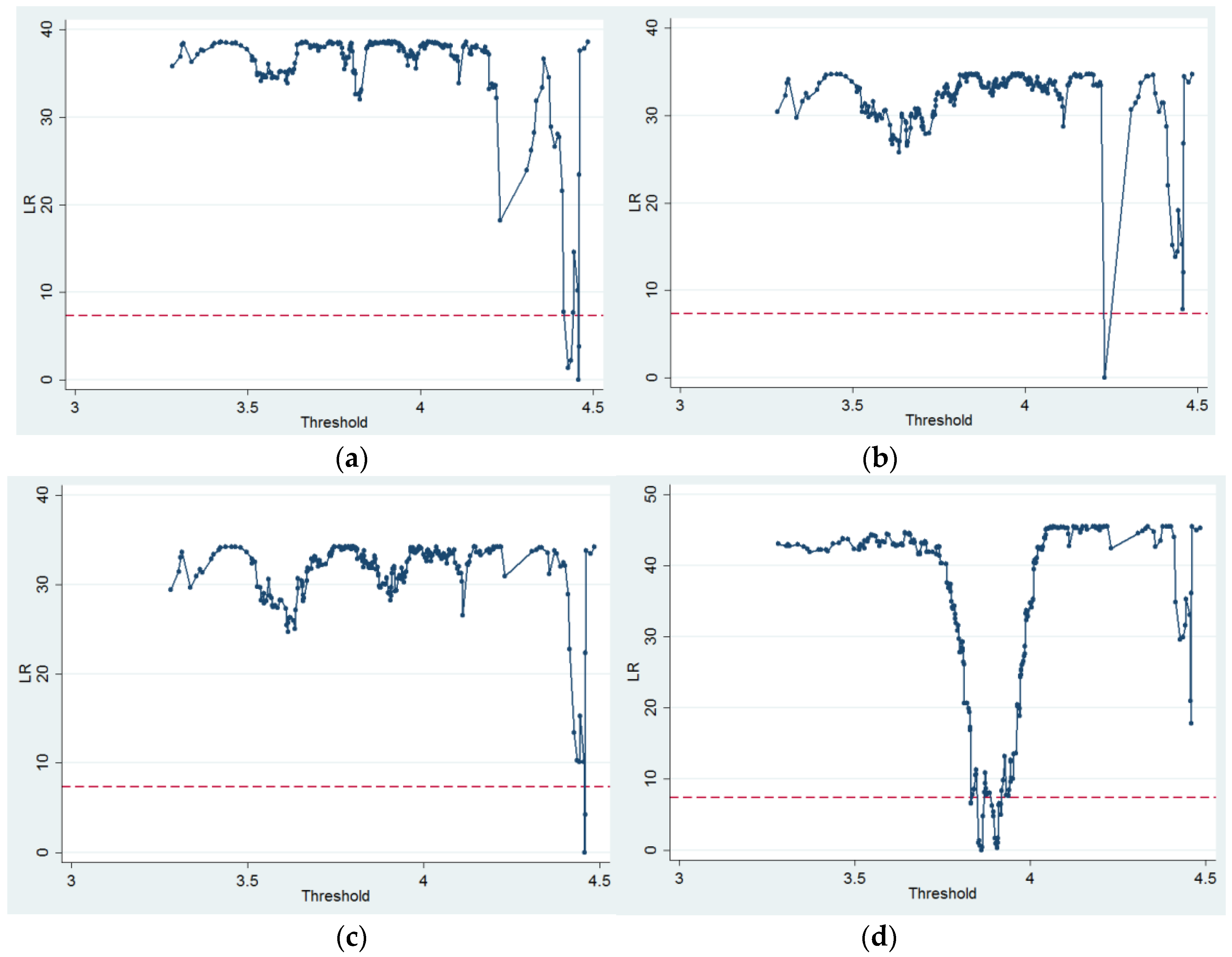
The likelihood ratio (LR) statistics for single-threshold estimates of urbanization in the four models are presented in
Figure 2, and sub-figures (a), (b), (c) and (d) present the LR statistics for single-threshold models from models 1 to 4. The red dashed lines in the sub-figures describe the critical 95% confidence level value. The single-threshold estimates are the value of parameters that obtain a value of zero for the LR statistic [
52].
Table 4 shows the threshold estimated value and corresponding urbanization rate for each regime-dependent variable. From model 1 to model 4, the single threshold estimated values of urbanization were 4.4567, 4.2299, 4.4567 and 3.8609, and the corresponding 95% confidence intervals were [4.4415, 4.4578], [4.2195, 4.2966], [4.4539, 4.4578] and [3.8532, 3.8628], respectively.
The results of the threshold regression coefficients from model 1 to model 4 are presented in
Table 5. In model 1, the coefficient of technology was −0.0237 in the urbanization rate interval that is no more than 86.2%, which did not pass the significant test. When urbanization exceeded the threshold, the coefficient exhibited a jumping change to −0.1098, which is significant at the confidence level of 1%. The threshold effect of technology indicates that the restraining effect is significant and enhanced only when the urbanization rate exceeds 86.2% for China’s 30 provinces. The jumping change in the coefficients for industrial structure is similar to that for technology. In model 3, the coefficient of industrial structure increased from −0.1 to −0.1588, which represents an increase from not significant to significant at the level of 5%. Model 1 and model 3 shared the same threshold value of urbanization, which indicates the synchronicity on EF reduction for the two restraining factors. The coefficients of foreign capital openness present considerable changes between the two intervals of urbanization in model 2, with the values increasing from −0.061 at a significance level of 1% to −0.3504 at the significance level of 1%. The change indicates that the restraining effect of foreign capital investments becomes much greater when urbanization exceeds the threshold of 68.71%. The situation is similar for energy efficiency in model 4, and the coefficients changed from −0.4762 (lnU ≤ 3.8609) with a significance level of 1% to −0.5788 (lnU > 3.8609) with a significance level of 1%. The restraining effect of energy efficiency was enhanced slightly when the urbanization rate exceeded the threshold 47.51% in model 4. The urbanization factor played a heterogeneous role in the EF reduction effect of each restraining factor. From low levels to high levels of urbanization, the role of technology, openness, industrial structure and energy efficiency in restraining EF growth was enhanced more or less significantly.
4.2. Results of the Threshold Effect on EKC
Table 5 shows that the coefficients of the square term of affluence were not significant and were negative simultaneously in the four models, which means that the EKC hypothesis cannot be significantly confirmed for the overall panel data. To further study the specific social conditions for the formation of an EKC between EF growth and economic development, as discussed in
Section 3, we constructed four models with different threshold variables based on model 1 to study the heterogeneity in the formation of the EKC hypothesis.
Table 6 shows the single-, double- and triple-threshold effects of the square term under the threshold variables of urbanization, openness, industrial structure and energy efficiency, which correspond to model 5, model 6, model 7 and model 8, respectively. The results show that openness, industrial structure and energy efficiency have significant single-threshold effects at the significance level of 5% according to the F-statistics and P-values in
Table 6. Meanwhile, the threshold variable openness passes the 10% significant test. All four models did not pass the significant test for the double- and triple-thresholds tests, which indicates that only one threshold exists. The results denote that the heterogeneity that occured for the EKC and the panel data would be divided into two regimes, between which there are jumping changes for the support of the EKC hypothesis.
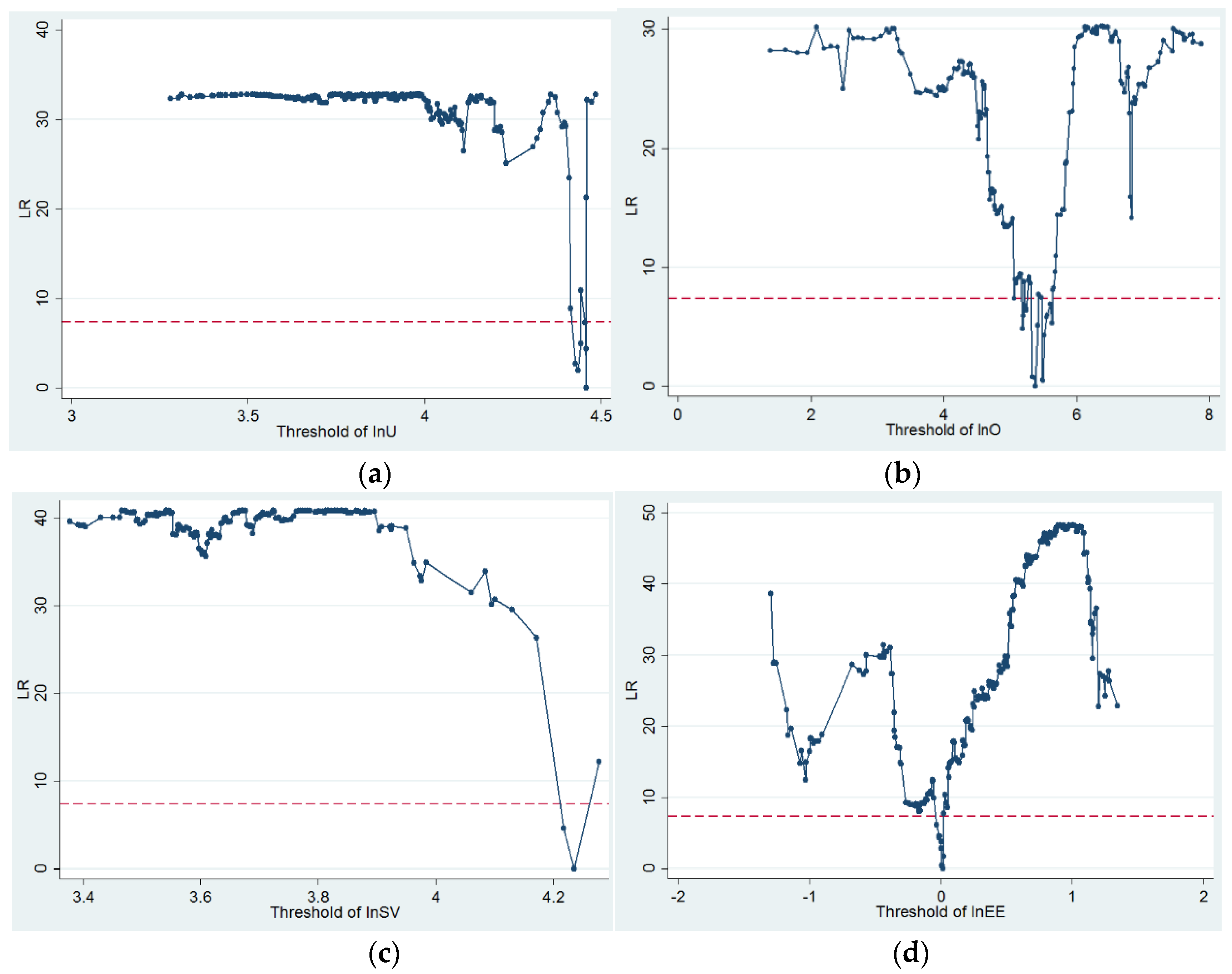
Following the test for the presence of a threshold effect, the LR statistic of the four models for single-threshold effect was performed and the LR results are presented in
Figure 3. The sub-figures (a), (b), (c) and (d) show the LR statistics for a single threshold from model 5 to model 8. As demonstrated in
Figure 2, the red dashed lines in the sub-figures describe the critical 95% confidence level value, and the single-threshold estimates are the values of the parameter that achieved a value of zero for the LR statistic.
Table 7 also shows the threshold estimated values and corresponding antilog values for the models. From model 5 to model 8, the single-threshold estimated values were 4.4567, 5.3706, 4.2356 and 0.0164, and the corresponding 95% confidence intervals were [4.4483, 4.4578], [5.3371, 5.4072], [4.1939, 4.2781] and [−0.0231, 0.0175], respectively.
Table 8 presents the threshold regression results on the formation of the EKC relationship between EF and affluence under the threshold variables of urbanization (model 5), openness (model 6), industrial structure (model 7) and energy efficiency (model 8). In model 5, the coefficient of the square term of affluence was −0.0132, which does not pass the significance test when the urbanization rate is no more than the threshold 86.2%. When urbanization exceeded the threshold, the coefficient exhibits a jumping change to −0.0872, which is significant at the confidence level of 1%. The coefficients of the square term in model 6 were 0.0662 and −0.0293 in the intervals before and after reaching the openness threshold of 214.99, respectively. When the per capita foreign capital investment exceeds the threshold for China’s provinces, the formation of the EKC tends to be supported at the significance level of 10%. The jumping change of the inverted-U relationship in model 7 is similar to the situation in model 5. The coefficient of the square term in model 7 changed from -0.021 with no significance to −0.1709 with significance at 1%. The significant turning point of the inverted-U relationship in model 7 is the optimal environmentally friendly evolution. As for the specific heterogeneity of the EKC relationship under the threshold variable energy efficiency in model 8, the coefficients of the square term changed from a positive value (0.131) to a negative value (−0.025) which is not statistically significant, indicating that the EKC relationship is not confirmed. Overall, the growth of the four social factors from low levels to high levels in the process of urbanization plays important roles in the EKC trends for the formation of the EF, and the orders of importance of the EKC formation trends could be industrial structure, urbanization, openness and energy efficiency, successively.
4.3. Analysis of the Heterogeneity of Restraining Factors Among China’s 30 Provinces
As shown in the analysis above, the four factors of technology, openness, industrial structure and energy efficiency played a more important role in restraining EF growth when the urbanization exceeded the corresponding threshold. It can be seen that accelerating urbanization promotes the role of these factors, and they each play a specific role. Technology progress is an effective way to reduce the ecological footprint intensity (EFI). Openness improvement brings foreign investment and further brings advanced technology and management, especially for China. Improving industrial structure (service sector’s proportion) is an effective way to restrain EF growth, as the low energy use and land use per GDP for the service sector and the EFI is much lower than that of primary sector or secondary industries. Following the threshold regressions from model 1 to model 4 above, all hypotheses of no single threshold were rejected, indicating significant threshold effects of technology, openness, industrial structure and energy efficiency on EF. China’s 30 provinces could be divided and analyzed to determine the specific heterogeneity based on the specific thresholds. The 30 provinces could be divided into two regimes by each threshold value from model 1 to model 4. The four models share the same threshold variable of urbanization, and the threshold values present a dispersed distribution from low to high. Hence, we divided the urbanization of China’s 30 provinces into four levels based on these threshold values as shown in
Table 9: low level, middle level, middle-high level and high level.
The interval of low-level urbanization was no more than 47.51%, and the provinces in the urbanization of this interval in 2015 (latest year in this study) were Guizhou, Gansu, Yunnan, Henan and Xinjiang. None of the factors had a high restraining effect on these provinces in this study. The interval of the middle level urbanization was more than 47.51% and no more than 68.7%, and the provinces that met the criteria included most of the provinces, e.g., Sichuan, Qinghai, Anhui, Hunan, Hebei, Jiangxi, Shaanxi, Shanxi, Hainan, Ningxia, Jilin, Hubei, Shandong, Heilongjiang, Inner Mongolia, Chongqing, Fujian, Zhejiang, Jiangsu, Liaoning and Guangdong. The initial years in which the provinces jumped to the middle level of urbanization varied. While Zhejiang, Jiangsu, Liaoning and Guangdong entered the middle level of urbanization before 2005, Sichuan, Qinghai, Anhui, Hunan, Hebei, Jiangxi and Shaanxi only jumped to this level after 2012. A comparison between the provinces at the middle level of urbanization and those at a low level of urbanization showed that energy efficiency plays a more restraining effect on the EF. Only one province-level city met the middle-high level of urbanization, i.e., Tianjin, and the value ranged from more than 68.71% to no more than 86.2%, and the initial year that this city jumped to the middle-high urbanization level occurred before 2003. With an urbanization rate of 82.64% in 2015, Tianjin will jump to the high level soon. When provinces enter the middle-high level of urbanization, in addition to energy efficiency, the openness begins to play a more important role in restraining EF growth compared with the previous two levels of urbanization which means that the per unit foreign capital investment will have a more restraining effect on the EF. Only Beijing and Shanghai were at the high level of urbanization, which requires a rate of more than 86.2%. As discussed, the same threshold value between technology and industrial structure indicates the close relationships among technology development, the service sector proportion and urbanization, and the two former factors play key roles in the threshold of the high-level urbanization. For the high level of urbanization, in addition to energy efficiency and openness, technology and industrial structure had a high restraining effect on the EF. The per unit technology improvement and increase in the service sector proportion would have a greater restraining effect on the EF in Beijing and Tianjin than other provinces. Due to the unbalanced development of urbanization in China, a heterogamous strategy should be made to restrain EF growth based on the results. For example, the EF restraining effect of technology and openness for the group of Beijing and Shanghai was 4.63 and 5.64 times that of other provinces.
As discussed above, the urbanization rate, openness and industrial structure have a threshold effect on the existence of the EKC for the EF of China’s 30 provinces, and only model 5 and model 7 exhibited a significant inverted−U relationship at the level of 1% when the urbanization and service sector proportion exceeded 86.2% and 69.1%, respectively. Beijing and Tianjin exhibited an inverted-U relationship in consideration of the threshold effect of urbanization, while only Beijing met the service sector proportion criterion of more than 69.1% that supports the EKC with a lower turning point. If the support for the EKC at the significance of 10% in model 6 is considered, then provinces with openness values that exceed the threshold will exhibit an inverted-U relationship to a certain degree, and they include Anhui, Henan, Hebei, Hubei, Sichuan, Chongqing, Jiangxi, Tianjin, Fujian, Shandong, Liaoning, Zhejiang, Beijing, Guangdong, Shanghai and Jiangsu. The EF of Beijing would reach the turning point the earliest, followed by Shanghai, Tianjin and parts of provinces at the middle level of urbanization. The order of provinces is consistent with the urbanization level order from high, middle-high to middle, which indicates that the urbanization rate has a positive effect on the formation tendency of the inverted-U relationship.
5. Conclusions and Policy Implications
5.1. Conclusions
This paper aimed to study the heterogeneity of the relationship between China’s 30 provincial EFs and associated restraining factors and explore the inverted-U relationship to improve the measures for the sustainable development of urbanization in China. For this purpose, a panel threshold regression and STIRPAT were used to explore the threshold effect on the restraining factors of EFs and the formation of the EKC based on provincial data in China from 2003 and 2015. The main conclusions are as follows:
(1) The threshold effects of the technology level, openness, industrial structure (service sector proportion) and energy efficiency on the EF are all significant and have values of 86.2%, 68.71%, 86.2% and 47.51%, respectively. From a low level to high level across the threshold values, the restraining effects of the four factors were all enhanced, and the jumping character of the restraining effect of openness was the largest. Technology level and industrial structure had the same threshold, which indicates their synchronicity in reaching a high restraining effect on the EF. The distribution of the four thresholds indicates that multistage urbanization has a restraining role on the EF based on different factors. As the urbanization level increases, more social factors have a high restraining effect on the EF.
(2) Urbanization and industrial structure have a statistically significant threshold effect on the formation of the inverted-U relationship between EF and affluence for China’s 30 provinces. The inverted-U turning point will form the earliest when the threshold of industrial structure exceeds 68.71%. The improvement of the urbanization rate not only promotes the formation of the inverted-U relationship but also effectively reduces the EF.
(3) The urbanization of China’s 30 provinces could be divided into four levels, namely, low level (U ≤ 47.51%), middle level (47.51% < U ≤ 68.71%), middle-high level (68.71% < U ≤ 86.20%) and high level (U > 86.20%). Most of the provinces are in the low and middle level, Tianjin is in the middle-high level, and Beijing and Shanghai are in the high level. High restraining effects of all four restraining factors are only observed in Beijing and Shanghai, where a statistically significant inverted−U relationship is supported as well.
(4) The threshold model is an effective way to capture the jumping character of the relationship between EF and its restraining factors. Analysis of the threshold effect is a valid way to study the heterogeneous relationship. This study contributes to the construction of econometric models to identify the heterogeneity of restraining factors and the EKC hypothesis of EF in China. The threshold models could be applied on a global scale or on other pollution indicators.
5.2. Policy Implications
Based on the empirical study and the conclusions above, three changes can be implemented to improve the restraining effects on the EF.
(1) The focus on improving technology, receiving foreign capital investments, optimizing the industrial structure and increasing energy efficiency should be phased according to the present urbanization levels of China’s 30 provinces. For provinces at the middle level of urbanization, including Sichuan, Qinghai, Anhui, Hunan, Hebei, Jiangxi, Shaanxi, Shanxi, Hainan, Ningxia, Jilin, Hubei, Shandong, Heilongjiang, Inner Mongolia, Chongqing, Fujian, Zhejiang, Jiangsu, Liaoning and Guangdong, the measures to increase energy efficiency should be a priority. Receiving foreign capital investments should be highlighted for Tianjin at the middle-high level of urbanization. In addition to the two previous points, Beijing and Shanghai should strengthen the restraining effect of technology progress and industrial structure optimization.
(2) For the sustainable development of the inverted-U relationship between EF and economic growth, Shanghai should strengthen the service sector proportion to achieve an optimized EKC tendency. To advance the formation of this tendency, foreign capital investment should be enhanced for Anhui, Henan, Hebei, Hubei, Sichuan, Chongqing, Jiangxi, Tianjin, Fujian, Shandong, Liaoning, Zhejiang, Beijing, Guangdong, Shanghai and Jiangsu.
(3) As an increasing urbanization level would promote the restraining effect of other social factors directly or indirectly, provinces at urbanization levels from low to middle-high should accelerate the urbanization process. Based on the above changes, each province would achieve sustainable development in turn.


