Evaluation of Prevalence of the Sarcopenia Level Using Machine Learning Techniques: Case Study in Tijuana Baja California, Mexico


Abstract
1. Introduction
2. Materials and Methods
2.1. Sample Size
2.2. Database
2.3. Machine Learning Models
Model Classification
3. Results
3.1. Significant Variables
3.2. Final Results
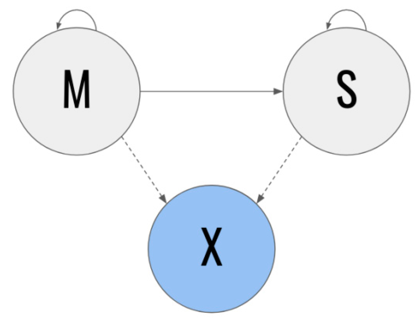
- Q: the set of states, Q = {s1, s2}, where s1 = M and s2 = S;
- A = {aij}: state transition matrix
- o
- aij = P (qt + 1 = sj | qt = si);
- B = {bj(k)}: State emission probability j
- o
- bj(k) = P (k en t | qt = sj);
- π = {πi}: initial distribution
- o
- πi = P (q0 = si).
3.2.1. Sodium
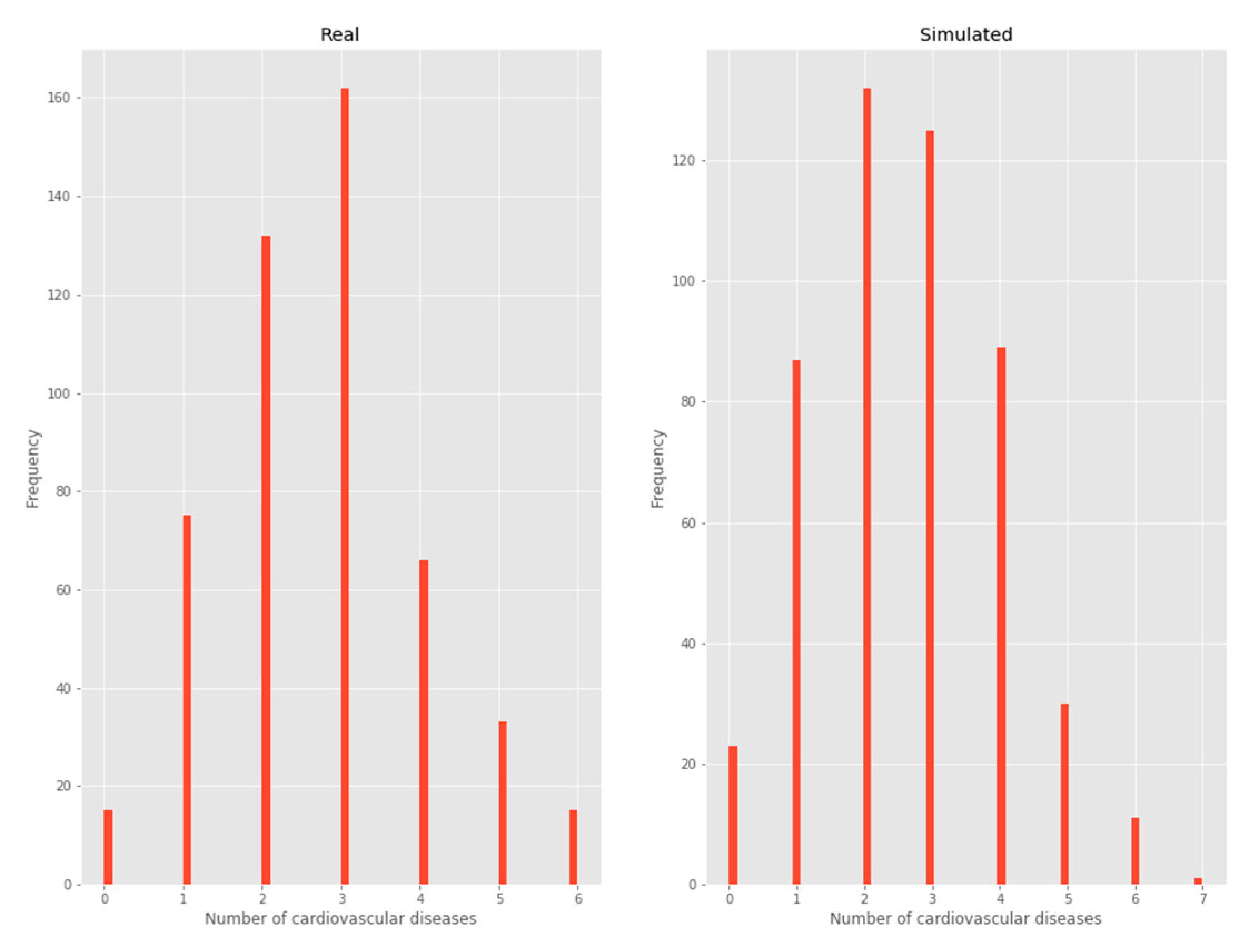
3.2.2. Number of chronic diseases
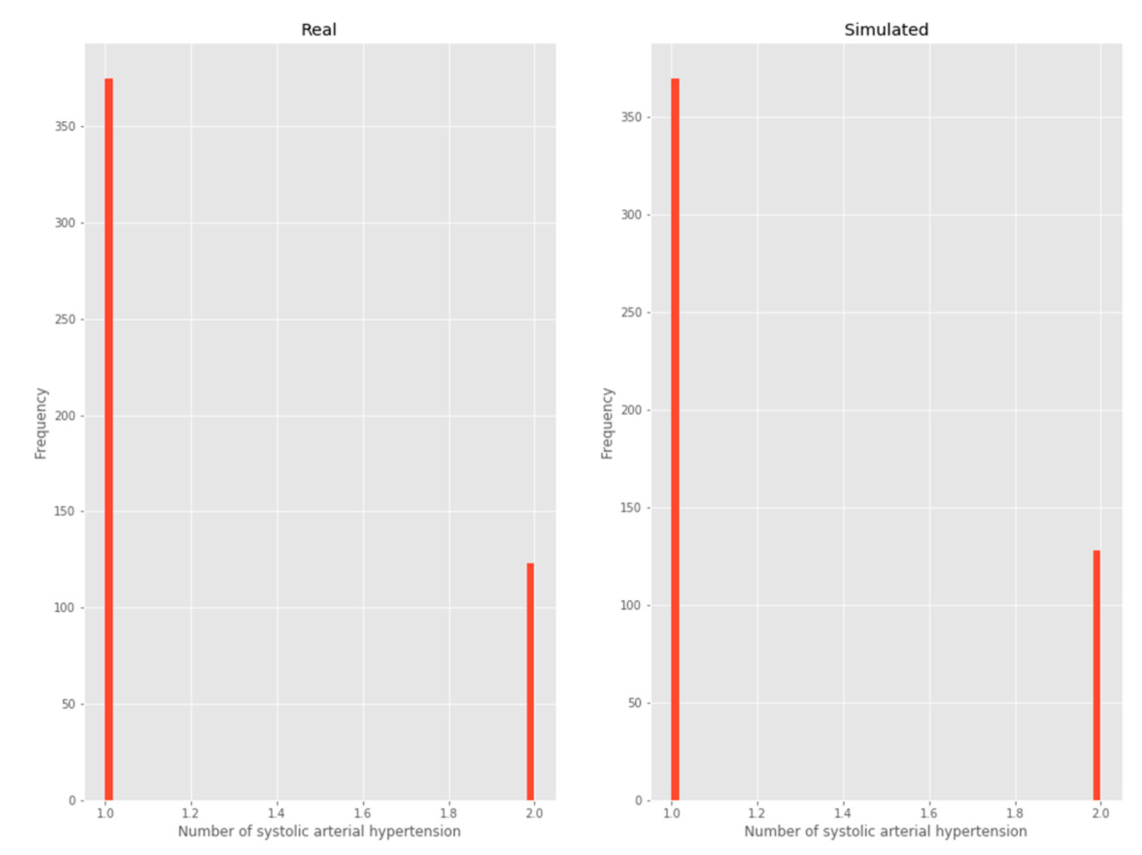
3.2.3. Systolic arterial hypertension
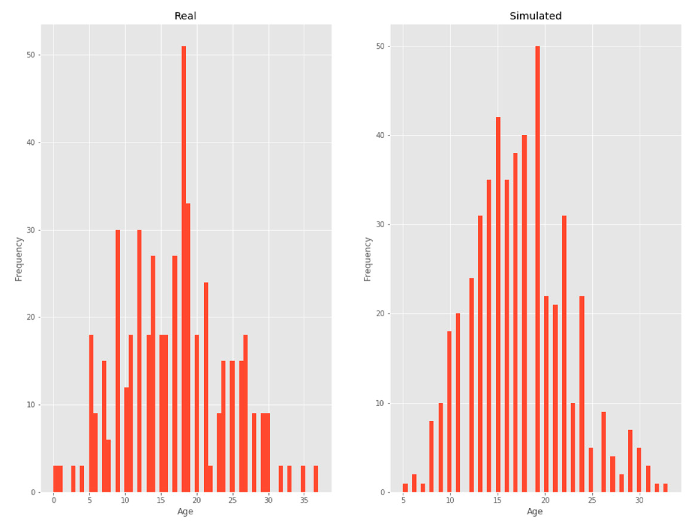
3.2.4. Age
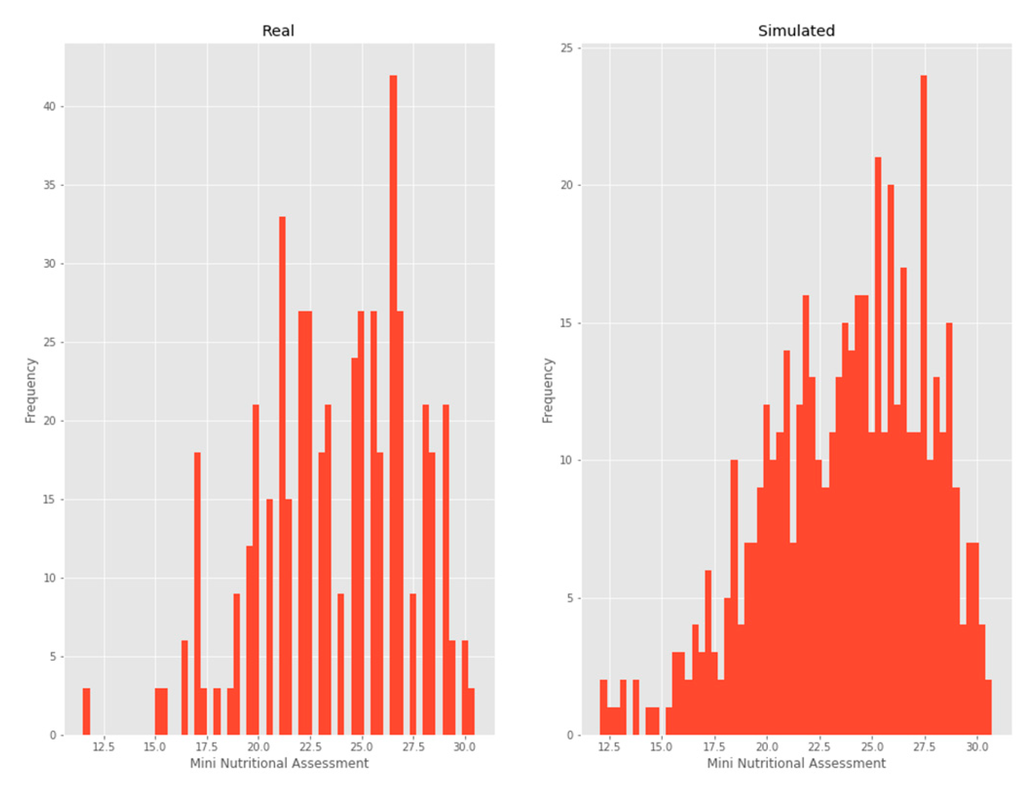
3.2.5. MNA
4. Discussion
5. Conclusions
Author Contributions
Funding
Acknowledgments
Conflicts of Interest
References
- Espinel-Bermúdez, M.C.; Sánchez-García, S.; García-Peña, C.; Trujillo, X.; Huerta-Viera, M.; Granados-García, V.; Arias-Merino, E.D. Associated factors with sarcopenia among Mexican elderly: 2012 National Health and Nutrition Survey. Rev. Médica Del Inst. Mex. Del Seguro Soc. 2018, 56, 46–53. [Google Scholar]
- Van Ancum, J.M.; Scheerman, K.; Jonkman, N.H.; Smeenk, H.E.; Kruizinga, R.C.; Meskers, C.G.; Maier, A.B. Change in muscle strength and muscle mass in older hospitalized patients: A systematic review and meta-analysis. Exp. Gerontol. 2017, 92, 34–41. [Google Scholar] [CrossRef]
- Martone, A.M.; Bianchi, L.; Abete, P.; Bellelli, G.; Bo, M.; Cherubini, A.; Marzetti, E. The incidence of sarcopenia among hospitalized older patients: Results from the Glisten study. J. Cachexia Sarcopenia Muscle 2017, 8, 907–914. [Google Scholar] [CrossRef]
- Dreder, A. Machine Learning Based Approaches for Identifying Sarcopenia-Related Genomic Biomarkers in Ageing Males; Northumbria University: Newcastle, UK, 2017; Available online: http://nrl.northumbria.ac.uk/36184/ (accessed on 11 December 2019).
- Hamrioui, S.; de la Torre Díez, I.; Garcia-Zapirain, B.; Saleem, K.; Rodrigues, J.J.P.C. A Systematic Review of Security Mechanisms for Big Data in Health and New Alternatives for Hospitals. Wirel. Commun. Mob. Comput. 2017, 2017, 6. [Google Scholar] [CrossRef]
- Michael, B. Machine Learning in Python: Essential Techniques for Predictive Analysis; John Wiley & Sons, Inc.: Hoboken, NJ, USA, 2015. [Google Scholar]
- Alonso, S.G.; de la Torre Diez, I.; Zapirain, B.G. Predictive, Personalized, Preventive and Participatory (4P) Medicine Applied to Telemedicine and eHealth in the Literature. J. Med. Syst. 2019, 43, 140. [Google Scholar] [CrossRef]
- Mugueta-Aguinaga, I.; Garcia-Zapirain, B. Is Technology Present in Frailty? Technology a Back-up Tool for Dealing with Frailty in the Elderly: A Systematic Review. Aging Dis. 2017, 8, 176–195. [Google Scholar] [CrossRef] [PubMed]
- De la Torre, I.; Cosgaya, H.M.; García-Zapirain, B.; López-Coronado, M. Big data in health: A literature review from the year 2005. J. Med. Syst. 2016, 40, 209. Available online: https://www.ncbi.nlm.nih.gov/pubmed/27520614 (accessed on 23 December 2019). [CrossRef] [PubMed]
- Lupianez-Villanueva, F.; Anastasiadou, D.; Codagnone, C.; Nuno-Solinis, R.; Garcia-Zapirain Soto, M.B. Electronic Health Use in the European Union and the Effect of Multimorbidity: Cross-Sectional Survey. J. Med. Internet Res. 2018, 20, e165. [Google Scholar] [CrossRef] [PubMed]
- Coplade, B.C. Tijuana, Baja California: COPLADE; 2017; p. 10. Available online: http://www.copladebc.gob.mx/publicaciones/2017/Mensual/Tijuana%202017.pdf (accessed on 23 December 2019).
- Castro, E.M.M. Bioestadística aplicada en investigación clínica: Conceptos básicos. Rev. Médica Clínica Las Condes. 2019, 30, 50–65. [Google Scholar] [CrossRef]
- Steffl, M.; Bohannon, R.W.; Sontakova, L.; Tufano, J.J.; Shiells, K.; Holmerova, I. Relationship between sarcopenia and physical activity in older people: A systematic review and meta-analysis. Clin. Interv. Aging 2017, 12, 835–845. [Google Scholar] [CrossRef] [PubMed]
- Liu, P.; Hao, Q.; Hai, S.; Wang, H.; Cao, L.; Dong, B. Sarcopenia as a predictor of all-cause mortality among community-dwelling older people: A systematic review and meta-analysis. Maturitas 2017, 103, 16–22. [Google Scholar] [CrossRef] [PubMed]
- Bianchi, L.; Abete, P.; Bellelli, G.; Bo, M.; Cherubini, A.; Corica, F.; Rossi, A.P. Prevalence and Clinical Correlates of Sarcopenia, Identified According to the EWGSOP Definition and Diagnostic Algorithm, in Hospitalized Older People: The GLISTEN Study. J. Gerontol. Ser. A 2017, 72, 1575–1581. [Google Scholar] [CrossRef] [PubMed]
- Polan, D.F.; Brady, S.L.; Kaufman, R.A. Tissue segmentation of computed tomography images using a Random Forest algorithm: A feasibility study. Phys. Med. Biol. 2016, 61, 6553–6569. [Google Scholar] [CrossRef] [PubMed]
- Cassia Braga, R. SciELO-Public Health-Name segmentation using hidden Markov models and its application in record linkage Name segmentation using hidden Markov models and its application in record linkage. Cad. De Saude Publica 2014, 30, 2039–2048. Available online: https://www.scielosp.org/scielo.php?script=sci_arttext&pid=S0102-311X2014001102039 (accessed on 22 January 2020).
- Hodinka, L. Sarcopenia, Frailty and Dismobility. Biomed. J. Sci. Tech. Res. 2018, 7, 5776–5779. Available online: https://biomedres.us/fulltexts/BJSTR.MS.ID.001472.php (accessed on 22 January 2020). [CrossRef]
- Walston, J.D. Sarcopenia in older adults. Curr. Opin. Rheumatol. 2012, 24, 623–627. [Google Scholar] [CrossRef] [PubMed]
- Burns, J.E.; Yao, J.; Chalhoub, D.; Chen, J.J.; Summers, R.M. A Machine Learning Algorithm to Estimate Sarcopenia on Abdominal CT. Acad. Radiol. 2020, 27, 311–320. [Google Scholar] [CrossRef]
- Lenchik, L.; Boutin, R.D. Sarcopenia: Beyond Muscle Atrophy and into the New Frontiers of Opportunistic Imaging, Precision Medicine, and Machine Learning. Semin. Musculoskelet Radiol. 2018, 22, 307–322. [Google Scholar] [CrossRef]
- Qian, D. Fully-automated Segmentation of Muscle Measurement on CT in Detecting Central Sarcopenia: A Trend of Standardization. Acad. Radiol. 2020, 27. Available online: https://www.academicradiology.org/article/S1076-6332(19)30597-5/abstract#articleInformation (accessed on 10 January 2020).
- Barnard, R.; Tan, J.; Roller, B.; Chiles, C.; Weaver, A.A.; Boutin, R.D.; Lenchik, L. Machine Learning for Automatic Paraspinous Muscle Area and Attenuation Measures on Low-Dose Chest CT Scans. Acad. Radiol. 2019, 26, 1686–1694. [Google Scholar] [CrossRef]
- Graffy, P.M.; Liu, J.; Pickhardt, P.J.; Burns, J.E.; Yao, J.; Summers, R.M. Deep learning-based muscle segmentation and quantification at abdominal CT: Application to a longitudinal adult screening cohort for sarcopenia assessment. Br. J. Radiol. 2019, 92, 20190327. [Google Scholar] [CrossRef] [PubMed]
- Cernea, A.; Fernández-Martínez, J.L.; de Andrés-Galiana, E.J.; Fernández-Muñiz, Z.; Bermejo-Millo, J.C.; González-Blanco, L.; Caballero, B. Prognostic networks for unraveling the biological mechanisms of Sarcopenia. Mech. Ageing Dev. 2019, 182, 111129. [Google Scholar] [CrossRef] [PubMed]
- Kang, Y.-J.; Yoo, J.-I.; Ha, Y.-C. Sarcopenia feature selection and risk prediction using machine learning: A cross-sectional study. Medicine 2019, 98, e17699. [Google Scholar] [CrossRef] [PubMed]
- Cui, M.; Gang, X.; Gao, F.; Wang, G.; Xiao, X.; Li, Z.; Wang, G. Risk assessment of sarcopenia in patients with type 2 diabetes mellitus using data mining methods. Front. Endocrinol. 2020, 3, 123. [Google Scholar] [CrossRef]


| Gender | MMI | Hand Grip Strength | Walking Speed | |
|---|---|---|---|---|
| Women | 65% | <6.1 kg/m2 | <20 | <0.8 |
| Men | 35% | <8.5 kg/m2 | <30 | <0.8 |
| Metric | Formula |
|---|---|
| Accuracy | |
| Precision | |
| F1 |
| DataSET 1 |
| Age, Systolic arterial hypertension, mini nutritional assessment (MNA), Number of chronic diseases, Sodium |
| DataSET 2 |
| Age, Systolic arterial hypertension, MNA, Number of chronic diseases, Sodium, Drugs, Lawton |
| DataSET 3 |
| Age, Systolic arterial hypertension, MNA, Number of chronic diseases, Sodium, Drugs, Lawton, Hb, Major neurocognitive disorder, Dementia, Occupation, Means of support |
| DataSET 4 |
| Status, Gender, Age, Level of education, Literacy, Civil status, Carer, Religion, Residence, Occupation, Economy, Means of support, Eyesight, Visual aid, Hearing, Hearing aid, Number of chronic diseases, Systolic arterial hypertension, Major neurocognitive disorder, PARKIN, HIPOT, HIPERT’, CANCER, COPD, Dyslipidemia, Chronic renal insufficiency, Other, Hepatic insufficiency, Smoking, Alcoholism, Drug use, Biomass exposure, MMSE, GDS, Depression, Barthel, Falls, Number of falls, Ulcers, Norton, Lawton, MNA, Charlson, Height in mts, Dementia, Cognition, Cerebrovascular disease, Infection, Pain, Cancer, Hb, Urea, Creatinine, Albumin, Glucose, ’Sodium’ |
| CLASSIFIERS | DataSET 1 | DataSET 2 | DataSET 3 | DataSET 4 | DataSET | ||||||||
|---|---|---|---|---|---|---|---|---|---|---|---|---|---|
| ACC | F1 | P | ACC | F1 | P | ACC | F1 | P | ACC | F1 | P | Final | |
| RBF SVM | 0.825 | 0.902 | 0.828 | 0.813 | 0.897 | 0.813 | 0.813 | 0.897 | 0.813 | 0.813 | 0.897 | 0.813 | 1, 2, 3, 4 |
| Decision Tree | 0.831 | 0.900 | 0.864 | 0.795 | 0.879 | 0.844 | 0.819 | 0.897 | 0.84 | 0.765 | 0.842 | 0.866 | 1, 3 |
| Random Forest | 0.825 | 0.901 | 0.836 | 0.825 | 0.902 | 0.827 | 0.795 | 0.886 | 0.810 | 0.801 | 0.89 | 0.811 | 1, 2, 4 |
| Linear SVM | 0.813 | 0.897 | 0.813 | 0.813 | 0.897 | 0.813 | 0.813 | 0.897 | 0.813 | 0.765 | 0.842 | 0.866 | 2, 3 |
| CLASSIFIERS | DataSET 1 | DataSET 2 | DataSET 3 | DataSET 4 | DataSET | ||||||||
|---|---|---|---|---|---|---|---|---|---|---|---|---|---|
| ACC | F1 | P | ACC | F1 | P | ACC | F1 | P | ACC | F1 | P | Final | |
| RBF SVM | 0.81 | 0.896 | 0.817 | 0.813 | 0.897 | 0.81 | 0.81 | 0.9 | 0.81 | 0.81 | 0.9 | 0.81 | 1, 2, 3, 4 |
| Decision Tree | 0.831 | 0.900 | 0.864 | 0.807 | 0.885 | 0.855 | 0.783 | 0.870 | 0.837 | 0.662 | 0.704 | 0.873 | 1 |
| Random Forest | 0.807 | 0.891 | 0.819 | 0.819 | 0.899 | 0.82 | 0.795 | 0.885 | 0.813 | 0.81 | 0.89 | 0.81 | 2, 4 |
| MPL | 0.84 | 0.905 | 0.855 | 0.783 | 0.870 | 0.853 | 0.747 | 0.844 | 0.839 | 0.716 | 0.817 | 0.842 | 1 |
| CLASSIFIERS | DataSET 1 | DataSET 2 | DataSET 3 | DataSET 4 | DataSET | ||||||||
|---|---|---|---|---|---|---|---|---|---|---|---|---|---|
| ACC | F1 | P | ACC | F1 | P | ACC | F1 | P | ACC | F1 | P | Final | |
| RBF SVM | 0.807 | 0.893 | 0.812 | 0.813 | 0.897 | 0.813 | 0.813 | 0.897 | 0.813 | 0.813 | 0.897 | 0.813 | 2, 3, 4 |
| Decision Tree | 0.825 | 0.895 | 0.867 | 0.789 | 0.872 | 0.852 | 0.753 | 0.848 | 0.825 | 0.656 | 0.701 | 0.868 | 1 |
| Random Forest | 0.789 | 0.880 | 0.816 | 0.801 | 0.886 | 0.813 | 0.813 | 0.896 | 0.817 | 0.813 | 0.897 | 0.813 | 3, 4 |
| Gaussian Process | 0.813 | 0.897 | 0.813 | 0.807 | 0.891 | 0.820 | 0.807 | 0.891 | 0.820 | 0.747 | 0.850 | 0.817 | 1 |
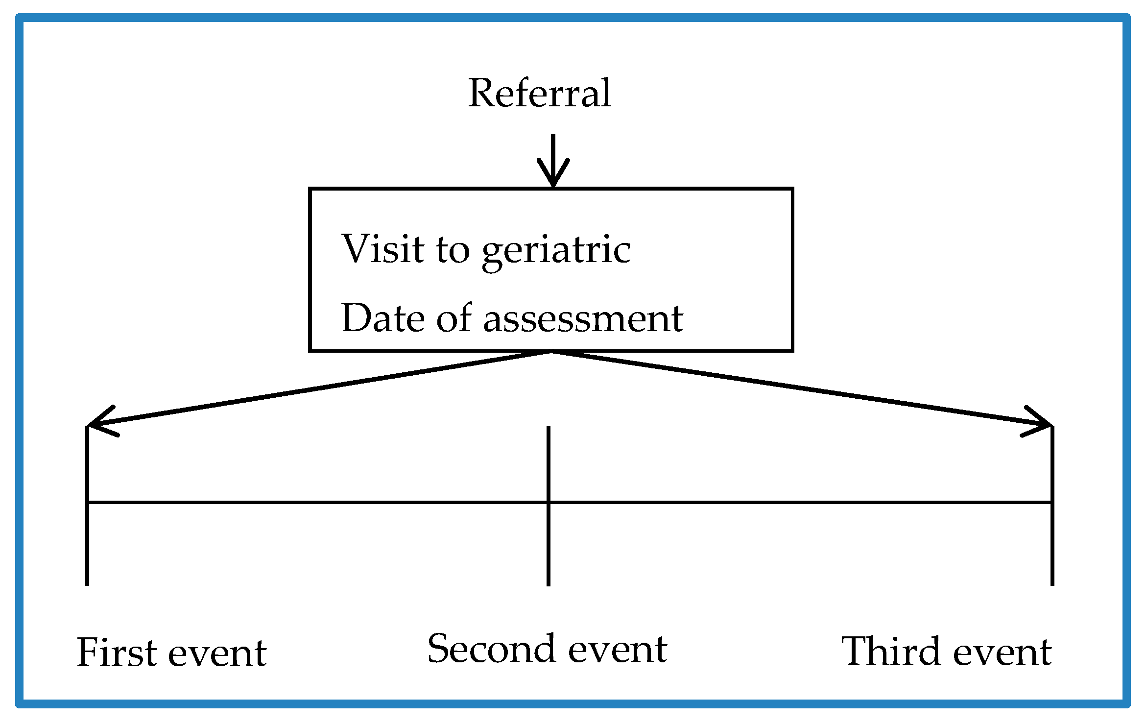
| CLASSIFIERS | DataSET 1—First Event | DataSET 1—Second Event | DataSET 1—Third Event | ||||||
|---|---|---|---|---|---|---|---|---|---|
| ACC | F1 | P | ACC | F1 | P | ACC | F1 | P | |
| Decision Tree | 0.831 | 0.900 | 0.864 | 0.831 | 0.900 | 0.864 | 0.825 | 0.895 | 0.867 |
© 2020 by the authors. Licensee MDPI, Basel, Switzerland. This article is an open access article distributed under the terms and conditions of the Creative Commons Attribution (CC BY) license (http://creativecommons.org/licenses/by/4.0/).
Share and Cite
Castillo-Olea, C.; Garcia-Zapirain Soto, B.; Zuñiga, C. Evaluation of Prevalence of the Sarcopenia Level Using Machine Learning Techniques: Case Study in Tijuana Baja California, Mexico. Int. J. Environ. Res. Public Health 2020, 17, 1917. https://doi.org/10.3390/ijerph17061917
Castillo-Olea C, Garcia-Zapirain Soto B, Zuñiga C. Evaluation of Prevalence of the Sarcopenia Level Using Machine Learning Techniques: Case Study in Tijuana Baja California, Mexico. International Journal of Environmental Research and Public Health. 2020; 17(6):1917. https://doi.org/10.3390/ijerph17061917
Chicago/Turabian StyleCastillo-Olea, Cristián, Begonya Garcia-Zapirain Soto, and Clemente Zuñiga. 2020. "Evaluation of Prevalence of the Sarcopenia Level Using Machine Learning Techniques: Case Study in Tijuana Baja California, Mexico" International Journal of Environmental Research and Public Health 17, no. 6: 1917. https://doi.org/10.3390/ijerph17061917
APA StyleCastillo-Olea, C., Garcia-Zapirain Soto, B., & Zuñiga, C. (2020). Evaluation of Prevalence of the Sarcopenia Level Using Machine Learning Techniques: Case Study in Tijuana Baja California, Mexico. International Journal of Environmental Research and Public Health, 17(6), 1917. https://doi.org/10.3390/ijerph17061917