Assessing the Influence of Socioeconomic Status and Air Pollution Levels on the Public Perception of Local Air Quality in a Mexico-US Border City

 ,
,  ,
,
Abstract
1. Introduction
1.1. Air Pollution in the Context of Sustainable Development
1.2. Air Quality Perception
2. Methods
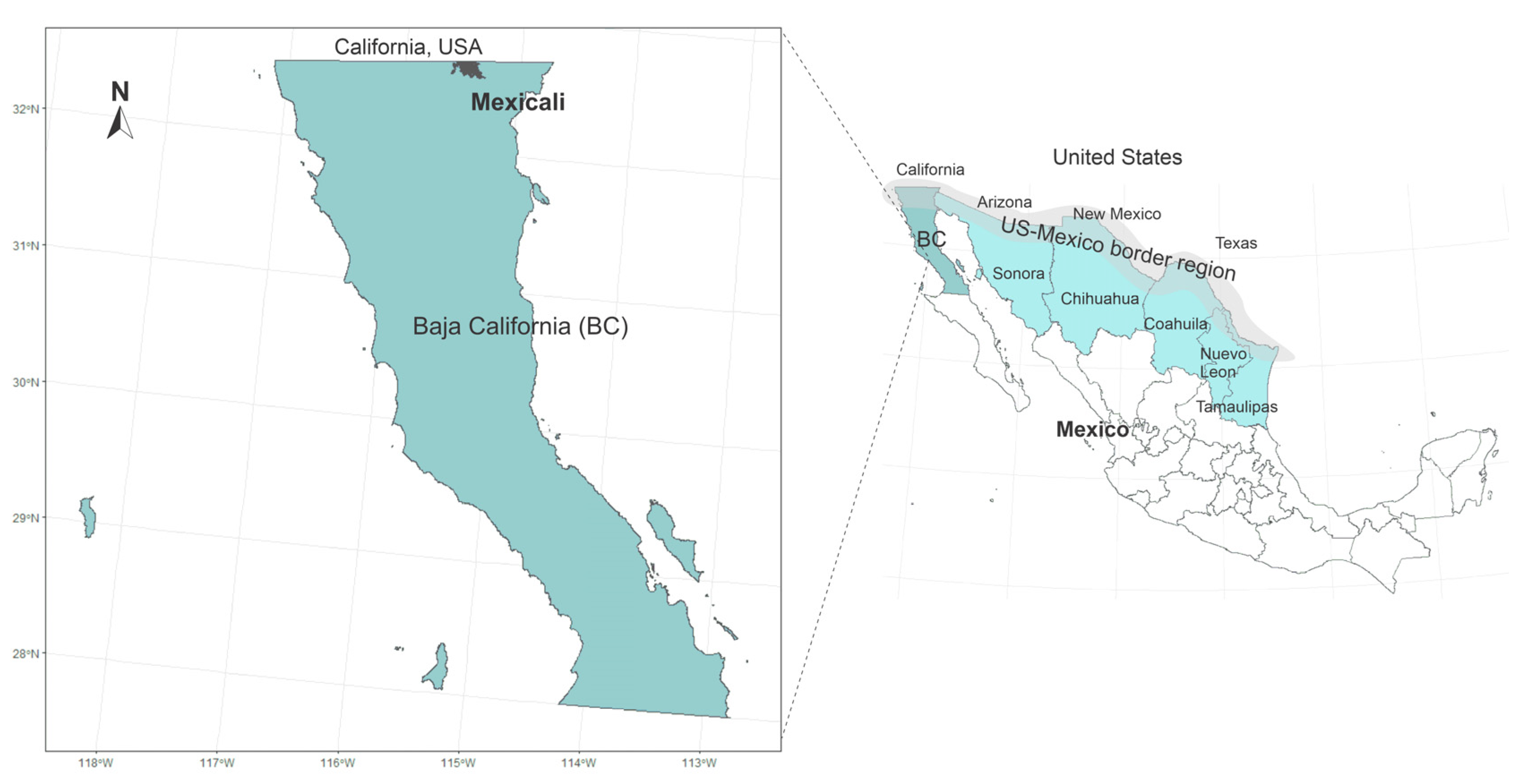
2.1. Study Site
2.2. Air Pollution Data and the Exposure Estimation Model
2.3. Social Vulnerability Index
2.4. Spatial Analysis
2.5. Data Collection and Statistical Models of Individual Socioeconomic Characteristics and Air Quality Perception
2.5.1. Data Collection from the Survey
2.5.2. Statistical Analysis
3. Results
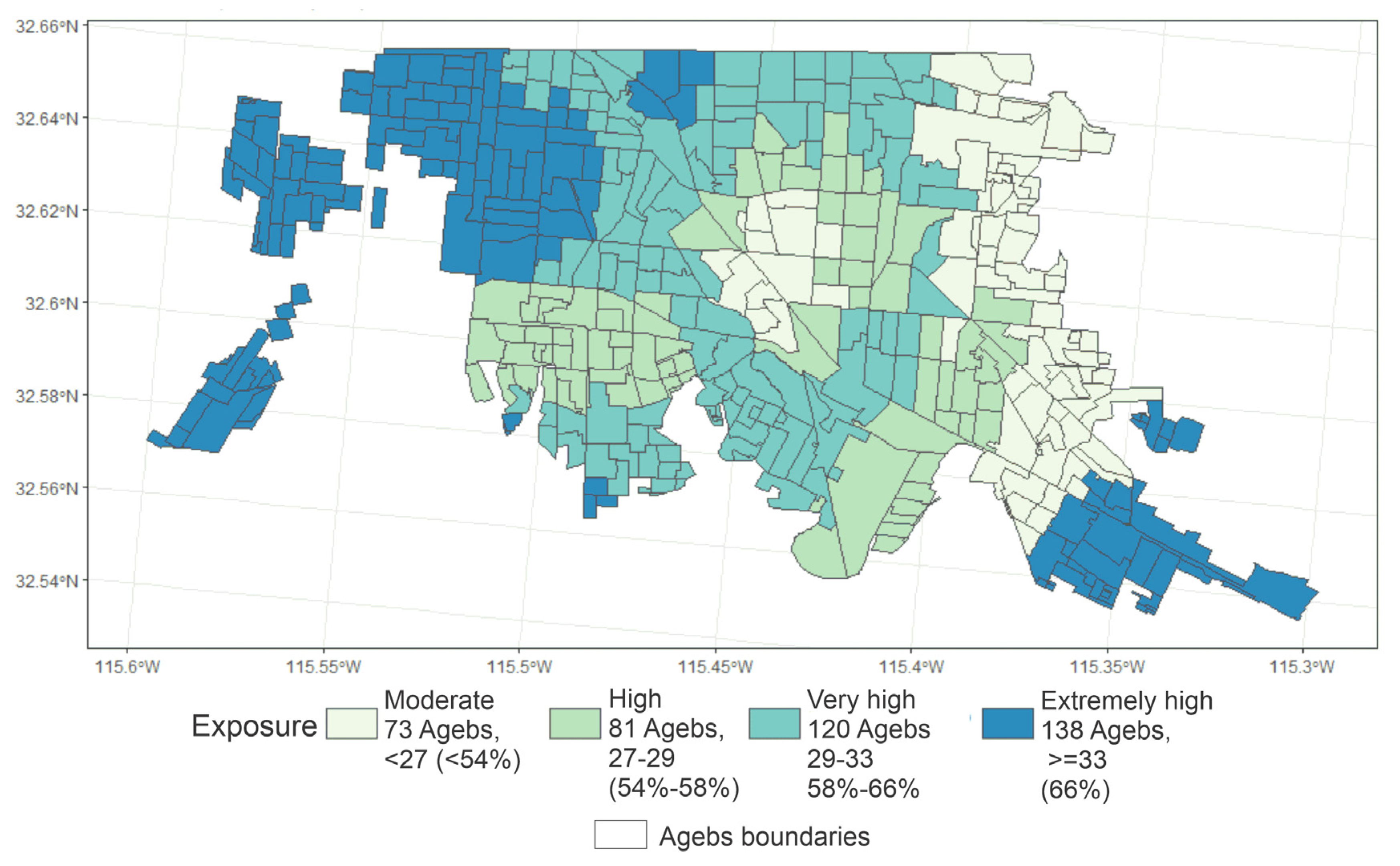
3.1. Estimation and Spatial Distribution of PM10 Exposure
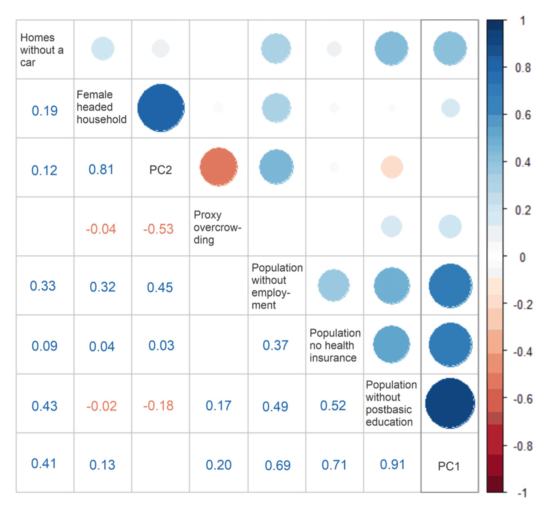
3.2. Estimation of Social Vulnerability
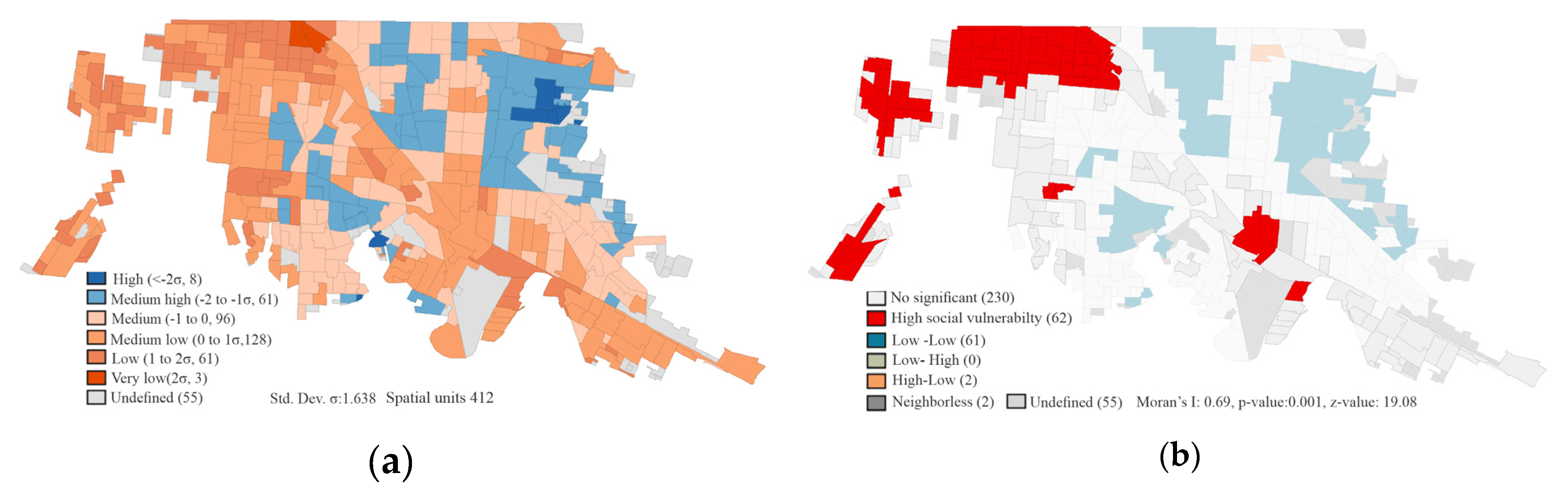
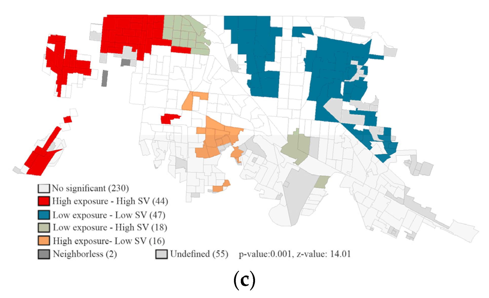
3.3. Spatial Distribution of Social Vulnerability and Autocorrelation with Estimated Exposure to PM10
3.4. Descriptive Statistics and Spatial Distribution of Air Quality Perception
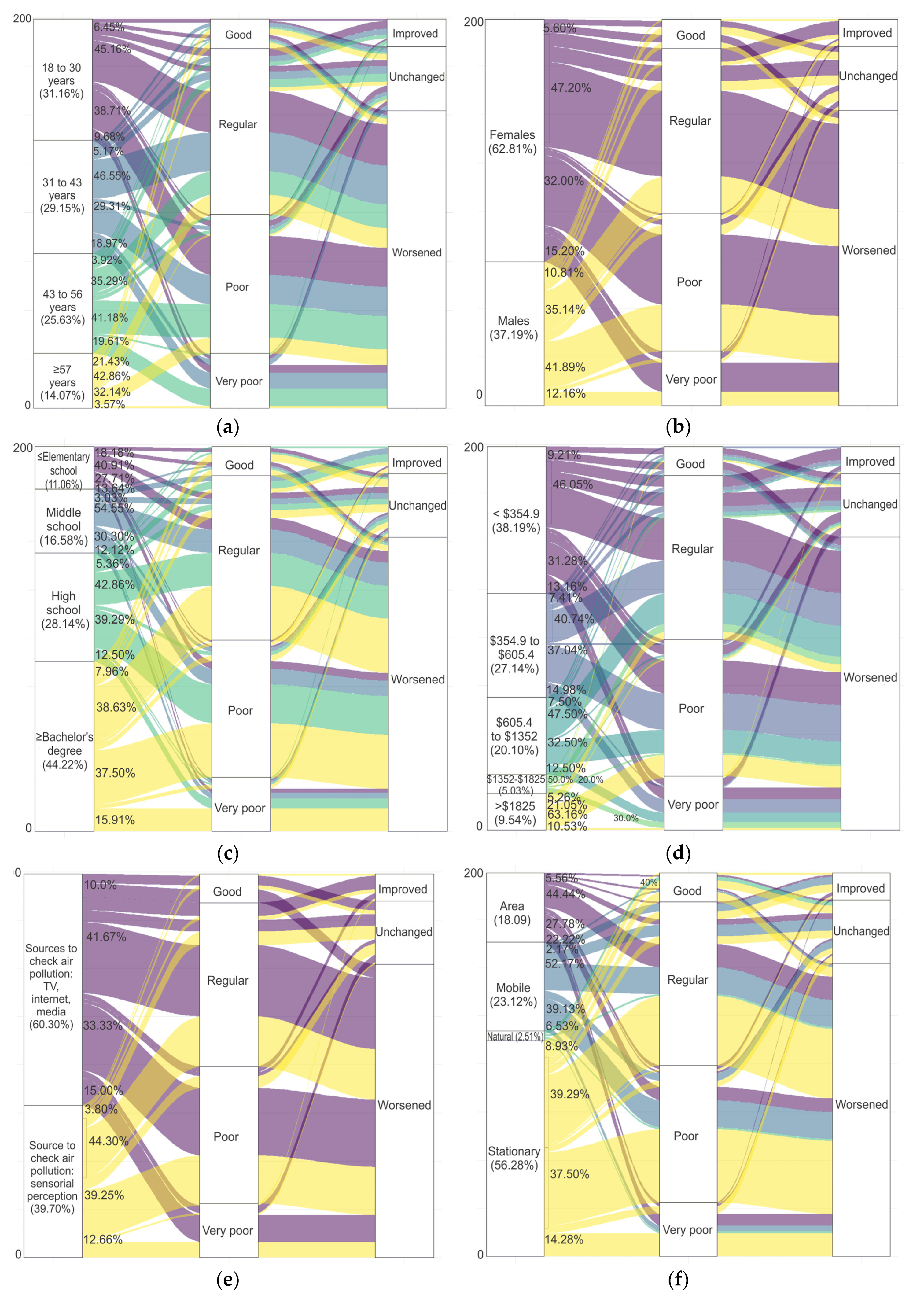
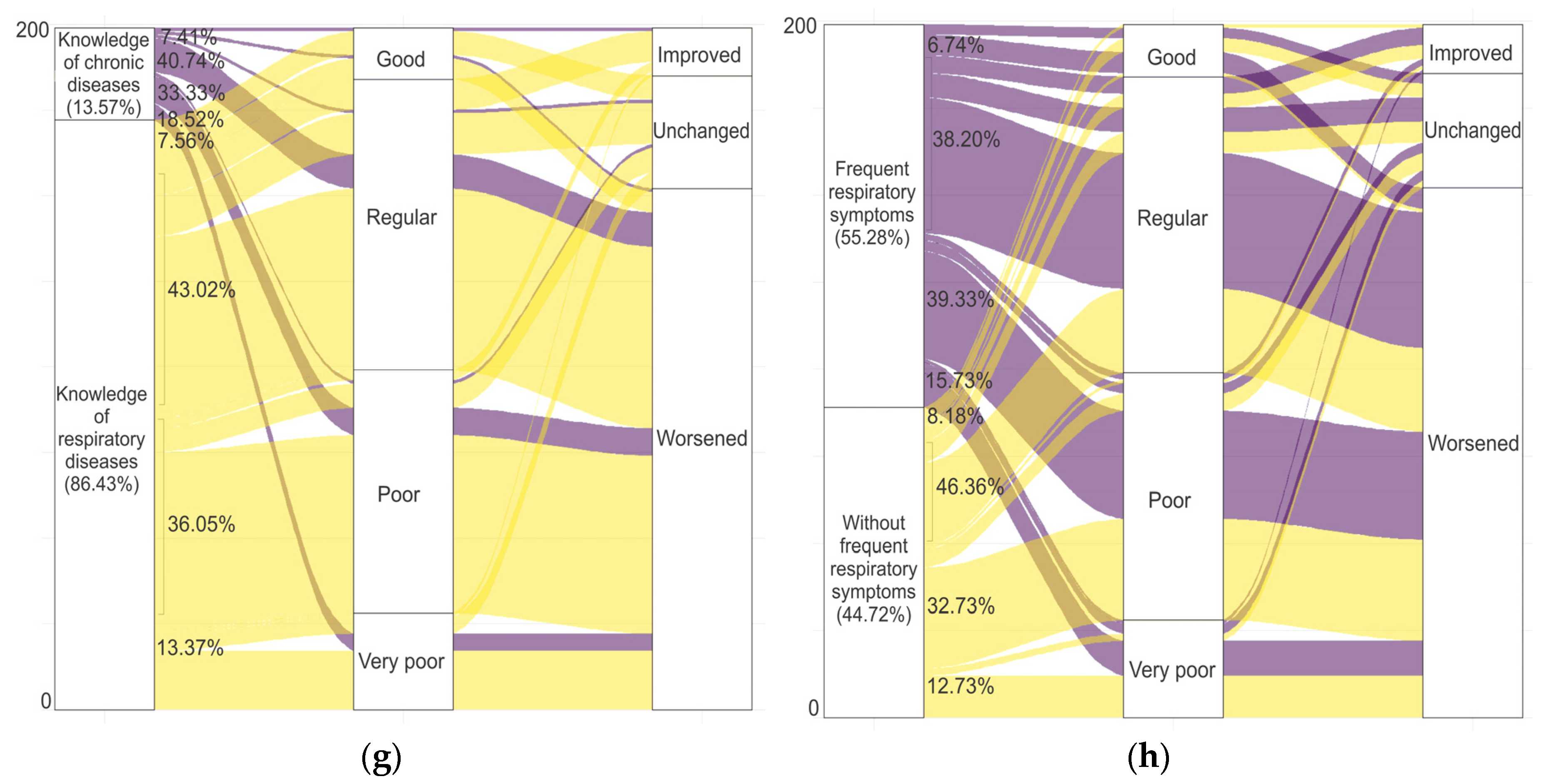
3.4.1. Description of Individual Responses by Air Quality Perceived
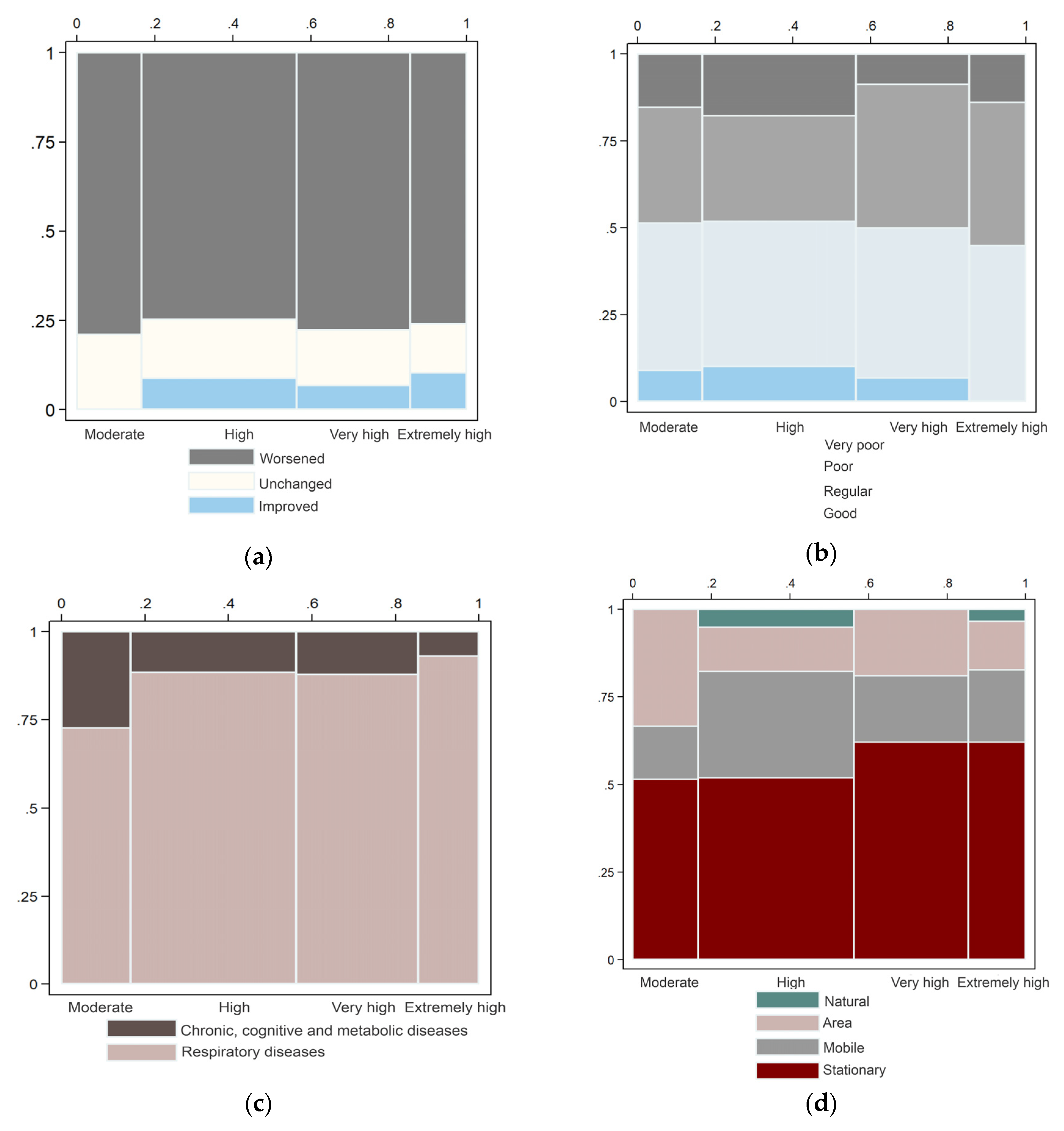
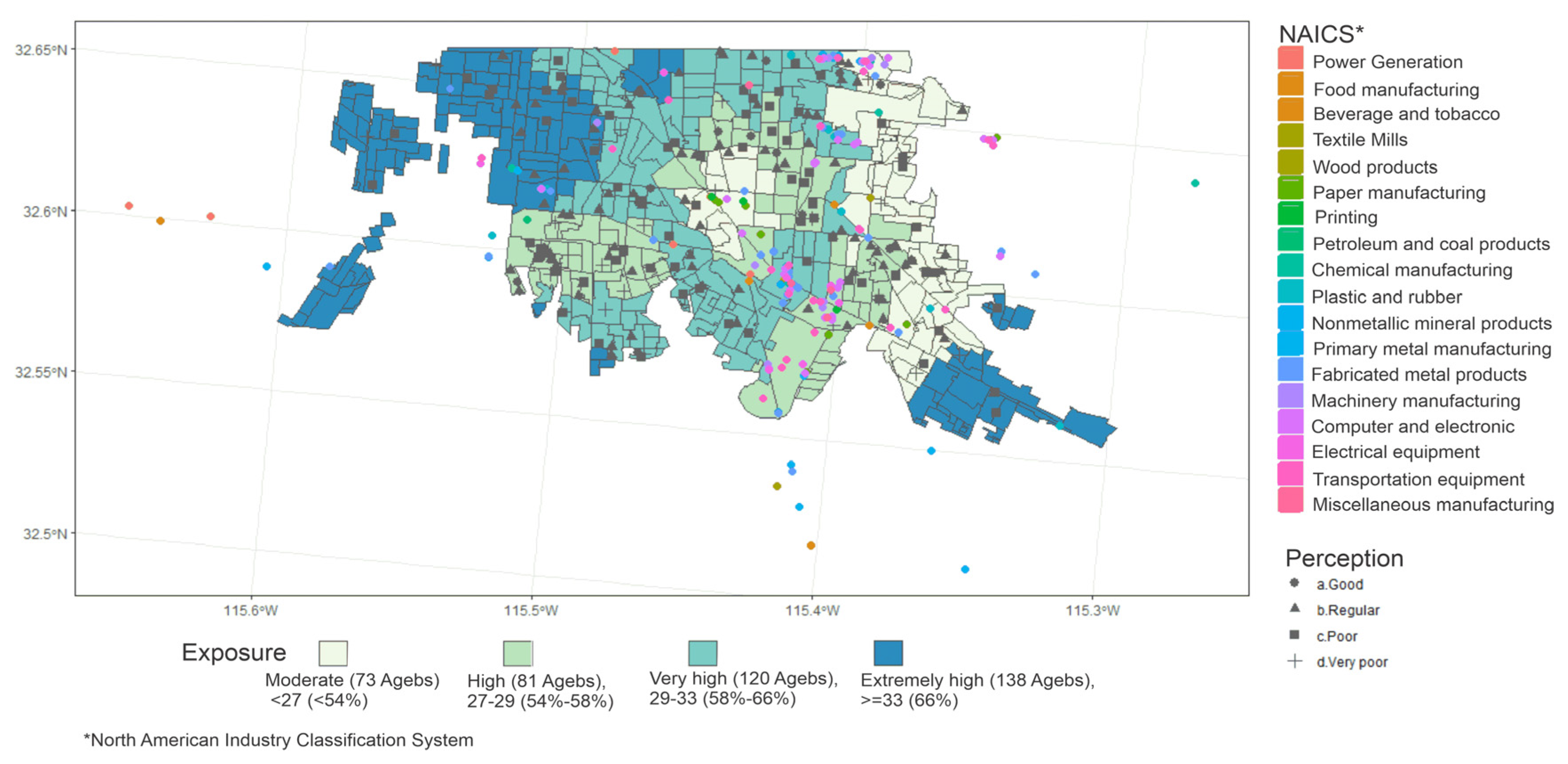
3.4.2. Spatial Distribution of Air Quality Perception, Estimated Exposure to PM10 and Stationary Sources of Pollution
3.5. Statistical Model for the Association between Perceived Air Quality, Socioeconomic Attributes, and Estimated Exposure to PM10
4. Discussion
4.1. Linking Air Pollution and Social Vulnerability
4.2. The Association of Air Pollution, Socioeconomic Attributes and Air Quality Perception
4.3. Limitations
5. Conclusions
Supplementary Materials
Author Contributions
Funding
Acknowledgments
Conflicts of Interest
References
- Organization for Economic Co-operation and Development OECD. The Economic Consequences of Outdoor Air Pollution; Organization for Economic Co-operation and Development OECD: Paris, France, 2016. [Google Scholar] [CrossRef]
- World Health Organization. Ambient Air Pollution: A Global Assessment of Exposure and Burden of Disease. Available online: https://www.who.int/phe/publications/air-pollution-global-assessment/en/ (accessed on 10 June 2020).
- World Health Organization. Fact Sheets. Detail. Ambient (Outdoor) Air Quality and Health. 2014. Available online: https://www.who.int/en/news-room/fact-sheets/detail/ambient-(outdoor)-air-quality-and-health (accessed on 1 October 2019).
- World Health Organization. Global Ambient Air Quality Database (Update 2018). Available online: https://www.who.int/airpollution/data/en/ (accessed on 3 January 2020).
- Organization & UN-Habitat 2016. Global Report on Urban Health: Equitable Healthier Cities for Sustainable Development. Available online: https://apps.who.int/iris/handle/10665/204715 (accessed on 3 January 2020).
- Haines, A.; Amann, M.; Borgford-Parnell, N.; Leonard, S.; Kuylenstierna, J.; Shindell, D. Short-lived climate pollutant mitigation and the Sustainable Development Goals. Nat. Clim. Chang. 2017, 7, 863–869. [Google Scholar] [CrossRef]
- Ezzati, M.; Utzinger, J.; Cairncross, S.; Cohen, A.J.; Singer, B.H. Environmental risks in the developing world: Exposure indicators for evaluating intervention, programmes, and policies. J. Epidemiol. Commun. Health 2005, 59, 15–22. [Google Scholar] [CrossRef]
- Majid, H.M.; Madl, P.; Alam, K. Ambient air quality with emphasis on roadside junctions in metropolitan cities of Pakistan and its potential health effects. Health 2012, 3, 79–85. [Google Scholar]
- Mannucci, P.M.; Franchini, M. Health effects of ambient air pollution in developing countries. Int. J. Environ. Res. Public Health 2017, 14, 1048. [Google Scholar] [CrossRef]
- Martins, N.R.; Carrilho da Graça, G. Impact of PM2.5 in indoor urban environments: A review. Sustain. Cities Soc. 2018, 42, 259–275. [Google Scholar] [CrossRef]
- Romieu, I.; Gouveia, N.; Cifuentes, L.A.; de Leon, A.P.; Junger, W.; Vera, J.; Strappa, V.; Hurtado-Díaz, M.; Miranda-Soberanis, V.; Rojas-Bracho, L. Multicity study of air pollution and mortality in Latin America (the ESCALA study). Resp. Rep. Health Eff. Inst. 2012, 171, 5–86. [Google Scholar]
- Díaz-Robles, L.A.; Fu, J.S.; Vergara-Fernández, A.; Etcharren, P.; Schiappacasse, L.N.; Reed, G.D.; Silva, M.P. Health risks caused by short term exposure to ultrafine particles generated by residential wood combustion: A case study of Temuco, Chile. Environ. Int. 2014, 66, 174–181. [Google Scholar] [CrossRef] [PubMed]
- Arceo, E.; Hanna, R.; Oliva, P. Does the effect of pollution on infant mortality differ between developing and developed countries? Evidence from Mexico City. Econ. J. 2015, 126, 257–280. [Google Scholar] [CrossRef]
- Landrigan, P.J.; Fuller, R. Pollution, health and development: The need for a new paradigm. Rev. Environ. Health 2016, 31, 121–124. [Google Scholar] [CrossRef] [PubMed]
- Martenies, S.E.; Milando, C.W.; Williams, G.O.; Batterman, S.A. Disease and Health Inequalities Attributable to Air Pollutant Exposure in Detroit, Michigan. Int. J. Environ. Res. Public Health 2017, 14, 1243. [Google Scholar] [CrossRef]
- Caplin, A.; Ghandehari, M.; Lim, C.; Glimcher, P.; Thurston, G. Advancing environmental exposure assessment science to benefit society. Nat. Commun. 2019, 10, 1236. [Google Scholar] [CrossRef] [PubMed]
- Lome-Hurtado, A.; Touza-Montero, J.; White, P.C.L. Environmental Injustice in Mexico City: A Spatial Quantile Approach. Expo. Health 2020, 12, 265–279. [Google Scholar] [CrossRef]
- Benmarhnia, T.; Rey, L.; Cartier, Y.; Christelle, M.C.; Deguen, S.; Brousselle, A. Addressing equity in interventions to reduce air pollution in urban areas: A systematic review. Int. J. Public Health 2014, 59, 933–944. [Google Scholar] [CrossRef] [PubMed]
- Armaş, I. Social vulnerability and seismic risk perception. Case study: The historic center of the Bucharest Municipality/Romania. Nat. Hazards 2008, 47, 387–410. [Google Scholar] [CrossRef]
- Cutter, S.L.; Boruff, B.J.; Shirley, W.L. Social Vulnerability to Environmental Hazards. Soc. Sci. Q. 2003, 84, 241–261. [Google Scholar] [CrossRef]
- Ge, Y.; Zhang, H.; Dou, W.; Chen, W.; Liu, N.; Wang, Y.; Shi, Y.; Rao, W. Mapping Social Vulnerability to Air Pollution: A Case Study of the Yangtze River Delta Region, China. Sustainability 2017, 9, 109. [Google Scholar] [CrossRef]
- Nilsson, M.; Griggs, D.; Visbeck, M. Policy: Map the interactions between Sustainable Development Goals. Nature 2016, 534, 320–322. [Google Scholar] [CrossRef]
- Longhurst, J.; Barnes, J.; Chatterton, T.; De Vito, L.; Everard, M.; Hayes, E.P.; Williams, B. Analysing air pollution and its management through the lens of the un sustainable development goals: A review and assessment. WIT Trans. Ecol. Environ. 2018, 230, 3–14. [Google Scholar] [CrossRef]
- Pu, S.; Shao, Z.; Fang, M.; Yang, L.; Liu, R.; Bi, J.; Ma, Z. Spatial distribution of the public’s risk perception for air pollution: A nationwide study in China. Sci. Total Environ. 2019, 655, 454–462. [Google Scholar] [CrossRef]
- Bickerstaff, K.; Walker, G. Clearing the smog? Public responses to air-quality information. Local Environ. 1999, 4, 279–294. [Google Scholar] [CrossRef]
- Bickerstaff, K. Risk perception research: Socio-cultural perspectives on the public experience of air pollution. Environ. Int. 2004, 30, 827–840. [Google Scholar] [CrossRef] [PubMed]
- Bickerstaff, K.; Walker, G. Public understandings of air pollution: The ‘localisation’ of environmental risk. Glob. Environ. Chang. 2001, 11, 133–145. [Google Scholar] [CrossRef]
- Oltra, C.; Sala, R. Perception of risk from air pollution and reported behaviors: A cross-sectional survey study in four cities. J. Risk Res. 2018, 21, 869–884. [Google Scholar] [CrossRef]
- Kim, M.; Yi, O.; Kim, H. The role of differences in individual and community attributes in perceived air quality. Sci. Total Environ. 2012, 425, 20–26. [Google Scholar] [CrossRef]
- Liu, X.; Zhu, H.; Hu, Y.; Feng, S.; Chu, Y.; Wu, Y.; Wang, C.; Zhan, Y.; Yuan, Z.; Lu, Y. Public’s Health Risk Awareness on Urban Air Pollution in Chinese Megacities: The Cases of Shanghai, Wuhan and Nanchang. Int. J. Environ. Res. 2016, 13, 845. [Google Scholar] [CrossRef]
- Boso, À.; Álvarez, B.; Oltra, C.; Hofflinger, A.; Vallejos-Romero, A.; Garrido, J. Examining Patterns of Air Quality Perception: A Cluster Analysis for Southern Chilean Cities. SAGE Open 2019, 9, 1–11. [Google Scholar] [CrossRef]
- Ramírez, O.; Mura, I.; Franco, J.F. How Do People Understand Urban Air Pollution? Exploring Citizens’ Perception on Air Quality, Its Causes and Impacts in Colombian Cities. Open J. Air Pollut. 2017, 6, 1–17. [Google Scholar] [CrossRef]
- Catalán-Vázquez, M.; Riojas-Rodríguez, H.; Jarillo-Soto, E.C.; Delgadillo-Gutiérrez, H.J. Percepción de riesgo a la salud por contaminación del aire en adolescentes de la Ciudad de México. Salud Publica Mex. 2009, 51, 148–156. [Google Scholar] [CrossRef][Green Version]
- Peng, M.; Zhang, H.; Evans, R.D.; Zhong, X.; Yang, K. Actual Air Pollution, Environmental Transparency, and the Perception of Air Pollution in China. J. Environ. Dev. 2009, 28, 78–105. [Google Scholar] [CrossRef]
- Infante, C.; Idrovo, A.J.; Sánchez-Domínguez, M.S.; Vinhas, S.; González-Vázquez, T. Violence committed against migrants in transit: Experiences on the Northern Mexican Border. J. Immigr. Minor Health 2011, 14, 449–459. [Google Scholar] [CrossRef]
- Carruthers, D. Environmental Justice in Latin America: Problems, Promise and Practice; Carruthers, D., Ed.; MIT Press: Cambridge, MA, USA, 2008; pp. 136–160. [Google Scholar]
- Meza, L.M.; Quintero, M.; García, R.; Ramírez, J. Estimación de Factores de Emisión de PM10 y PM2.5, en vías urbanas en Mexicali, Baja California, México. Información Tecnológica 2010, 21, 45–56. [Google Scholar] [CrossRef]
- Osornio-Vargas, A.R.; Serrano, J.; Rojas-Bracho, L.; Miranda, J.; Garcia-Cuellar, C.; Reyna, M.A.; Sánchez-Pérez, Y. In vitro biological effects of airborne PM2.5 and PM10 from a semi-desert city on the Mexico-US border. Chemosphere 2011, 83, 618–626. [Google Scholar] [CrossRef] [PubMed]
- Wilder, M.; Scott, C.A.; Pineda, N.P.; Varady, R.G.; Garfin, G.M.; McEvoy, J. Adapting Across Boundaries: Climate Change, Social Learning, and Resilience in the U.S.- Mexico Border Region. Ann. Am. Assoc. Geogr. 2010, 100, 917–928. [Google Scholar] [CrossRef]
- Lusk, M.; Staudt, K.; Moya, E.M. Social Justice in the US-Mexico Border Region, 1st ed.; Springer: New York, NY, USA, 2012; pp. 3–38. ISBN 978-94-007-4150-8. [Google Scholar]
- Heyman, J. Environmental issues at the US-Mexico border and the unequal territorialization of value. In Rethinking Environmental History: World-Systems History and Global Environmental Change; Hornberg, A.J., McNeill, J.R., Martinez-Alier, J., Eds.; Altamira Press: Lanham, UK, 2007; pp. 327–343. [Google Scholar]
- Mollick, A.V.; Cortez-Rayas, A.; Olivas-Moncisvais, R.A. Local labor markets in U.S.–Mexican border cities and the impact of maquiladora production. Ann. Reg. Sci. 2006, 40, 95–116. [Google Scholar] [CrossRef]
- Norman, L.M.; Villareal, M.L.; Lara-Valencia, F.; Yuan, Y.; Nie, W.; Wilson, S.; Amaya, G.; Sleeter, R. Mapping socio-environmentally vulnerable populations access and exposure to ecosystem services at the U.S.–Mexico borderlands. Appl. Geogr. 2012, 34, 413–424. [Google Scholar] [CrossRef]
- INEGI. Censo de Población y Vivienda, Instituto Nacional de Estadística y Geografía, México. 2010. Available online: Inegi.org.mx/programas/ccpv/2010/ (accessed on 5 April 2020).
- García, O.R.; Jáuregui, E.; Toudert, D.; Tejeda, A. Detection of the urban heat island in Mexicali, B.C., Mexico and its relationship with land use. Atmósfera 2007, 20, 111–131. [Google Scholar]
- Rojas-Caldelas, R.; Peña-Salmon, C.; Corona-Zambrano, E.; Arias-Vallejo, A.; Leyva-Camacho, O. Environmental Sustainability Agenda: Metropolitan Area of Mexicali, Baja California, Mexico. WIT Trans. Ecol. Environ. 2013, 173, 267–277. [Google Scholar] [CrossRef]
- INECC. Informe Nacional de Calidad del Aire 2017, México. Coordinación General de Contaminación y Salud Ambiental, Dirección de Investigación de Calidad del Aire y Contaminantes Climáticos; Instituto Nacional de Ecología y Cambio Climático: Ciudad de México, Mexico, 2018; Available online: https://www.gob.mx/inecc/prensa/inecc-pone-a-disposicion-el-informe-nacional-de-calidad-del-aire-2017?idiom=es (accessed on 5 April 2020).
- Quintero-Nuñez, M.; Sweedler, A. Air quality evaluation in the Mexicali and Imperial Valleys as an element for an Outreach Program. In Imperial-Mexicali Valleys: Development and Environment of the U.S.-Mexican Border Region; Collins, K., Ed.; Institute for Regional Studies of the Californias and SDSU Press: San Diego, CA, USA, 2004; pp. 263–280. [Google Scholar]
- SEMARNAT & EPA. Programa Ambiental México-Estados Unidos: Frontera. 2020. Available online: https://www.gob.mx/semarnat/acciones-y-programas/publicaciones-del-programa (accessed on 5 April 2020).
- Canales-Rodríguez, M.; Quintero-Nuñez, M.; Castro-Romero, T.G.; García-Cueto, R.O. Las partículas respirables PM10 y su composición química en la zona urbana y rural de Mexicali, Baja California en México. Información Tecnológica 2014, 25, 13–22. [Google Scholar] [CrossRef]
- Eades, L. Air pollution at the US-Mexico border: Strengthening the framework for bilateral cooperation. J. Public Int. Aff. 2018, 29, 64–78. [Google Scholar]
- Jerrett, M.; Gale, S.; Kontgis, C. Spatial Modeling in Environmental and Public Health Research. Int. J. Environ. Res. Public Health 2010, 7, 1302–1329. [Google Scholar] [CrossRef]
- Téllez-Rojo, M.M.; Rothenberg, S.J.; Texcalac-Sangrador, J.L.; Just, A.C.; Kloog, I.; Rojas-Saunero, L.P.; Gutiérrez-Avila, I.; Bautista-Arredondo, L.F.; Tamayo-Ortiz, M.; Romero, M. Children’s acute respiratory symptoms associated with PM2.5 estimates in two sequential representative surveys from the Mexico City Metropolitan Area. Environ. Res. 2020, 180, 108868. [Google Scholar] [CrossRef] [PubMed]
- Evans, G.W.; Kantrowitz, E. Socioeconomic status and health: The potential role of environmental risk exposure. Annu. Rev. Public Health 2002, 23, 303–331. [Google Scholar] [CrossRef] [PubMed]
- Ho, H.C.; Wong, M.S.; Yang, L.; Chan, T.C.; Bilal, M. Influences of socioeconomic vulnerability and intra-urban air pollution exposure on short-term mortality during extreme dust events. Environ. Pollut 2018, 155–162. [Google Scholar] [CrossRef] [PubMed]
- Cortinovis, I.; Vela, V.; Ndiku, J. Construction of a socio-economic index to facilitate analysis of health in data in developing countries. Soc. Sci. Med. 1993, 36, 1087–1097. [Google Scholar] [CrossRef]
- Cattell, R.B. The scree test for the number of factors. Multivar. Behav. Res. 1996, 1, 245–276. [Google Scholar] [CrossRef]
- Anselin, L. Spatial effects in econometric practice in environmental and resource economics. Am. J. Agr. Econ. 2001, 83, 705–710. [Google Scholar] [CrossRef]
- Anselin, L.; Syabri, I.; Kho, Y. GeoDa: An Introduction to Spatial Data Analysis. Geogr. Anal. 2006, 38, 5–22. [Google Scholar] [CrossRef]
- Muñoz-Pizza, D.M.; Villada-Canela, M.; Rivera-Castañeda, P.; Reyna-Carranza, M.A.; Osornio-Vargas, A.; Martínez-Cruz, A.L. Stated benefits from improved air quality through urban afforestation in an arid city: A contingent valuation in Mexicali, Baja California, Mexico. Urban For. Urban Green 2020. (under review). [Google Scholar]
- INEGI. Directorio Estadístico Nacional de Unidades Económicas (DENUE). Actividades Económicas Industrials. 2019. Available online: https://www.inegi.org.mx/app/descarga/?ti=6 (accessed on 5 April 2020).
- Zandbergern, A.; Chakaraborty, J. Improving environmental exposure analysis using cumulative distribution functions and individual geocoding. Int. J. Health Geogr. 2006, 5, 23. [Google Scholar] [CrossRef] [PubMed]
- Chakraborty, J.; Maantay, J.A. Proximity Analysis for exposure assessment in environmental health justice research. In Geospatial Analysis of Environmental Health; Maantay, J., McLafferty, S., Eds.; Geotechnologies and the Environment Series; Springer: Dordrecht, The Netherlands, 2011; pp. 111–138. [Google Scholar]
- Brody, S.D.; Peck, B.M.; Highfield, W.E. Examining Localized Patterns of Air Quality Perception in Texas: A Spatial and Statistical Analysis. Risk Anal. 2004, 24, 1561–1574. [Google Scholar] [CrossRef]
- Huang, L.; Rao, C.; van der Kuijp, T.J.; Bi, J.; Liu, Y. A comparison of individual exposure, perception, and acceptable levels of PM2.5 with air pollution policy objectives in China. Environ. Res. 2017, 157, 78–86. [Google Scholar] [CrossRef]
- Schmitz, S.; Weiand, L.; Becker, S.; Niehoff, N.; Schwartzbach, F.; von Schneidemesser, E. An assessment of perceptions of air quality surrounding the implementation of a traffic-reduction measure in a local urban environment. Sustain. Cities Soc. 2018, 41, 525–537. [Google Scholar] [CrossRef]
- Reames, T.G.; Bravo, M.A. People, place and pollution. Investigating relationships between air quality perceptions, health concerns, exposure, and individual-and-are-level characteristics. Environ. Int. 2019, 122, 244–255. [Google Scholar] [CrossRef] [PubMed]
- Vargha, A.; Delaney, H.D. The Kruskal-Wallis Test and Stochastic Homogeneity. J. Edu. Behav. Stat. 1998, 23, 170–192. [Google Scholar] [CrossRef]
- Wolfe, R.; Gould, W. An Approximate Likelihood-Ratio Test for Ordinal Response Models; Stata Technical Bulletin; StataCorp Lp: College Station, TX, USA, 1998; Volume 7, pp. 24–27. Available online: http://stata-press.com/journals/stbcontents/stb42.pdf (accessed on 5 April 2020).
- Hill, R.C.; Griffiths, W.E.; Lim, G.C. Qualitative and Limited Dependent Variable Models. In Principles of Econometrics, 5th ed.; John Wiley & Sons: New York, NY, USA, 2018; pp. 702–718. [Google Scholar]
- Encuesta Nacional de Ingresos y Gastos de los Hogares ENIGH 2019. Instituto Nacional de Estadística y Geografía, México. Available online: https://www.inegi.org.mx/programas/enigh/nc/2018/ (accessed on 5 April 2020).
- World Development Indicators, The World Bank Databank. 2019. Available online: https://databank.worldbank.org/reports.aspx?source=2&series=PA.NUS.FCRF&country= (accessed on 15 January 2020).
- Corona Zambrano, E.A.; Rojas-Caldelas, R.I. Environmental Planning and Management of Air Quality: The Case of Mexicali, Baja California, Mexico. WIT Trans. Ecol. Environ. 2008, 116, 419–427. [Google Scholar] [CrossRef]
- Aguilar-Dodier, L.C.; Castillo, J.E.; Quintana, J.E.P.; Montoya, L.D.; Molina, L.T.; Zavala, M.; Almanza-Veloz, V.; Rodríguez-Ventura, J.G. Spatial and temporal evaluation of H2S, SO2 and NH3 concentrations near Cerro Prieto geothermal power plant in Mexico. Atmos. Pollut. Res. 2020, 11, 94–104. [Google Scholar] [CrossRef]
- Grineski, S.E.; Collins, T.W. Exploring patterns of environmental injustice in the Global South: Maquiladoras in Ciudad Juárez, Mexico. Popul. Environ. 2008, 29, 247–270. [Google Scholar] [CrossRef]
- Grineski, S.E.; Juárez-Carillo, P.M. Social Justice in the U.S.–Mexico Border Region; Lusk, M., Staudt, K., Moya, E., Eds.; Springer: Dordrecht, The Netherlands, 2012; pp. 179–198. [Google Scholar]
- Agenda 2030, Estrategia Nacional para la Implementación de la Agenda 2030 en México. 2019. Available online: https://www.gob.mx/agenda2030/documentos/estrategia-nacional-de-la-implementacion-de-la-agenda-2030-para-el-desarrollo-sostenible-en-mexico?idiom=es (accessed on 5 April 2020).
- Hao, Y.; Liu, Y.M. The influential factors of urban PM2.5 concentrations in China: A spatial econometric analysis. J. Clean. Prod. 2016, 112, 1443–1453. [Google Scholar] [CrossRef]
- Dong, D.; Xu, X.; Xu, W.; Xie, J. The Relationship Between the Actual Level of Air Pollution and Residents’ Concern about Air Pollution: Evidence from Shanghai, China. Int. J. Environ. Res. Public Health 2019, 16, 4784. [Google Scholar] [CrossRef]
- Imran, M.; Sumra, K.; Abbas, N.; Majeed, I. Spatial distribution and opportunity mapping: Applicability of evidence-based policy implications in Punjab using remote sensing and global products. Sustain. Cities Soc. 2019, 50, 101652. [Google Scholar] [CrossRef]
- Elliott, S.J.; Cole, D.C.; Krueger, P.; Voorberg, N.; Wakefield, S. The power of perception: Health risk attributed to air pollution in an urban industrial neighborhood. Risk Anal. 1999, 19, 621–634. [Google Scholar] [CrossRef] [PubMed]
- Ley-García, J.; Denegri de Dios, F.M.; Ortega-Villa, L.M. Spatial dimension of urban hazardscape perception: The case of Mexicali, Mexico. Int. J. Disaster Risk Reduct. 2015, 14, 487–495. [Google Scholar] [CrossRef]
- Calvillo, N.; Garnett, E. Data intimacies: Building infrastructures for intensified embodied encounters with air pollution. Sociol. Rev. 2019, 67, 340–356. [Google Scholar] [CrossRef]
- Yang, J.; Zou, L.; Lin, T.; Wu, Y.; Wang, H. Public willingness to pay for CO2 mitigation and the determinants under climate change: A case study of Suzhou, China. J. Environ. Manag. 2014, 146, 1–8. [Google Scholar] [CrossRef]


| Variables 1 | N | Mean | Std. Dev. | Min | Max |
|---|---|---|---|---|---|
| Population without post-basic education 2 | 370 | 687.43 | 540.49 | 1 | 4290 |
| Population without employment 3 | 357 | 42.11 | 30.69 | 0 | 168 |
| Population without health insurance (public/private) | 370 | 458.70 | 301.12 | 0 | 1503 |
| Number of households headed by women | 370 | 149.54 | 100.19 | 0 | 470 |
| Number of people per room (overcrowding proxy) | 370 | 3.43 | 0.51 | 2 | 4 |
| Household without a car | 370 | 136.46 | 115.07 | 0 | 750 |
| Variable | Description | Odds Ratio | 95% CI |
|---|---|---|---|
| Average monthly household income (2019 USD) 1 | <US $354.9 (Ref) | ||
| From US $354.9 to US $605.4 | 0.36 ** | [0.15–0.90] | |
| From US $605.4 to US $1352 | 0.30 ** | [0.11–0.86] | |
| From US $1352 to US $1825 | 0.42 | [0.08–2.20] | |
| >US $1825 | 0.48 | [0.11–2.02] | |
| Knowledge of health effects related to air pollution 2 | No (Ref) | ||
| Yes | 0.51 | [0.13–1.96] | |
| Perception of air quality in the location of the individual’s residence 3 | Good (Ref) | ||
| Regular | 0.41 | [0.14–1.21] | |
| Poor | 0.21 *** | [0.07–0.69] | |
| Very poor | 0.32 * | [0.08–1.21] | |
| Exposure areas by exceedance days of PM10 concentrations 4 | Moderate (Ref) | ||
| High | 1.22 | [0.44–3.39] | |
| Very high | 1.27 | [0.43–3.78] | |
| Extremely high | 1.58 | [0.42–5.91] | |
| Social vulnerability (categories by SES index) 5 | Medium-high SES index (Ref) | ||
| Low SES index | 0.58 | [0.24–1.38] | |
| N = 199 Log-likelihood = −127.54 | |||
| Equality coefficient test through the response Chi2(12) = 2.37 Categories 6 Pseudo R2 = 0.78 | |||
© 2020 by the authors. Licensee MDPI, Basel, Switzerland. This article is an open access article distributed under the terms and conditions of the Creative Commons Attribution (CC BY) license (http://creativecommons.org/licenses/by/4.0/).
Share and Cite
Muñoz-Pizza, D.M.; Villada-Canela, M.; Reyna, M.A.; Texcalac-Sangrador, J.L.; Serrano-Lomelin, J.; Osornio-Vargas, Á. Assessing the Influence of Socioeconomic Status and Air Pollution Levels on the Public Perception of Local Air Quality in a Mexico-US Border City. Int. J. Environ. Res. Public Health 2020, 17, 4616. https://doi.org/10.3390/ijerph17134616
Muñoz-Pizza DM, Villada-Canela M, Reyna MA, Texcalac-Sangrador JL, Serrano-Lomelin J, Osornio-Vargas Á. Assessing the Influence of Socioeconomic Status and Air Pollution Levels on the Public Perception of Local Air Quality in a Mexico-US Border City. International Journal of Environmental Research and Public Health. 2020; 17(13):4616. https://doi.org/10.3390/ijerph17134616
Chicago/Turabian StyleMuñoz-Pizza, Dalia M., Mariana Villada-Canela, M. A. Reyna, José Luis Texcalac-Sangrador, Jesús Serrano-Lomelin, and Álvaro Osornio-Vargas. 2020. "Assessing the Influence of Socioeconomic Status and Air Pollution Levels on the Public Perception of Local Air Quality in a Mexico-US Border City" International Journal of Environmental Research and Public Health 17, no. 13: 4616. https://doi.org/10.3390/ijerph17134616
APA StyleMuñoz-Pizza, D. M., Villada-Canela, M., Reyna, M. A., Texcalac-Sangrador, J. L., Serrano-Lomelin, J., & Osornio-Vargas, Á. (2020). Assessing the Influence of Socioeconomic Status and Air Pollution Levels on the Public Perception of Local Air Quality in a Mexico-US Border City. International Journal of Environmental Research and Public Health, 17(13), 4616. https://doi.org/10.3390/ijerph17134616