Prioritizing and Analyzing the Role of Climate and Urban Parameters in the Confirmed Cases of COVID-19 Based on Artificial Intelligence Applications

 ,
,  ,
,  ,
, 

 and
and 
Abstract
1. Introduction
2. Methodology
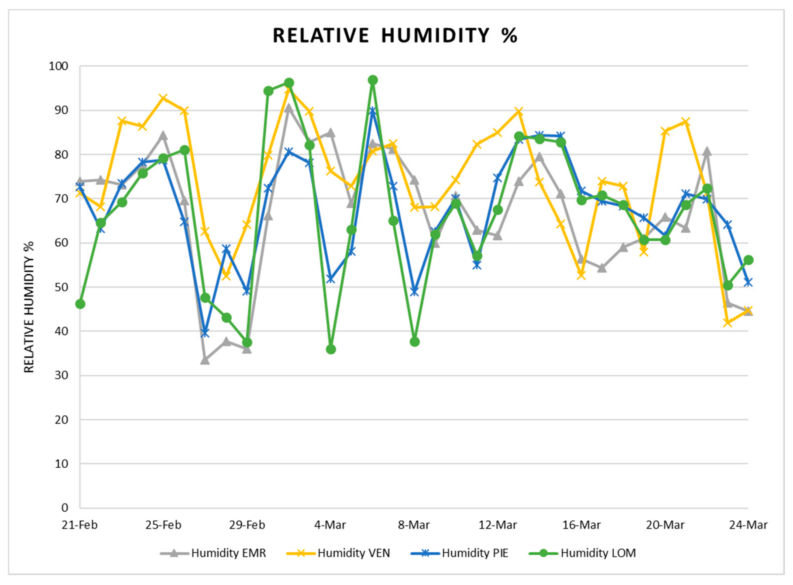
- The analysis factors are the population density of each region, average daily temperature, relative humidity, wind speed, and the positive cases in the following days;
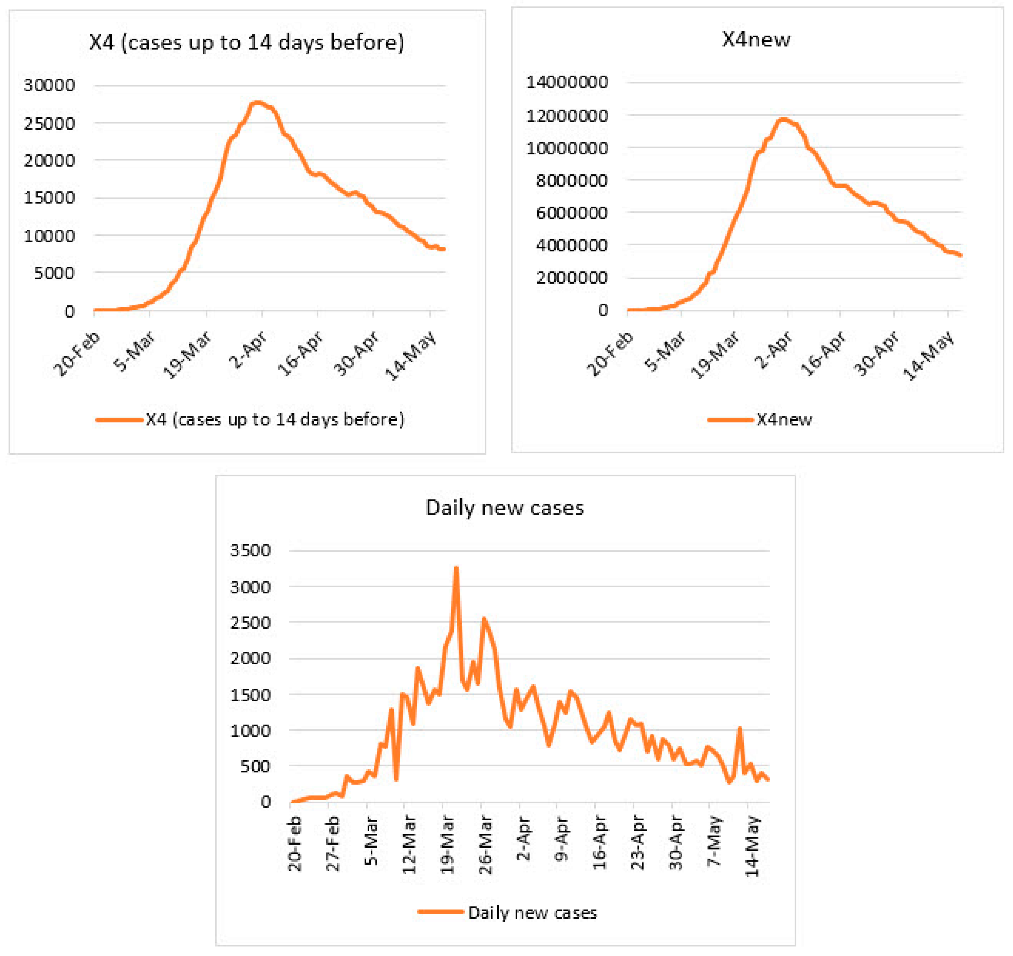
- Since the incubation period of the virus is about 14 days, the sum of previous positive cases up to 14 days previously has been considered;
- The analysis period is from 14 February 2020 to 24 March 2020.
2.1. Artificial Intelligence Methods
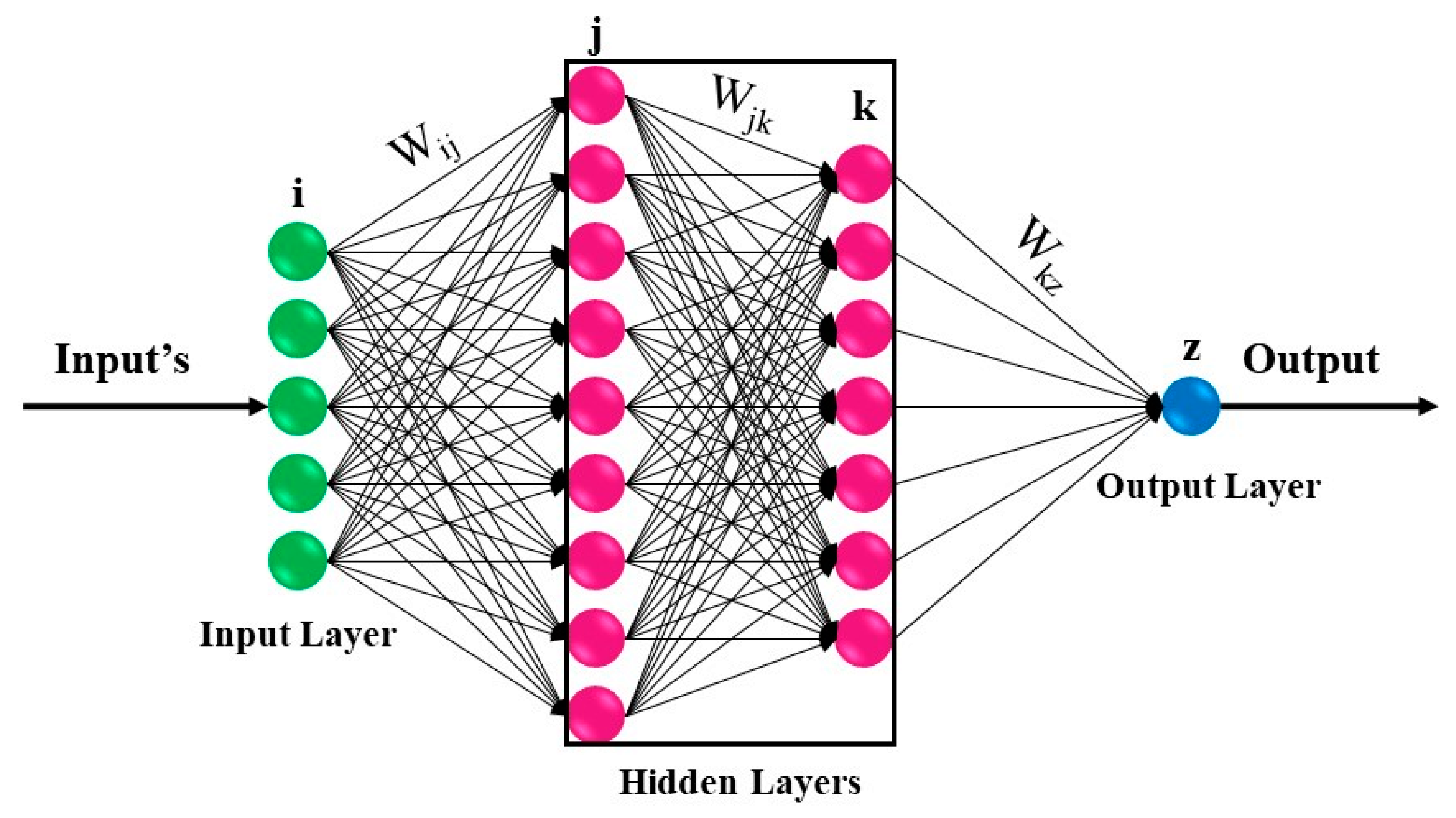
2.1.1. Artificial Neural Network (ANN)
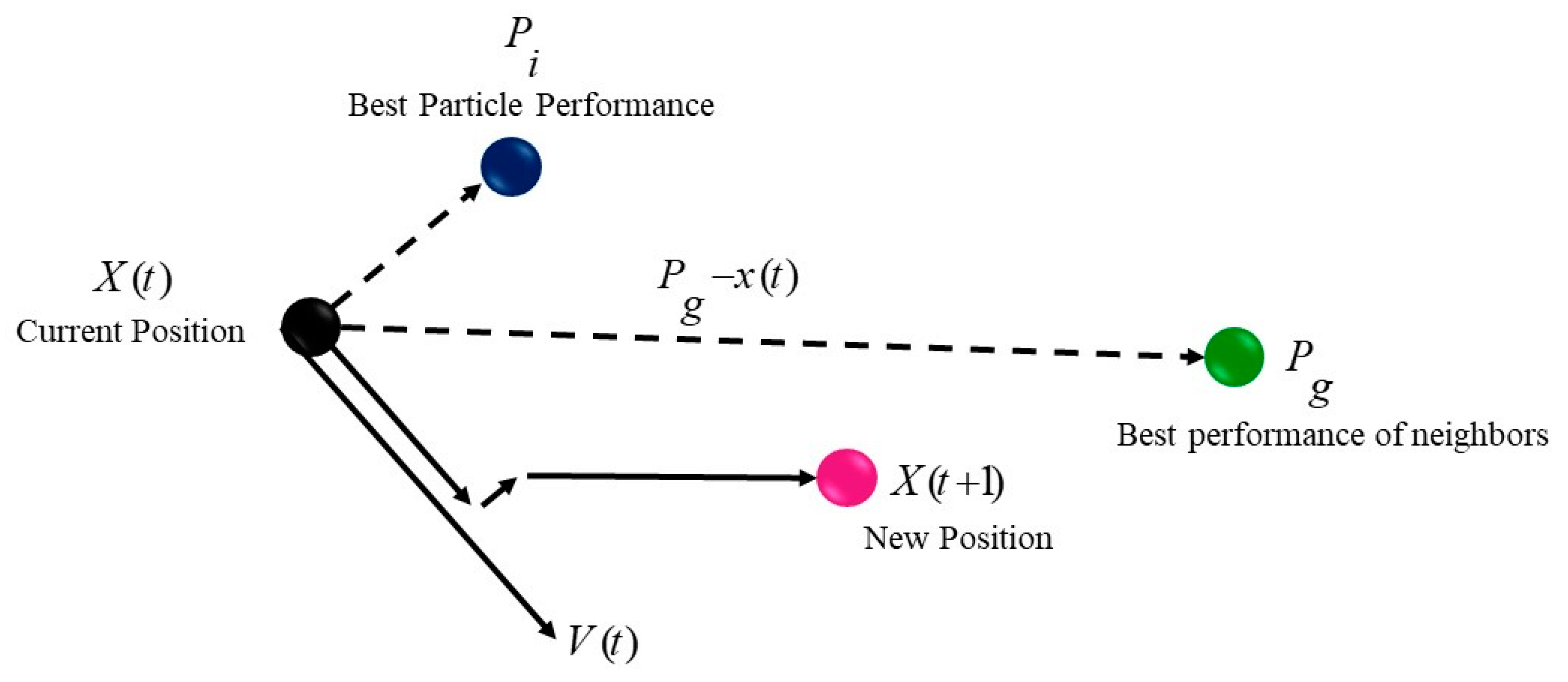
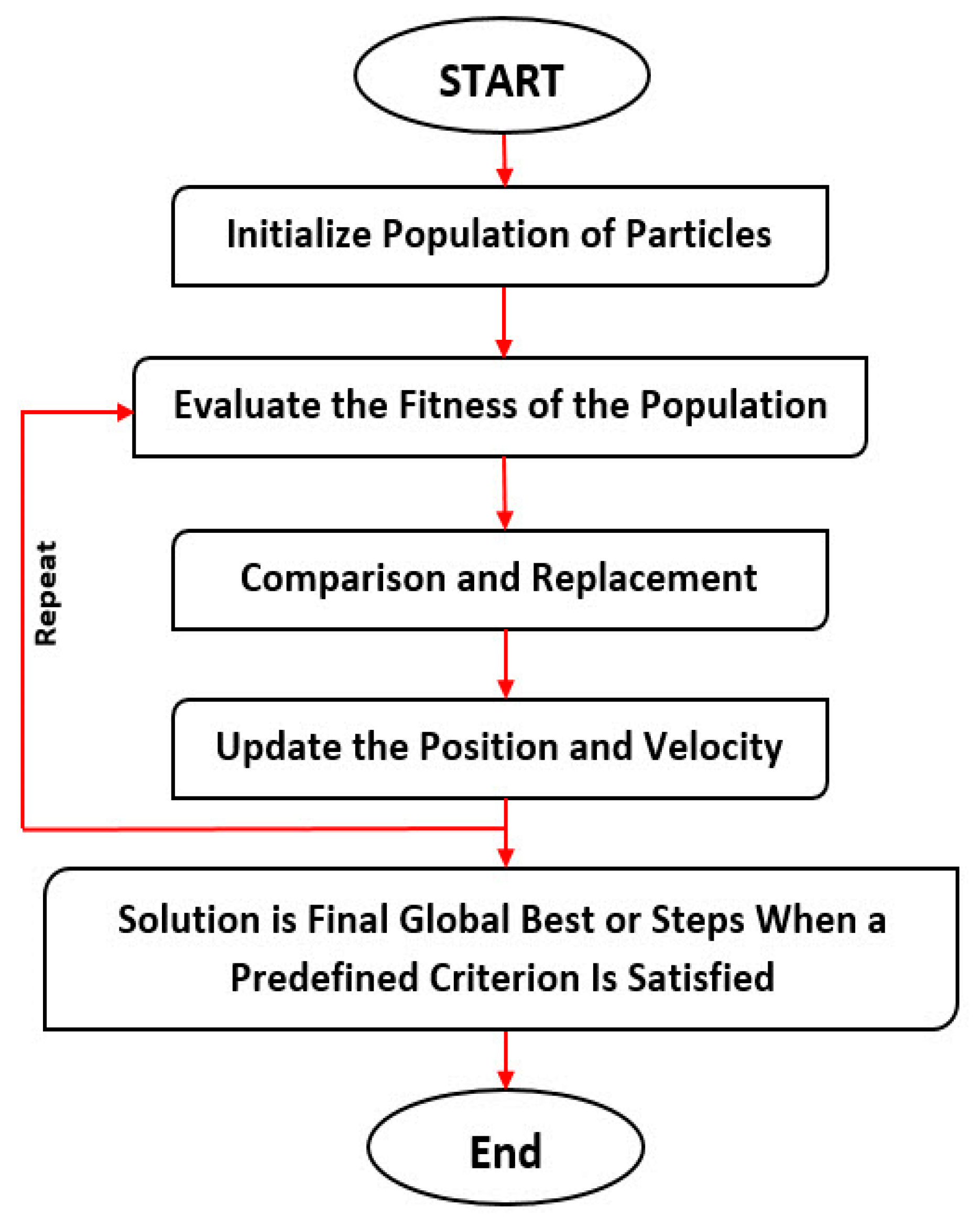
2.1.2. Particle Swarm Optimization (PSO) Algorithm
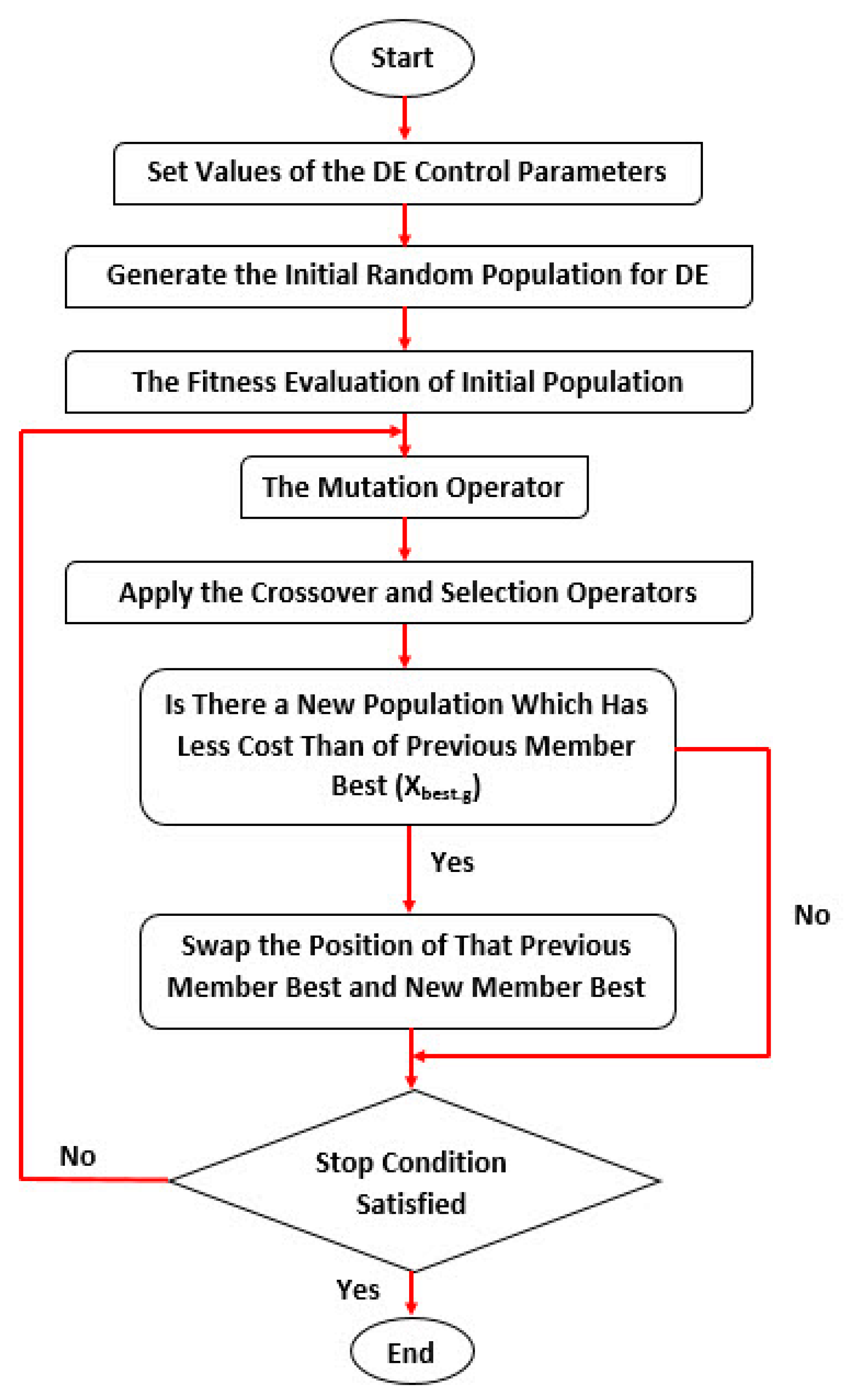
2.1.3. Differential Evolution (DE) Algorithm
2.2. Subsection
3. Model Development
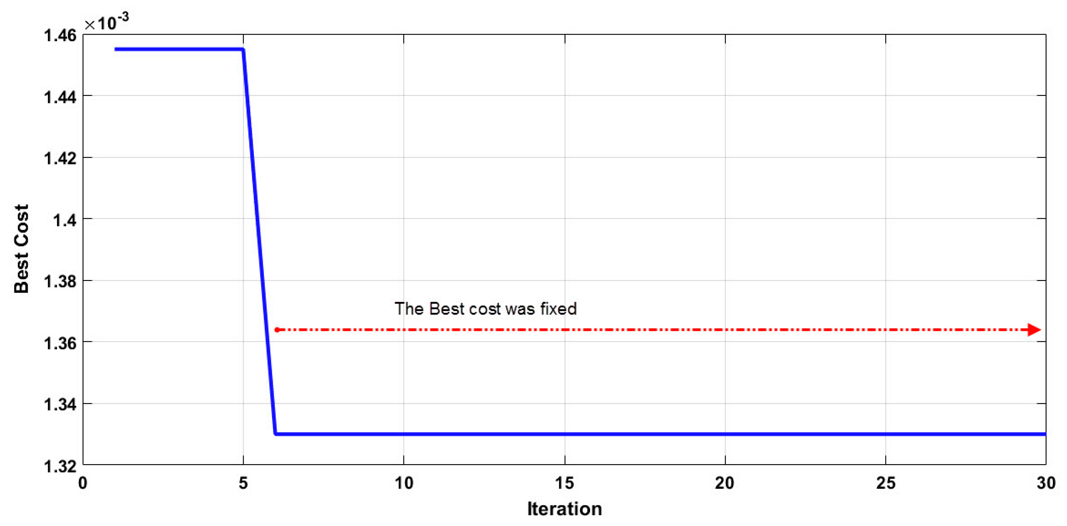
3.1. PSO Modelling
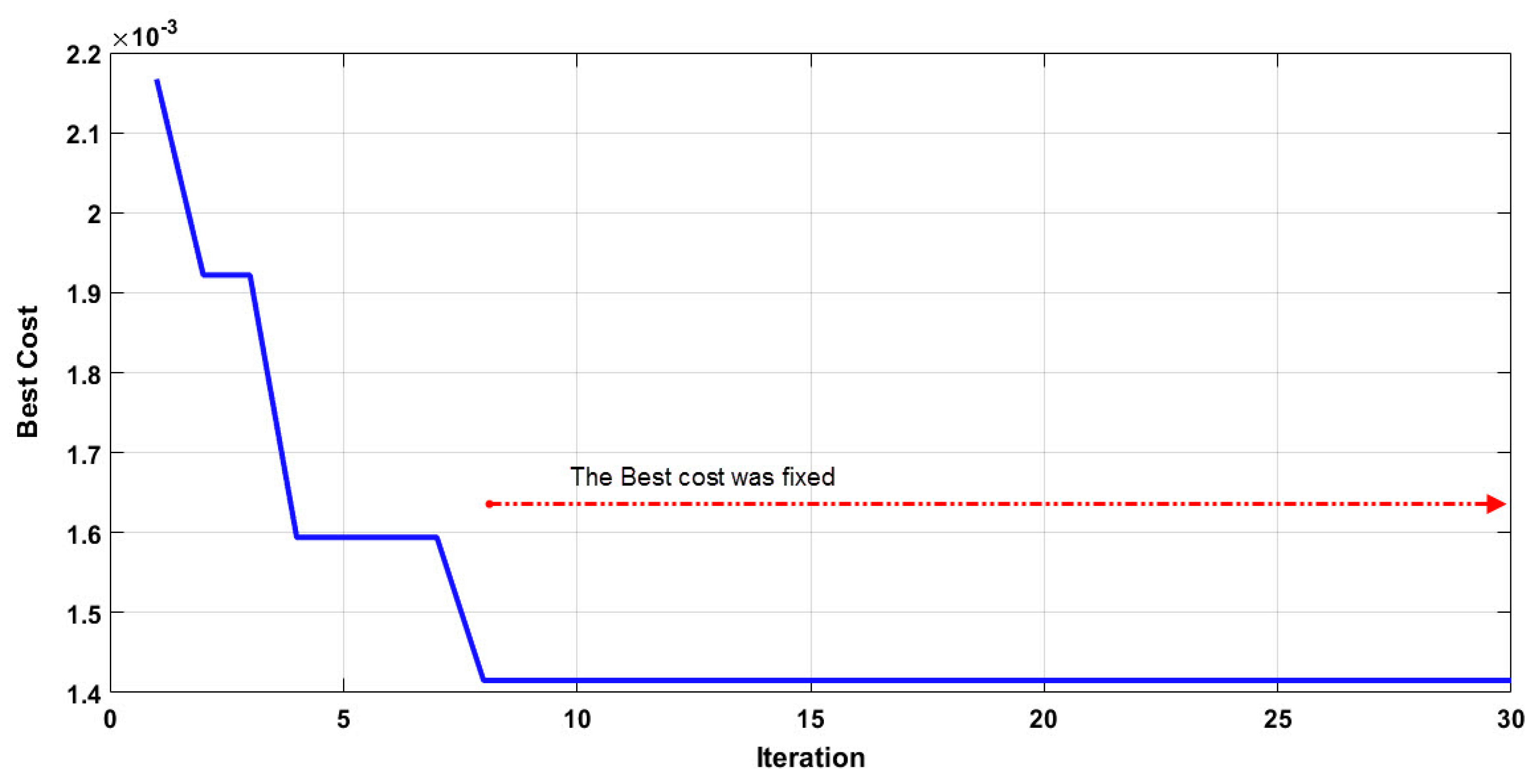
3.2. DE Modelling
4. Discussion
- Prediction of MLR y = 169.96 + 0.000284 X 1 + 0.59 X 2, R2 = 0.76
- Prediction of PLSR y = 193.26 + 0.00028 X 1 + 0.257 X 2, R2 = 0.76
5. Conclusions
Author Contributions
Funding
Conflicts of Interest
Appendix A


| X1, Average Temperature, °C | X2, Humidity, % | X3, Wind, km/h | X4, Positive Cases up to 14 Days before | X4 new (Urban Parameter) * | Y, Confirmed Cases |
|---|---|---|---|---|---|
| [Shifted 6 Days (24-Feb to 18-Mar)] | [Shifted 9 Days (21-Feb to 15-Mar)] | [Shifted 9 Days (21-Feb to 15-Mar)] | [Shifted 2 Days (28-Feb to 22-Mar)] | [Shifted 2 Days (28-Feb to 22-Mar] | [1-Mar to 24-Mar] |
| 5.2 | 72.7 | 2.9 | 10 | 1720 | 38 |
| 10.2 | 63.2 | 3.2 | 10 | 1720 | 2 |
| 7.0 | 73.4 | 3.0 | 48 | 8256 | 5 |
| 2.9 | 78.3 | 4.3 | 50 | 8600 | 26 |
| 2.7 | 78.7 | 5.1 | 55 | 9460 | 26 |
| 3.5 | 64.7 | 14.3 | 81 | 13932 | 35 |
| 4.6 | 39.6 | 13.7 | 107 | 18404 | 64 |
| 3.1 | 58.7 | 6.3 | 142 | 24424 | 153 |
| 3.8 | 49 | 3.8 | 206 | 35432 | - |
| 4.1 | 72.4 | 4.3 | 359 | 61748 | 103 |
| 4.8 | 80.6 | 4.3 | 359 | 61748 | 48 |
| 2.6 | 78.1 | 7.5 | 462 | 79464 | 79 |
| 2.5 | 51.9 | 4.9 | 510 | 87720 | 260 |
| 4.9 | 58.1 | 6.3 | 588 | 101136 | 33 |
| 5.8 | 90.0 | 5.4 | 839 | 144308 | 238 |
| 4.1 | 72.8 | 3.7 | 872 | 149984 | 405 |
| 7.2 | 48.9 | 5.2 | 1072 | 184384 | 381 |
| 9.8 | 62.6 | 4.3 | 1475 | 253700 | 444 |
| 11.0 | 70.0 | 5.0 | 1851 | 318372 | 591 |
| 9.4 | 55.0 | 4.5 | 2269 | 390268 | 529 |
| 6.6 | 74.7 | 3.6 | 2834 | 487448 | 291 |
| 7.1 | 83.4 | 3.0 | 3328 | 572416 | 668 |
| 5.8 | 84.4 | 6.7 | 3555 | 611460 | 441 |
| 7.5 | 84.2 | 3.8 | 4070 | 700040 | 654 |
| X1, Average Temperature, °C | X2, Humidity, % | X3, Wind, km/h | X4, Positive Cases up to 14 Days before | X4 new (Urban Parameter) * | Y, Confirmed Cases |
|---|---|---|---|---|---|
| [Shifted 5 Days (20-Feb to 19-Mar)] | [Shifted 8 Days (17-Feb to 16-Mar)] | [Shifted 6 Days (19-Feb to 18-Mar)] | [Shifted 4 Days (21-Feb to 20-Mar)] | [Shifted 4 Days (21-Feb to 20-Mar)] | [25-Feb to 24-Mar] |
| 7.5 | 92.2 | 5.6 | 2 | 544 | 11 |
| 7.2 | 89.9 | 6.3 | 18 | 4896 | 28 |
| 7.8 | 86.7 | 10.1 | 25 | 6800 | 40 |
| 7.4 | 74.3 | 7.9 | 32 | 8704 | 40 |
| 8.9 | 71.3 | 6.3 | 43 | 11696 | 40 |
| 9.3 | 68.2 | 7.9 | 71 | 19312 | 72 |
| 9.1 | 87.6 | 6 | 111 | 30192 | 10 |
| 8.2 | 86.4 | 10 | 151 | 41072 | 34 |
| 9.1 | 92.7 | 14.6 | 191 | 51952 | 53 |
| 7.3 | 90 | 10.7 | 263 | 71536 | 47 |
| 8.6 | 62.6 | 9 | 273 | 74256 | 81 |
| 7.1 | 52.5 | 9.7 | 307 | 83504 | 55 |
| 10 | 64.2 | 11.6 | 360 | 97920 | 127 |
| 9.1 | 79.8 | 14.8 | 407 | 110704 | 74 |
| 7.2 | 94.8 | 10.7 | 486 | 132192 | 112 |
| 7.5 | 89.8 | 5.6 | 525 | 142800 | 167 |
| 8.9 | 76.2 | 16.7 | 645 | 175440 | 361 |
| 9.4 | 72.8 | 5.3 | 712 | 193664 | 211 |
| 8.6 | 80.7 | 11.4 | 813 | 221136 | 342 |
| 9.1 | 82.5 | 7.9 | 952 | 258944 | 235 |
| 9.1 | 68 | 6.5 | 1273 | 346256 | 301 |
| 9.2 | 68.2 | 6.7 | 1444 | 392768 | 231 |
| 11.2 | 74.2 | 7.9 | 1746 | 474912 | 510 |
| 11.5 | 82.3 | 6.7 | 1909 | 519248 | 270 |
| 9 | 84.9 | 14.1 | 2200 | 598400 | 547 |
| 8.2 | 89.8 | 17.6 | 2397 | 651984 | 586 |
| 9 | 73.8 | 9.3 | 2854 | 776288 | 505 |
| 11.1 | 64.3 | 7.2 | 3077 | 836944 | 383 |
| 14.2 | 52.6 | 7.2 | 3543 | 963696 | 443 |
| X1, Average Temperature, °C | X2, Humidity, % | X3, Wind, km/h | X4, Positive Cases up to 14 Days before | X4 new (Urban Parameter) * | Y, Confirmed Cases |
|---|---|---|---|---|---|
| [Shifted 8 days (17-Feb to 16-Mar)] | [Shifted 6 days (19-Feb to 18-Mar)] | [Shifted 8 days (17-Feb to 16-Mar)] | [Shifted 3 days (22-Feb to1-Mar)] | [Shifted 3 days (22-Feb to1-Mar)] | [25-Feb to 24-Mar] |
| 8.8 | 83.3 | 5.6 | 2 | 398 | 8 |
| 11.5 | 72.9 | 6.5 | 9 | 1791 | 21 |
| 10.2 | 74 | 6.3 | 18 | 3582 | 50 |
| 8.0 | 74.2 | 7.6 | 26 | 5174 | 48 |
| 9 | 73.2 | 4.3 | 47 | 9353 | 72 |
| 7.2 | 77.6 | 5.3 | 97 | 19303 | 68 |
| 8.8 | 84.3 | 7.4 | 145 | 28855 | 50 |
| 10 | 69.6 | 4.9 | 217 | 43183 | 85 |
| 9.8 | 33.6 | 5.8 | 285 | 56715 | 124 |
| 11.2 | 37.8 | 10.2 | 335 | 66665 | 154 |
| 8.6 | 36.1 | 20.8 | 420 | 83580 | 172 |
| 10.5 | 66.2 | 19.1 | 544 | 108256 | 140 |
| 8.6 | 90.5 | 7.2 | 698 | 138902 | 170 |
| 10 | 82.8 | 12 | 870 | 173130 | 206 |
| 6.2 | 84.9 | 7.9 | 1008 | 200592 | 147 |
| 10.3 | 69 | 14.1 | 1171 | 233029 | 206 |
| 7.5 | 82.5 | 9.7 | 1368 | 272232 | 208 |
| 7.5 | 81.3 | 8.1 | 1507 | 299893 | 316 |
| 8.5 | 74.3 | 13.9 | 1692 | 336708 | 381 |
| 8.7 | 59.9 | 10.6 | 1850 | 368150 | 449 |
| 8.8 | 70.6 | 6.7 | 2118 | 421482 | 429 |
| 8.6 | 62.9 | 7.6 | 2427 | 482973 | 409 |
| 8.1 | 61.7 | 7.4 | 2808 | 558792 | 594 |
| 9.1 | 74 | 6.3 | 3187 | 634213 | 689 |
| 11.5 | 79.6 | 8.1 | 3511 | 698689 | 754 |
| 13 | 71.1 | 5.1 | 3981 | 792219 | 737 |
| 13.2 | 56.4 | 9 | 4516 | 898684 | 850 |
| 9.2 | 54.4 | 8.3 | 5098 | 1014502 | 980 |
| 7.6 | 59 | 6.7 | 5695 | 1133305 | 719 |
Appendix B
| Date | Daily New Cases | X4 Positive Cases up to 14 Days before [Shifted 3 Days] | X4new [Population Density *X4] | Date | Daily New Cases | X4 Positive Cases up to 14 Days before [Shifted 3 Days] | X4new [Population Density *X4] |
|---|---|---|---|---|---|---|---|
| 20-Feb | 0 | 0 | 0 | 04-Apr | 1598 | 27060 | 11419320 |
| 21-Feb | 15 | 0 | 0 | 05-Apr | 1337 | 26181 | 11048382 |
| 22-Feb | 40 | 0 | 0 | 06-Apr | 1079 | 25256 | 10658032 |
| 23-Feb | 57 | 0 | 0 | 07-Apr | 791 | 23603 | 9960466 |
| 24-Feb | 61 | 15 | 6330 | 08-Apr | 1089 | 23249 | 9811078 |
| 25-Feb | 67 | 55 | 23210 | 09-Apr | 1388 | 22773 | 9610206 |
| 26-Feb | 65 | 112 | 47264 | 10-Apr | 1246 | 21622 | 9124484 |
| 27-Feb | 98 | 173 | 73006 | 11-Apr | 1544 | 21068 | 8890696 |
| 28-Feb | 128 | 240 | 101280 | 12-Apr | 1460 | 19913 | 8403286 |
| 29-Feb | 84 | 305 | 128710 | 13-Apr | 1262 | 18750 | 7912500 |
| 01-Mar | 369 | 403 | 170066 | 14-Apr | 1012 | 18177 | 7670694 |
| 02-Mar | 270 | 531 | 224082 | 15-Apr | 827 | 18045 | 7614990 |
| 03-Mar | 266 | 615 | 259530 | 16-Apr | 941 | 18153 | 7660566 |
| 04-Mar | 300 | 984 | 415248 | 17-Apr | 1041 | 18118 | 7645796 |
| 05-Mar | 431 | 1254 | 529188 | 18-Apr | 1246 | 17380 | 7334360 |
| 06-Mar | 361 | 1520 | 641440 | 19-Apr | 855 | 17029 | 7186238 |
| 07-Mar | 808 | 1820 | 768040 | 20-Apr | 735 | 16615 | 7011530 |
| 08-Mar | 769 | 2251 | 949922 | 21-Apr | 960 | 16263 | 6862986 |
| 09-Mar | 1280 | 2597 | 1095934 | 22-Apr | 1161 | 15781 | 6659582 |
| 10-Mar | 322 | 3365 | 1420030 | 23-Apr | 1073 | 15437 | 6514414 |
| 11-Mar | 1489 | 4077 | 1720494 | 24-Apr | 1091 | 15606 | 6585732 |
| 12-Mar | 1445 | 5296 | 2234912 | 25-Apr | 713 | 15678 | 6616116 |
| 13-Mar | 1095 | 5551 | 2342522 | 26-Apr | 920 | 15363 | 6483186 |
| 14-Mar | 1865 | 6975 | 2943450 | 27-Apr | 590 | 15208 | 6417776 |
| 15-Mar | 1587 | 8322 | 3511884 | 28-Apr | 869 | 14377 | 6067094 |
| 16-Mar | 1377 | 9289 | 3919958 | 29-Apr | 786 | 13837 | 5839214 |
| 17-Mar | 1571 | 11070 | 4671540 | 30-Apr | 598 | 13165 | 5555630 |
| 18-Mar | 1493 | 12288 | 5185536 | 01-May | 737 | 13022 | 5495284 |
| 19-Mar | 2171 | 13395 | 5652690 | 02-May | 533 | 12981 | 5477982 |
| 20-Mar | 2380 | 14700 | 6203400 | 03-May | 526 | 12638 | 5333236 |
| 21-Mar | 3251 | 15893 | 6706846 | 04-May | 577 | 12334 | 5204948 |
| 22-Mar | 1691 | 17633 | 7441126 | 05-May | 500 | 11621 | 4904062 |
| 23-Mar | 1555 | 19652 | 8293144 | 06-May | 764 | 11292 | 4765224 |
| 24-Mar | 1942 | 22095 | 9324090 | 07-May | 720 | 11134 | 4698548 |
| 25-Mar | 1643 | 23017 | 9713174 | 08-May | 634 | 10674 | 4504428 |
| 26-Mar | 2543 | 23292 | 9829224 | 09-May | 502 | 10277 | 4336894 |
| 27-Mar | 2409 | 24912 | 10512864 | 10-May | 282 | 9924 | 4187928 |
| 28-Mar | 2117 | 25066 | 10577852 | 11-May | 364 | 9467 | 3995074 |
| 29-Mar | 1592 | 26164 | 11041208 | 12-May | 1033 | 9256 | 3906032 |
| 30-Mar | 1154 | 27478 | 11595716 | 13-May | 394 | 8618 | 3636796 |
| 31-Mar | 1047 | 27730 | 11702060 | 14-May | 522 | 8392 | 3541424 |
| 01-Apr | 1565 | 27735 | 11704170 | 15-May | 299 | 8556 | 3610632 |
| 02-Apr | 1292 | 27512 | 11610064 | 16-May | 399 | 8164 | 3445208 |
| 03-Apr | 1455 | 26988 | 11388936 | 17-May | 326 | 8088 | 3413136 |

References
- Kates, R.W.; Parris, T.M.; Leiserowitz, A.A. What is sustainable development? Goals, indicators, values, and practice. Environment 2005, 47, 8–21. [Google Scholar] [CrossRef]
- Blewitt, J. Understanding Sustainable Development; Abingdon upon Thames: Routledge, UK, 2012; ISBN 9781849773645. [Google Scholar]
- Carbone, M.; Garofalo, G.; Nigro, G.; Piro, P. A conceptual model for predicting hydraulic behaviour of a green roof. Procedia Eng. 2014, 70, 266–274. [Google Scholar] [CrossRef]
- Sustainable Development Goals. Available online: https://sustainabledevelopment.un.org/?menu=1300 (accessed on 14 April 2020).
- Chen, D.; Schudeleit, T.; Posselt, G.; Thiede, S. A state-of-the-art review and evaluation of tools for factory sustainability assessment. Procedia Cirp 2013, 9, 85–90. [Google Scholar] [CrossRef]
- Jayal, A.D.; Badurdeen, F.; Dillon, O.W., Jr.; Jawahir, I.S. Sustainable manufacturing: Modeling and optimization challenges at the product, process and system levels. Cirp J. Manuf. Sci. Technol. 2010, 2, 144–152. [Google Scholar] [CrossRef]
- Maiolo, M.; Carini, M.; Capano, G.; Piro, P. Synthetic sustainability index (SSI) based on life cycle assessment approach of low impact development in the Mediterranean area. Cogent Eng. 2017, 4, 1410272. [Google Scholar] [CrossRef]
- Piro, P.; Turco, M.; Palermo, S.A.; Principato, F.; Brunetti, G. A Comprehensive Approach to Stormwater Management Problems in the Next Generation Drainage Networks. In The Internet of Things for Smart Urban Ecosystems; Springer: Cham, Switzerland, 2019; pp. 275–304. [Google Scholar] [CrossRef]
- Pirouz, B.; Arcuri, N.; Pirouz, B.; Palermo, S.A.; Turco, M.; Maiolo, M. Development of an assessment method for evaluation of sustainable factories. Sustainability 2020, 12, 1841. [Google Scholar] [CrossRef]
- Piro, P.; Carbone, M.; Garofalo, G.; Sansalone, J. CSO treatment strategy based on constituent index relationships in a highly urbanised catchment. Water Sci. Technol. 2007, 56, 85–91. [Google Scholar] [CrossRef]
- Palermo, S.A.; Talarico, V.C.; Pirouz, B. Optimizing Rainwater Harvesting Systems for Non-potable Water Uses and Surface Runoff Mitigation. In Numerical Computations: Theory and Algorithms. NUMTA 2019; Sergeyev, Y., Kvasov, D., Eds.; Lecture Notes in Computer Science; Springer: Cham, Switzerland, 2020; Volume 11973, pp. 570–582. [Google Scholar] [CrossRef]
- Pirouz, B.; Maiolo, M. The Role of Power Consumption and Type of Air Conditioner in Direct and Indirect Water Consumption. J. Sustain. Dev. Energy Water Environ. Syst. 2018, 6, 665–673. [Google Scholar] [CrossRef]
- Maiolo, M.; Pirouz, B.; Bruno, R.; Palermo, S.A.; Arcuri, N.; Piro, P. The Role of the Extensive Green Roofs on Decreasing Building Energy Consumption in the Mediterranean Climate. Sustainability 2020, 12, 359. [Google Scholar] [CrossRef]
- Pirouz, B.; Arcuri, N.; Maiolo, M.; Talarico, V.C.; Piro, P. A new multi-objective dynamic model to close the gaps in sustainable development of industrial sector. In IOP Conference Series: Earth and Environmental Science; IOP Publishing: Thessaloniki, Greece, 2020; Volume 410, p. 012074. [Google Scholar] [CrossRef]
- Pirouz, B.; Golmohammadi, A.; Saeidpour Masouleh, H.; Violini, G.; Pirouz, B. Relationship between average daily temperature and average cumulative daily rate of confirmed cases of COVID-19. medRixv 2020. [Google Scholar] [CrossRef]
- Pirouz, B.; Haghshenas, S.S.; Pirouz, B.; Haghshenas, S.S.; Piro, P. Development of an Assessment Method for Investigating the Impact of Climate and Urban Parameters in Confirmed Cases of COVID-19: A New Challenge in Sustainable Development. Int. J. Environ. Res. Public Health 2020. [Google Scholar] [CrossRef] [PubMed]
- Palermo, S.A.; Zischg, J.; Sitzenfrei, R.; Rauch, W.; Piro, P. Parameter Sensitivity of a Microscale Hydrodynamic Model. In New Trends in Urban Drainage Modelling. UDM 2018; Mannina, G., Ed.; Green Energy and Technology; Springer: Cham, Switzerland, 2019; pp. 982–987. [Google Scholar] [CrossRef]
- Giordano, A.; Spezzano, G.; Vinci, A.; Garofalo, G.; Piro, P. A Cyber-Physical System for Distributed Real-Time Control of Urban Drainage Networks in Smart Cities. In Internet and Distributed Computing Systems. IDCS 2014; Fortino, G., Di Fatta, G., Li, W., Ochoa, S., Cuzzocrea, A., Pathan, M., Eds.; Lecture Notes in Computer Science; Springer: Cham, Switzerland, 2014; Volume 8729, pp. 87–98. [Google Scholar] [CrossRef]
- Piro, P.; Carbone, M.; Morimanno, F.; Palermo, S.A. Simple flowmeter device for LID systems: From laboratory procedure to full-scale implementation. Flow Meas. Instrum. 2019, 65, 240–249. [Google Scholar] [CrossRef]
- Carbone, M.; Turco, M.; Brunetti, G.; Piro, P. A Cumulative Rainfall Function for Subhourly Design Storm in Mediterranean Urban Areas. Adv. Meteorol. 2015. [Google Scholar] [CrossRef]
- World Health Organization (WHO). Coronavirus Disease (COVID-2019) Situation Reports. Available online: https://www.who.int/emergencies/diseases/novel-coronavirus-2019/situation-reports/ (accessed on 28 March 2020).
- Cascella, M.; Rajnik, M.; Cuomo, A.; Dulebohn, S.C.; Di Napoli, R. Features, Evaluation and Treatment Coronavirus (COVID-19); StatPearls Publishing LLC: Tampa, FL, USA, 2020; Available online: https://www.ncbi.nlm.nih.gov/books/NBK554776/ (accessed on 29 March 2020).
- Shen, M.; Peng, Z.; Guo, Y.; Xiao, Y.; Zhang, L. Lockdown may partially halt the spread of 2019 novel coronavirus in Hubei province, China. medRxiv 2020. [Google Scholar] [CrossRef]
- Phan, L.T.; Nguyen, T.V.; Luong, Q.C.; Nguyen, T.V.; Nguyen, H.T.; Le, H.Q.; Nguyen, T.T.; Cao, T.M.; Pham, Q.D. Importation and human-to-human transmission of a novel coronavirus in Vietnam. N. Engl. J. Med. 2020, 382, 872–874. [Google Scholar] [CrossRef]
- Gilbert, M.; Pullano, G.; Pinotti, F.; Valdano, E.; Poletto, C.; Boëlle, P.Y.; D’Ortenzio, E.; Yazdanpanah, Y.; Eholie, S.P.; Gutierrez, B.; et al. Preparedness and vulnerability of African countries against importations of COVID-19: A modelling study. Lancet 2020, 395, 871–877. [Google Scholar] [CrossRef]
- Yu, H.; Sun, X.; Solvang, W.D.; Zhao, X. Reverse Logistics Network Design for Effective Management of Medical Waste in Epidemic Outbreaks: Insights from the Coronavirus Disease 2019 (COVID-19) Outbreak in Wuhan (China). Int. J. Environ. Res. Public Health 2020, 17, 1770. [Google Scholar] [CrossRef]
- Chen, Y.C.; Lu, P.E.; Chang, C.S. A Time-dependent SIR model for COVID-19. arXiv 2020, arXiv:2003.00122. [Google Scholar]
- Pirouz, B.; Shaffiee Haghshenas, S.; Shaffiee Haghshenas, S.; Piro, P. Investigating a Serious Challenge in the Sustainable Development Process: Analysis of Confirmed cases of COVID-19 (New Type of Coronavirus) Through a Binary Classification Using Artificial Intelligence and Regression Analysis. Sustainability 2020, 12, 2427. [Google Scholar] [CrossRef]
- Hu, Z.; Ge, Q.; Jin, L.; Xiong, M. Artificial intelligence forecasting of covid-19 in china. arXiv 2020, arXiv:2002.07112. [Google Scholar]
- Kampf, G.; Todt, D.; Pfaender, S.; Steinmann, E. Persistence of coronaviruses on inanimate surfaces and its inactivation with biocidal agents. J. Hosp. Infect. 2020, 104, 246–251. [Google Scholar] [CrossRef] [PubMed]
- Grant, W.B.; Giovannucci, E. The possible roles of solar ultraviolet-B radiation and vitamin D in reducing case-fatality rates from the 1918–1919 influenza pandemic in the United States. Derm. Endocrinol. 2009, 1, 215–219. [Google Scholar] [CrossRef] [PubMed]
- Chan, K.H.; Peiris, J.S.; Lam, S.Y.; Poon, L.L.; Yuen, K.Y.; Seto, W.H. The effects of temperature and relative humidity on the viability of the SARS coronavirus. Adv. Virol. 2011. [Google Scholar] [CrossRef] [PubMed]
- Coronavirus Incubation Period. Available online: https://www.worldometers.info/coronavirus/coronavirus-incubation-period/#24 (accessed on 27 March 2020).
- Coronavirus Testing: How it Is Done, When you Should Get One and How Long Results Take. Available online: https://www.liverpoolecho.co.uk/news/uk-world-news/coronavirus-testing-how-done-you-17912266 (accessed on 27 March 2020).
- Li, Q.; Guan, X.; Wu, P.; Wang, X.; Zhou, L.; Tong, Y.; Ren, R.; Leung, K.S.M.; Lau, E.H.Y.; Xing, X.; et al. Early Transmission Dynamics in Wuhan, China, of Novel Coronavirus–Infected Pneumonia. N. Engl. J. Med. 2020. [Google Scholar] [CrossRef]
- Coronavirus Testing: Information on COVID-19 Tests According to State Health Departments. Available online: https://www.nbcnews.com/health/health-news/coronavirus-testing-information-covid-19-tests-according-state-health-departments-n1158041 (accessed on 25 March 2020).
- In Italia ieri Record Mondiale di Decessi. Rebus Lombardia. Available online: https://ilmanifesto.it/in-italia-ieri-record-mondiale-di-decessi-rebus-lombardia/ (accessed on 26 March 2020).
- Coronavirus Cases. Available online: https://www.worldometers.info/coronavirus/ (accessed on 26 March 2020).
- Mikaeil, R.; Haghshenas, S.S.; Hoseinie, S.H. Rock penetrability classification using artificial bee colony (ABC) algorithm and self-organizing map. Geotech. Geol. Eng. 2018, 36, 1309–1318. [Google Scholar] [CrossRef]
- Naderpour, H.; Mirrashid, M. Moment capacity estimation of spirally reinforced concrete columns using ANFIS. Complex Intell. Syst. 2019, 1–11. [Google Scholar] [CrossRef]
- Naderpour, H.; Mirrashid, M. Shear failure capacity prediction of concrete beam–column joints in terms of ANFIS and GMDH. Pract. Period. Struct. Des. Constr. 2019, 24, 04019006. [Google Scholar] [CrossRef]
- Kayabekir, A.E.; Toklu, Y.C.; Bekdaş, G.; Nigdeli, S.M.; Yücel, M.; Geem, Z.W. A Novel Hybrid Harmony Search Approach for the Analysis of Plane Stress Systems via Total Potential Optimization. Appl. Sci. 2020, 10, 2301. [Google Scholar] [CrossRef]
- Na, K.S.; Cho, S.E.; Geem, Z.W.; Kim, Y.K. Predicting future onset of depression among community dwelling adults in the Republic of Korea using a machine learning algorithm. Neurosci. Lett. 2020, 721, 134804. [Google Scholar] [CrossRef]
- Kandiri, A.; Golafshani, E.M.; Behnood, A. Estimation of the compressive strength of concretes containing ground granulated blast furnace slag using hybridized multi-objective ANN and salp swarm algorithm. Constr. Build. Mater. 2020, 248, 118676. [Google Scholar] [CrossRef]
- Geem, Z.W. Transport energy demand modeling of South Korea using artificial neural network. Energy Policy 2011, 39, 4644–4650. [Google Scholar] [CrossRef]
- Rad, M.Y.; Haghshenas, S.S.; Kanafi, P.R.; Haghshenas, S.S. Analysis of Protection of Body Slope in the Rockfill Reservoir Dams on the Basis of Fuzzy Logic. In Proceedings of the 4th International Joint Conference on Computational Intelligence, Barcelona, Spain, 5–7 October 2012; pp. 367–373. [Google Scholar]
- Rad, M.Y.; Haghshenas, S.S.; Haghshenas, S.S. Mechanostratigraphy of cretaceous rocks by fuzzy logic in East Arak, Iran. In Proceedings of the 4th International Workshop on Computer Science and Engineering-Summer, WCSE, Dubai, 22–23 August 2014. [Google Scholar]
- Mikaeil, R.; Haghshenas, S.S.; Haghshenas, S.S.; Ataei, M. Performance prediction of circular saw machine using imperialist competitive algorithm and fuzzy clustering technique. Neural Comput. Appl. 2018, 29, 283–292. [Google Scholar] [CrossRef]
- Dormishi, A.; Ataei, M.; Mikaeil, R.; Khalokakaei, R.; Haghshenas, S.S. Evaluation of gang saws’ performance in the carbonate rock cutting process using feasibility of intelligent approaches. Eng. Sci. Technol. Int. J. 2019, 22, 990–1000. [Google Scholar] [CrossRef]
- Mikaeil, R.; Beigmohammadi, M.; Bakhtavar, E.; Haghshenas, S.S. Assessment of risks of tunneling project in Iran using artificial bee colony algorithm. SN Appl. Sci. 2019, 1, 1711. [Google Scholar] [CrossRef]
- Behnood, A.; Golafshani, E.M. Machine learning study of the mechanical properties of concretes containing waste foundry sand. Constr. Build. Mater. 2020, 243, 118152. [Google Scholar] [CrossRef]
- Cabaneros, S.M.S.; Calautit, J.K.; Hughes, B.R. A review of artificial neural network models for ambient air pollution prediction. Environ. Model. Softw. 2019, 119, 285–304. [Google Scholar] [CrossRef]
- Maleki, H.; Sorooshian, A.; Goudarzi, G.; Baboli, Z.; Birgani, Y.T.; Rahmati, M. Air pollution prediction by using an artificial neural network model. Clean Technol. Environ. Policy 2019, 21, 1341–1352. [Google Scholar] [CrossRef]
- Araujo, L.N.; Belotti, J.T.; Alves, T.A.; de Souza Tadano, Y.; Siqueira, H. Ensemble method based on Artificial Neural Networks to estimate air pollution health risks. Environ. Model. Softw. 2020, 123, 104567. [Google Scholar] [CrossRef]
- Mahdevari, S.; Shahriar, K.; Sharifzadeh, M.; Tannant, D.D. Stability prediction of gate roadways in longwall mining using artificial neural networks. Neural Comput. Appl. 2017, 28, 3537–3555. [Google Scholar] [CrossRef]
- Naderpour, H.; Poursaeidi, O.; Ahmadi, M. Shear resistance prediction of concrete beams reinforced by FRP bars using artificial neural networks. Measurement 2018, 126, 299–308. [Google Scholar] [CrossRef]
- Mohammadi, J.; Ataei, M.; Kakaei, R.K.; Mikaeil, R.; Haghshenas, S.S. Prediction of the production rate of chain saw machine using the multilayer perceptron (MLP) neural network. Civ. Eng. J. 2018, 4, 1575–1583. [Google Scholar] [CrossRef]
- Mikaeil, R.; Haghshenas, S.S.; Ozcelik, Y.; Gharehgheshlagh, H.H. Performance evaluation of adaptive neuro-fuzzy inference system and group method of data handling-type neural network for estimating wear rate of diamond wire saw. Geotech. Geol. Eng. 2018, 36, 3779–3791. [Google Scholar] [CrossRef]
- Genc, O.; Kisi, O.; Ardiclioglu, M. Modeling velocity distributions in small streams using different neuro-fuzzy and neural computing techniques. J. Water Clim. Chang. 2019. [Google Scholar] [CrossRef]
- Faris, H.; Aljarah, I.; Mirjalili, S. Improved monarch butterfly optimization for unconstrained global search and neural network training. Appl. Intell. 2018, 48, 445–464. [Google Scholar] [CrossRef]
- Noori, A.M.; Mikaeil, R.; Mokhtarian, M.; Haghshenas, S.S.; Foroughi, M. Feasibility of intelligent models for prediction of utilization factor of TBM. Geotech. Geol. Eng. 2020, 1–19. [Google Scholar] [CrossRef]
- Petrudi, S.H.J.; Pirouz, M.; Pirouz, B. Application of fuzzy logic for performance evaluation of academic students. In Proceedings of the 13th Iranian Conference on Fuzzy Systems (IFSC), Qazvin, Iran, 27–29 August 2013; pp. 1–5. [Google Scholar] [CrossRef]
- Karahan, H.; Gurarslan, G.; Geem, Z.W. Parameter estimation of the nonlinear Muskingum flood-routing model using a hybrid harmony search algorithm. J. Hydrol. Eng. 2013, 18, 352–360. [Google Scholar] [CrossRef]
- Haghshenas, S.S.; Haghshenas, S.S.; Mikaeil, R.; Sirati Moghadam, P.; Haghshenas, A.S. A new model for evaluating the geological risk based on geomechanical properties-case study: The second part of emamzade hashem tunnel. Electron. J. Geotech. Eng. 2017, 22, 309–320. [Google Scholar]
- Salemi, A.; Mikaeil, R.; Haghshenas, S.S. Integration of finite difference method and genetic algorithm to seismic analysis of circular shallow tunnels (Case study: Tabriz urban railway tunnels). KSCE J. Civ. Eng. 2018, 22, 1978–1990. [Google Scholar] [CrossRef]
- Haghshenas, S.S.; Faradonbeh, R.S.; Mikaeil, R.; Haghshenas, S.S.; Taheri, A.; Saghatforoush, A.; Dormishi, A. A new conventional criterion for the performance evaluation of gang saw machines. Measurement 2019, 146, 159–170. [Google Scholar] [CrossRef]
- Roohollah Shirani, F.; Haghshenas, S.S.; Taheri, A.; Mikaeil, R. Application of self-organizing map and fuzzy c-mean techniques for rockburst clustering in deep underground projects. Neural Comput. Appl. 2019, 1–15. [Google Scholar] [CrossRef]
- Mikaeil, R.; Bakhshinezhad, H.; Haghshenas, S.S.; Ataei, M. Stability analysis of tunnel support systems using numerical and intelligent simulations (case study: Kouhin Tunnel of Qazvin-Rasht Railway). Rud. Geološko Naft. Zb. 2019, 34, 1–10. [Google Scholar] [CrossRef]
- Hosseini, S.M.; Ataei, M.; Khalokakaei, R.; Mikaeil, R.; Haghshenas, S.S. Study of the effect of the cooling and lubricant fluid on the cutting performance of dimension stone through artificial intelligence models. Eng. Sci. Technol. Int. J. 2020, 23, 71–81. [Google Scholar] [CrossRef]
- Tikhamarine, Y.; Souag-Gamane, D.; Ahmed, A.N.; Kisi, O.; El-Shafie, A. Improving artificial intelligence models accuracy for monthly streamflow forecasting using grey Wolf optimization (GWO) algorithm. J. Hydrol. 2020, 582, 124435. [Google Scholar] [CrossRef]
- Pirouz, B.; Palermo, S.A.; Turco, M.; Piro, P. New Mathematical Optimization Approaches for LID Systems. In Numerical Computations: Theory and Algorithms. NUMTA 2019; Sergeyev, Y., Kvasov, D., Eds.; Lecture Notes in Computer Science; Springer: Cham, Switzerland, 2020; Volume 11973, pp. 583–595. [Google Scholar] [CrossRef]
- Ho, C.H.; Chang, P.T.; Hung, K.C.; Lin, K.P. Developing intuitionistic fuzzy seasonality regression with particle swarm optimization for air pollution forecasting. Ind. Manag. Data Syst. 2019, 119, 561–577. [Google Scholar] [CrossRef]
- Lee, C.Y.; Lee, Z.J.; Huang, J.Q.; Ye, F.L.; Ning, Z.Y.; Yang, C.F. Urban Air Quality Analysis and Forecast Based on Intelligent Algorithm with Parameter Optimization and Decision Rules. Appl. Sci. 2019, 9, 5445. [Google Scholar] [CrossRef]
- Shamshirband, S.; Hadipoor, M.; Baghban, A.; Mosavi, A.; Bukor, J.; Várkonyi-Kóczy, A.R. Developing an ANFIS-PSO model to predict mercury emissions in combustion flue gases. Mathematics 2019, 7, 965. [Google Scholar] [CrossRef]
- Wang, J.; Du, P.; Hao, Y.; Ma, X.; Niu, T.; Yang, W. An innovative hybrid model based on outlier detection and correction algorithm and heuristic intelligent optimization algorithm for daily air quality index forecasting. J. Environ. Manag. 2020, 255, 109855. [Google Scholar] [CrossRef]
- Zeinalnezhad, M.; Chofreh, A.G.; Goni, F.A.; Klemeš, J. Air pollution prediction using semi-experimental regression model and Adaptive Neuro-Fuzzy Inference System. J. Clean. Prod 2020, 121218. [Google Scholar] [CrossRef]
- Kennedy, J.; Eberhart, R. Particle swarm optimization. In Proceedings of the ICNN’95-International Conference on Neural Networks, Perth, WA, Australia, 27 November–1 December 1995; Volume 4, pp. 1942–1948. [Google Scholar] [CrossRef]
- Shi, Y. Particle swarm optimization: Developments, applications and resources. In Proceedings of the 2001 Congress on Evolutionary Computation, Seoul, Korea, 27–30 May 2001; Volume 1, pp. 81–86. [Google Scholar] [CrossRef]
- Poli, R.; Kennedy, J.; Blackwell, T. Particle swarm optimization. Swarm Intell. 2007, 1, 33–57. [Google Scholar] [CrossRef]
- Mikaeil, R.; Haghshenas, S.S.; Sedaghati, Z. Geotechnical risk evaluation of tunneling projects using optimization techniques (case study: The second part of Emamzade Hashem tunnel). Nat. Hazards 2019, 97, 1099–1113. [Google Scholar] [CrossRef]
- Karaboga, D.; Akay, B. A comparative study of artificial bee colony algorithm. Appl. Math. Comput. 2019, 214, 108–132. [Google Scholar] [CrossRef]
- Tharwat, A.; Elhoseny, M.; Hassanien, A.E.; Gabel, T.; Kumar, A. Intelligent Bézier curve-based path planning model using Chaotic Particle Swarm Optimization algorithm. Clust. Comput. 2019, 22, 4745–4766. [Google Scholar] [CrossRef]
- Aryafar, A.; Mikaeil, R.; Doulati Ardejani, F.; Shaffiee Haghshenas, S.; Jafarpour, A. Application of non-linear regression and soft computing techniques for modeling process of pollutant adsorption from industrial wastewaters. J. Min. Environ. 2019, 10, 327–337. [Google Scholar] [CrossRef]
- Storn, R.; Price, K. Differential Evolution—A Simple and Efficient Adaptive Scheme for Global Optimization over Continuous Spaces; Technical Report; International Computer Science Institute: Berkeley, CA, USA, 1995. [Google Scholar]
- Storn, R.; Price, K. Minimizing the real functions of the ICEC’96 contest by differential evolution, In Evolutionary Computation. In Proceedings of the IEEE International Conference on Evolutionary Computation, Nagoya, Japan, 20–22 May 1996; pp. 842–844. [Google Scholar] [CrossRef]
- Storn, R.; Price, K. Differential evolution–a simple and efficient heuristic for global optimization over continuous spaces. J. Glob. Optim. 1997, 11, 341–359. [Google Scholar] [CrossRef]
- Aryafar, A.; Mikaeil, R.; Haghshenas, S.S.; Haghshenas, S.S. Application of meta-heuristic algorithms to optimal clustering of sawing machine vibration. Measurement 2018, 124, 20–31. [Google Scholar] [CrossRef]
- Dehghani, H.; Shafaghi, M. Prediction of blast-induced flyrock using differential evolution algorithm. Eng. Comput. 2017, 33, 149–158. [Google Scholar] [CrossRef]
- Yang, J.; Li, W.T.; Shi, X.W.; Xin, L.; Yu, J.F. A hybrid ABC-DE algorithm and its application for time-modulated arrays pattern synthesis. IEEE Trans. Antennas Propag. 2013, 61, 5485–5495. [Google Scholar] [CrossRef]
- Wang, L.; He, J.; Wu, D.; Zeng, Y.R. A novel differential evolution algorithm for joint replenishment problem under interdependence and its application. Int. J. Prod. Econ. 2012, 135, 190–198. [Google Scholar] [CrossRef]
- Dormishi, A.R.; Ataei, M.; Khaloo Kakaie, R.; Mikaeil, R.; Shaffiee Haghshenas, S. Performance evaluation of gang saw using hybrid ANFIS-DE and hybrid ANFIS-PSO algorithms. J. Min. Environ. 2019, 10, 543–557. [Google Scholar] [CrossRef]
- AdminStat. Maps, Analysis and Statistics about the Resident Population. Available online: https://ugeo.urbistat.com/AdminStat/en/it/demografia/dati-sintesi/milano/15/3 (accessed on 27 March 2020).
- Regions of Italy. Available online: https://en.wikipedia.org/wiki/Regions_of_Italy (accessed on 27 March 2020).
- 2020 Coronavirus Pandemic in Italy. Available online: https://en.wikipedia.org/wiki/2020_coronavirus_pandemic_in_Italy#cite_note-139 (accessed on 25 March 2020).
- Lombardy. Available online: https://commons.wikimedia.org/wiki/File:Map_of_region_of_Lombardy,_Italy,_with_provinces-it.svg (accessed on 26 March 2020).
- Piedmont. Available online: https://commons.wikimedia.org/wiki/File:Map_of_region_of_Piedmont,_Italy,_with_provinces-en.svg (accessed on 26 March 2020).
- Emilia-Romagna. Available online: https://en.wikipedia.org/wiki/Emilia-Romagna#/media/File:Map_of_region_of_Emilia-Romagna,_Italy,_with_provinces-it.svg (accessed on 26 March 2020).
- Veneto. Available online: https://en.wikipedia.org/wiki/File:Map_of_region_of_Veneto,_Italy,_with_provinces-en.svg (accessed on 26 March 2020).
- Nelson, M.M.; Illingworth, W.T. A Practical Guide to Neural Nets; Addison- Wesley: Reading, MA, USA, 1991; OSTI Identifier: 5633084. [Google Scholar]
- Meteorological Conditions in the World. Available online: https://www.ogimet.com/ranking.phtml.en (accessed on 28 March 2020).
- Weather Forecast. Available online: https://yandex.com/weather/bologna/month/february (accessed on 28 March 2020).


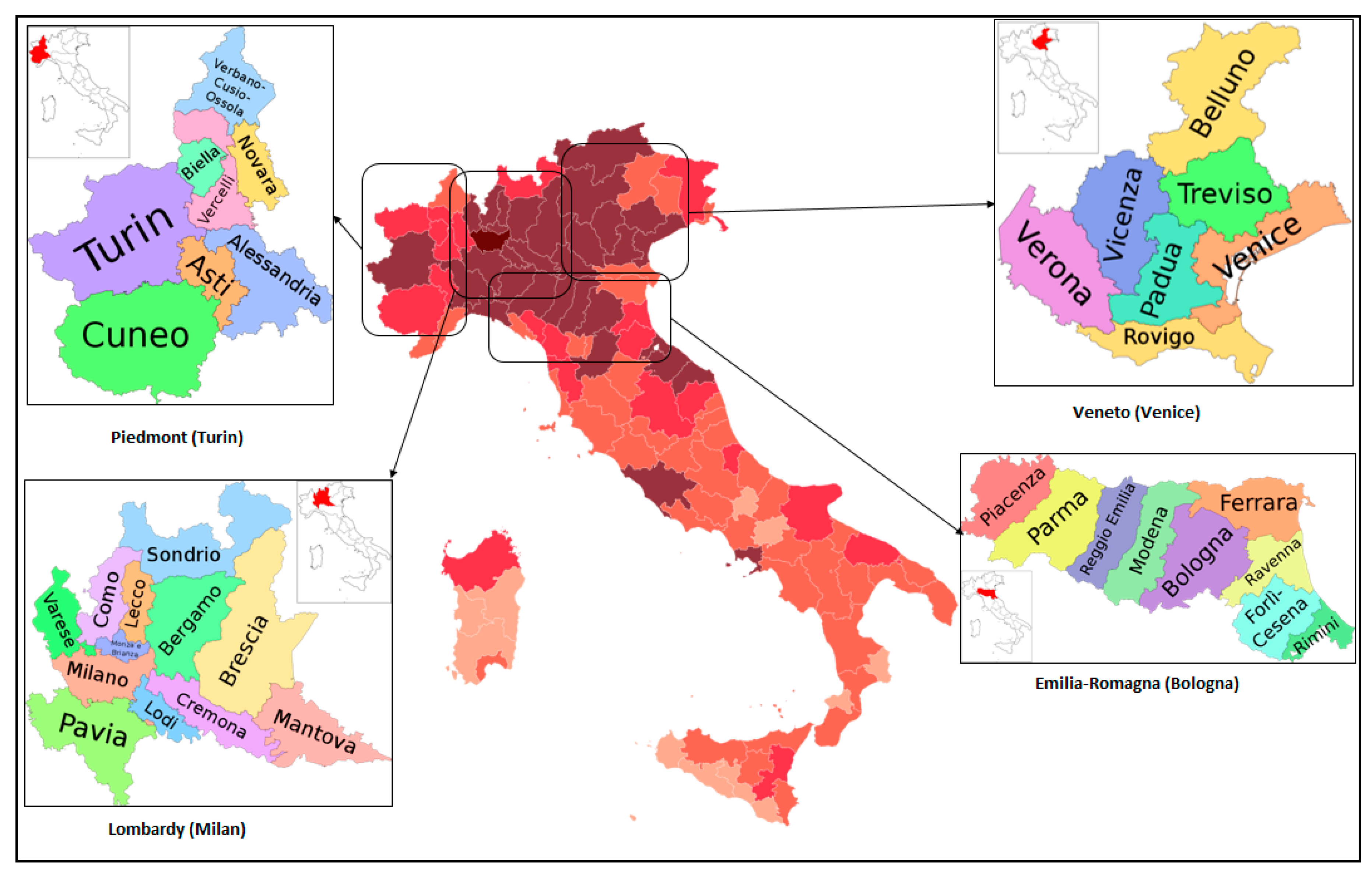
| Case Study | Population [92] | Density, Population/km2 [93] | Total Confirmed Cases Until 24th March [94] |
|---|---|---|---|
| Lombardy (Milan) | 10,060,574 | 422 | 30,703 |
| Veneto (Venice) | 4,905,854 | 272 | 5948 |
| Piedmont (Turin) | 4,356,406 | 172 | 5524 |
| Emilia-Romagna (Bolonia) | 4,459,477 | 199 | 9254 |
| Control Parameters | Values |
|---|---|
| Number of hidden layers | 10 |
| Swarm size | 15 |
| Individual learning factor (C1) | 1.49 |
| Social learning factor (C2) | 1.49 |
| Maximum number of iterations | 30 |
© 2020 by the authors. Licensee MDPI, Basel, Switzerland. This article is an open access article distributed under the terms and conditions of the Creative Commons Attribution (CC BY) license (http://creativecommons.org/licenses/by/4.0/).
Share and Cite
Shaffiee Haghshenas, S.; Pirouz, B.; Shaffiee Haghshenas, S.; Pirouz, B.; Piro, P.; Na, K.-S.; Cho, S.-E.; Geem, Z.W. Prioritizing and Analyzing the Role of Climate and Urban Parameters in the Confirmed Cases of COVID-19 Based on Artificial Intelligence Applications. Int. J. Environ. Res. Public Health 2020, 17, 3730. https://doi.org/10.3390/ijerph17103730
Shaffiee Haghshenas S, Pirouz B, Shaffiee Haghshenas S, Pirouz B, Piro P, Na K-S, Cho S-E, Geem ZW. Prioritizing and Analyzing the Role of Climate and Urban Parameters in the Confirmed Cases of COVID-19 Based on Artificial Intelligence Applications. International Journal of Environmental Research and Public Health. 2020; 17(10):3730. https://doi.org/10.3390/ijerph17103730
Chicago/Turabian StyleShaffiee Haghshenas, Sina, Behrouz Pirouz, Sami Shaffiee Haghshenas, Behzad Pirouz, Patrizia Piro, Kyoung-Sae Na, Seo-Eun Cho, and Zong Woo Geem. 2020. "Prioritizing and Analyzing the Role of Climate and Urban Parameters in the Confirmed Cases of COVID-19 Based on Artificial Intelligence Applications" International Journal of Environmental Research and Public Health 17, no. 10: 3730. https://doi.org/10.3390/ijerph17103730
APA StyleShaffiee Haghshenas, S., Pirouz, B., Shaffiee Haghshenas, S., Pirouz, B., Piro, P., Na, K.-S., Cho, S.-E., & Geem, Z. W. (2020). Prioritizing and Analyzing the Role of Climate and Urban Parameters in the Confirmed Cases of COVID-19 Based on Artificial Intelligence Applications. International Journal of Environmental Research and Public Health, 17(10), 3730. https://doi.org/10.3390/ijerph17103730