Article

Ecosystem Services and Their Driving Forces in the Middle Reaches of the Yangtze River Urban Agglomerations, China

1
Department of Geography, School of Geography and Information Engineering, China University of Geosciences, No. 388 Lumo Road, Wuhan 430074, China
2
Department of Agricultural Economics, Sociology, and Education, Population Research Institute, and Social Science Research Institute, The Pennsylvania State University, 112E Armsby, University Park, PA 16802, USA
3
Department of Land Resource Management, School of Public Administration, China University of Geosciences, Wuhan 430074, China
*
Authors to whom correspondence should be addressed.
Int. J. Environ. Res. Public Health 2020, 17(10), 3717; https://doi.org/10.3390/ijerph17103717
Submission received: 22 January 2020 / Revised: 2 February 2020 / Accepted: 3 February 2020 / Published: 25 May 2020

Abstract

:
The impact of human activities on ecosystems can be measured by ecosystem services. The study of ecosystem services is an essential part of coupled human and natural systems. However, there is limited understanding about the driving forces of ecosystem services, especially from a spatial perspective. This study attempts to fill the gap by examining the driving forces of ecosystem services with an integrated spatial approach. The results indicate that more than US$430 billion of ecosystem services value (ESV) is produced annually in the Middle Reaches of the Yangtze River Urban Agglomerations (MRYRUA), with forestland providing the largest proportion of total ESV (≥75%) and hydrological regulation function accounting for the largest proportion of total ESV (≥15%). The average ESV in the surrounding areas is obviously higher than those in the metropolitan areas, in the plains areas, and along major traffic routes. Spatial dependence and spatial spillover effects were observed in the ecosystem services in the MRYRUA. Spatial regression results indicate that road density, proportion of developed land, and river density are negatively associated with ecosystem services, while distance to a socioeconomic center, proportion of forestland land, elevation, and precipitation are positively associated with ecosystem services. The findings in this study suggest that these driving factors and the spillover effect should be taken into consideration in ecosystem protection and land-use policymaking in urban agglomerations.

1. Introduction

Urban agglomerations in China have become the main spatial carrier of urbanization [1]. Human activities in urban agglomerations have increasingly intensified land-use/land-cover change (LULCC) and exacerbated the evolution of ecosystem services [2,3]. Clearly identifying the evolutionary mechanisms of ecosystem services in urban agglomerations carries great significance for policy implications in land-use planning and ecosystem management. However, there is limited understanding about the determinants of ecosystem services from a spatial perspective. Within this context, it is crucial to characterize the spatial pattern of ecosystem services and explore their driving forces in urban agglomerations.
More specifically, an accurate assessment of ecosystem services is the foundation for studying the evolutionary mechanisms of ecosystem services, yet the assessment of ecosystem services and the study of the evolutionary mechanisms of ecosystem services in the emerging urban agglomerations in China remains incomplete. The Middle Reaches of the Yangtze River Urban Agglomerations (MRYRUA), an emerging urban agglomeration in China composed of the Wuhan metropolis, the Changsha–Zhuzhou–Xiangtan metropolis, and the Poyang Lake city group, was selected as the study area to explore land-use features and identify the driving forces of ecosystem services with spatial regression models. Geographically, the MRYRUA is located at the intersection of the east–west and north–south development axes of China, and it is an important economic center. The Yangtze River Middle Reach City Group Development Plan, implemented in 2015, proposed a strategic positioning for building a new growth pole for China’s economic development, a new type of urbanization leading zone in central and western China, an inland open cooperation demonstration zone, and a “two-type” (resource-saving and environmentally friendly society) social construction leading zone in China [4]. Thus, it is beneficial to examine the evolutionary mechanism of ecosystem services in this fast-developing urban agglomeration. To that end, this study has three specific research aims: To explore the spatiotemporal features of LULCC and the spatial pattern of ecosystem services in the MRYRUA from 1995 to 2015; to examine the driving forces of ecosystem services based on spatial aspects; and then to explain related policy implications based on the spillover effect found in this study.
The term “Ecosystem Services” was first proposed by Ehrlich and Ehrlich (1981) based on the concept of “Environmental Services” proposed by Carroll and Wilson (1970) and the concept of “Natural Services” proposed by Westman (1977) [5,6,7]. Although there is not a uniform definition of ecosystem services, the general consensus is that ecosystem services are the benefits obtained by human beings from ecosystems; that the natural ecosystems and the resources needed for human survival and development ultimately come from natural ecosystems, the subject of ecosystem services; and that ecosystem services are reflected by the conditions and processes of the ecosystem itself [6,7]. The increasing demand for ecosystem services but the scarcity of ecosystem services has brought up increasing attention to define and estimate the value of ecosystem services. One way is to monetize these tangible or intangible natural capitals, which can reflect the value brought by ecosystem services and provide the basis reference for management decisions.
The ecosystem services classification and assessment framework proposed by Costanza et al. (1997) has pushed ecosystem services research into a new phase [8]. An increasing number of comprehensive ecosystem services studies concerning ecosystem services assessment, evolutionary mechanism, trade-offs and synergies, flows, and budgets have previously been carried out [9,10,11,12]. However, there is still work to be done in the study of ecosystem services [13]. For example, the existing literature about the driving forces of ecosystem services usually ignores the spatial dependence and spatial spillover effects. However, ecosystem services in one unit are influenced by individual elements as well as by the provision capacity of ecosystem services in neighboring spatial units; that is, ecosystem services in one unit are likely to deteriorate if the ecosystem services in surrounding units deteriorate [14]. Considering only individual elements may miss or distort the truth of the evolutionary mechanism of ecosystem services. To date, the binary logistic regression model [15], gray correlation analysis [16], and ordination analysis [17] have been widely used to examine the driving forces of ecosystem services, while only a few studies identified the spatial determinant of ecosystem services with spatial regression models [9,10]. In an increasingly connected world, the spatial interaction features of ecosystem services and spatial determinants provide important information about the coordinated management of cross-regional land use and ecological protection in urban agglomerations. Thus, the spatial autocorrelations and spatial spillover effects should be taken into consideration in understanding the driving factors of ecosystem services.
The evolution of regional ecosystem services takes place under the combined influences of physical, human, and neighborhood factors, as well as land-use policy and planning [16,17,18,19]. Physical elements, such as elevation, hydrological conditions, and climate, have dominant influences on the spatial distribution pattern of ecosystem services [20,21]. The provision capacity of ecosystem services varies substantially at different elevations by different hydrological conditions and climate [22,23]. However, we live on an increasingly human-dominated planet, and the impact of human activities on the terrestrial ecosystem has dramatically exceeded those of the physical elements [24]. The human factors affecting the evolution of ecosystem services are both direct and indirect. The chief direct factors are land-use change [25], afforestation [26], deforestation [27], and land reclamation [28], among others. The primary indirect factors include urbanization [29,30], economic growth [16], population migration [31,32], traffic accessibility [33], and land-use policies [34].
Urbanization is a complex process, as are economic agglomeration, population agglomeration, and the increased demand for developed land and ecological land in urban areas [35]. Urbanization-led LULCC has profoundly transformed ecosystem services [3] and the proportion of developed land should be an essential consideration in the evolution of ecosystem services. High population density and intense economic activities in urban areas have resulted in large-scale modification of ecosystem services [36]. The construction of infrastructure, such as highways and railways, promotes economic growth and population migration [37], thereby affecting LULCC and the provisioning capacity of ecosystem services. Proximity factors, such as distance to city centers, are closely associated with other socioeconomic factors that should also be considered [38].

2. Materials and Methods

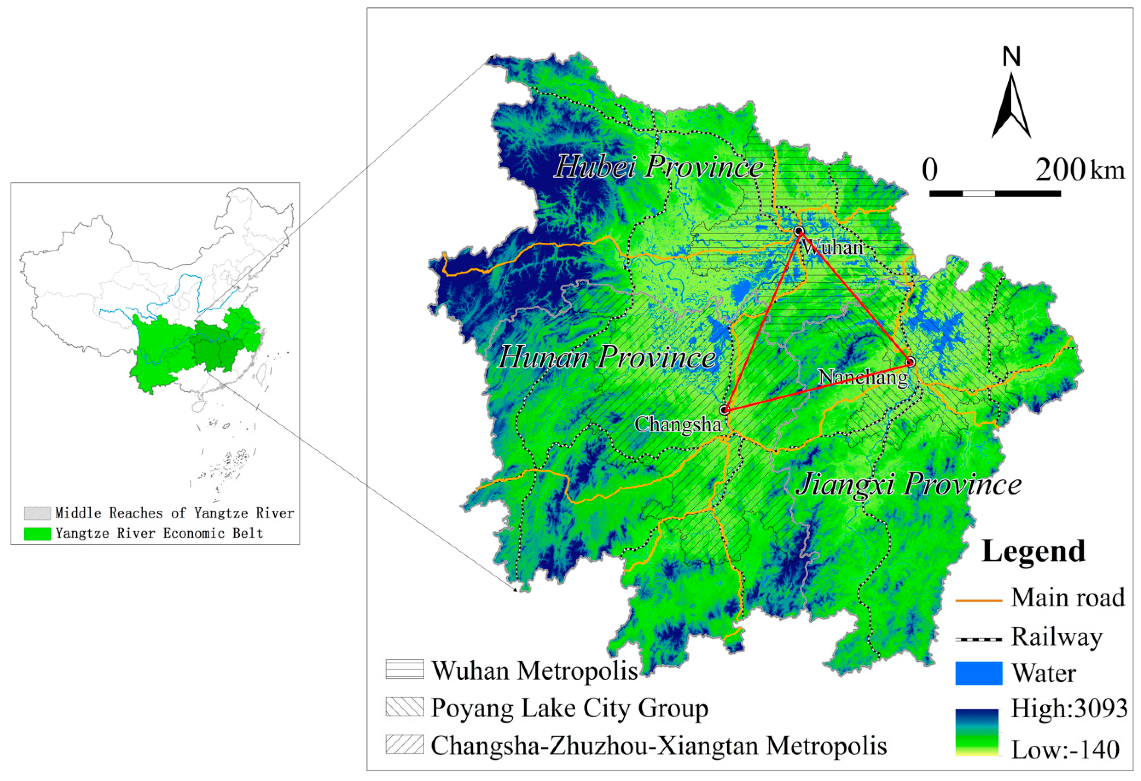
2.1. Study Area and Data

The MRYRUA in this study consists of three provinces: Hunan, Hubei, and Jiangxi (Figure 1). The MRYRUA is located in the transitional zone between China’s second and third steps. The types of landforms in the study area are complex and diverse, with significant spatial differences. The overall terrain is high in the west and low in the north. There are many types of landforms, including plains, hills, and mountains in the MRYRUA. The MRYRUA is surrounded by the Wu Mountains and Xuefeng Mountains in the west, Nanling Mountains in the south, and Wuyi Mountains in the east. The area is rich in farmland, forestland, water resources, and biodiversity, all of which play an important role in grain-producing and ecosystem services provisioning in China. With the Wuhan megalopolis, Changsha–Zhuzou–Xiangtan urban agglomerations, and Poyang Lake city group as its development centers, the MRYRUA has become an emerging national-level urban agglomeration in China. Rapid development in the MRYRUA greatly promoted the land-use transition and the deterioration of ecosystem services. During the period of 1995–2015, deforestation, afforestation, land reclamation, and returning sloping farmland to forestland occurred frequently in the MRYRUA, causing a dramatic effect on regional ecosystem services. In the context of the important strategic position of the MRYRUA and the environmental problems, it is necessary to study the supply capacity of the ecosystem services and their driving mechanism.
The 30-m resolution LULCC dataset was downloaded from the Data Center for Resources and Environmental Sciences, Chinese Academy of Sciences (RESDC) (http://www.resdc.cn) [39]. Landsat TM/ETM+ remote sensing imagery was the primary source of data for the LULCC dataset. Using the human–computer interactive interpretation method, Liu et al. constructed the national LULCC dataset in China at 5-year intervals [39]. According to specific research needs, the land uses are divided into six first-level types—farmland, forestland, grassland, water area, construction land, and unused land. To ensure the quality of the LULCC datasets, nationwide field surveys were conducted; the overall accuracy was over 90% [39,40,41].

2.2. Dependent Variables

The theoretical framework for the measurement of ecosystem services value (ESV) proposed by Costanza et al. (1997) has greatly promoted the study of the assessment of ESV globally [8]. Xie et al. (2003, 2008) revised the ecosystem services classification and equivalent table based on the expertise of ≥700 ecologists in China using the method of Costanza et al. (1997) [42,43]. Specifically, ecosystem services were reclassified into four main types and nine subtypes. The equivalent table of ESV was modified with the concept of equivalent value per unit area. The economic value of grain production per unit area of farmland was assumed to be 1. The equivalent value per unit area of other ecosystem services was identified based on their relative importance to grain production of farmland. The ESV equivalent factor per unit area was defined as equal to 1/7 of the average economic value of grain production per unit area of farmland. Chen et al. (2019a) calculated the ESV equivalent value ($US344.927/(hm2 a)) based on the grain yield data and the grain price data in the MRYRUA [44] (Equation (1)). Ecosystem services have been localized based on biomass, but biomass was not completely positively correlated, particularly in the water areas and wetlands [42]. However, the water area and wetlands in the MRYRUA are vast, contributing more than 10% of the total ESV [44] Chen et al. (2019b) further revised the ESV equivalent value based on the biomass of farmland (Equation (2)). [45] Based on the results of Chen et al. (2019b) [45], we took the average ESV of each county as the dependent variable in 1995, 2005, and 2015. The equations are as follows:
E V = 1 7 × h r × p r × q r M
E S V c o r r e c t e d = V C I k V C I ¯ × j = 1 m i = 1 n ( L U C i × E V i j )
where EV is the economic value of grain production per unit area of farmland (ESV equivalent value; dollars/(hm2· a)); hr is the sown area of the rth grain crop (hm2); pr is the average price of the rth grain crop ($/ton); qr is the per unit area yield of the rth grain crop (ton/hm2); M is the sown area of all the grain crops (hm2); and ESVcorrected indicates the corrected ESV.
VCI indicates the average vegetation condition index computed from the normalized difference vegetation index of the farmland; V C I ¯ indicates the annual average VCI; VCIk is the average VCI of the kth county; EVij is the jth category of ESV equivalent value for the ith land use type; and LUCi represents the area of the ith land-use type.

2.2.1. LULCC in the MRYRUA from 1995 to 2015

Forestland in the MRYRUA accounted for the largest proportion of the total coverage (more than 58%), followed by farmland (30%). Land use in the MRYRUA changed significantly during 1995–2015. Forestland increased slightly from 1995–2005 (0.19%), while a significant decline was witnessed during 2005–2015 (0.60%). The area of farmland showed a continuous downward trend (−0.24% during 1995–2005 and −0.79% during 2005–2015). However, a continuous increase can be found in construction land (0.09% during 1995–2005 and 1.12% during 2005–2015) and water areas (0.26% during 1995–2005 and 0.21% during 2005–2015) (Table 1). Several important trends and transitions between different land-use types are also worth noting during 1995–2015. The most significant transitions happen between farmland and forestland: 5906.48 km2 of forestland converted to farmland, and 5459.57 km2 of farmland converted to forestland. For farmland and construction land, 5001.00 km2 of farmland were converted to construction land, while only 781.48 km2 of construction land were converted to farmland (Table 2). A significant imbalance can be found in the amount of cultivated land transferred in and transferred out during 1995–2005 and 2005–2015. The possible reason is that rapid urbanization took over a large amount of farmland, resulting in a rapid decline in the proportion of farmland. Additionally, since the implementation of the Farmland Balance Policy, the same amount of farmland should be reclaimed to make up for the farmland occupied by construction land, resulting in a large amount of forestland being converted to farmland. At the same time, due to the policy of returning farmland to forestland and the implementation of a series of ecological engineering projects, a large amount of farmland was converted into forestland during the study period.

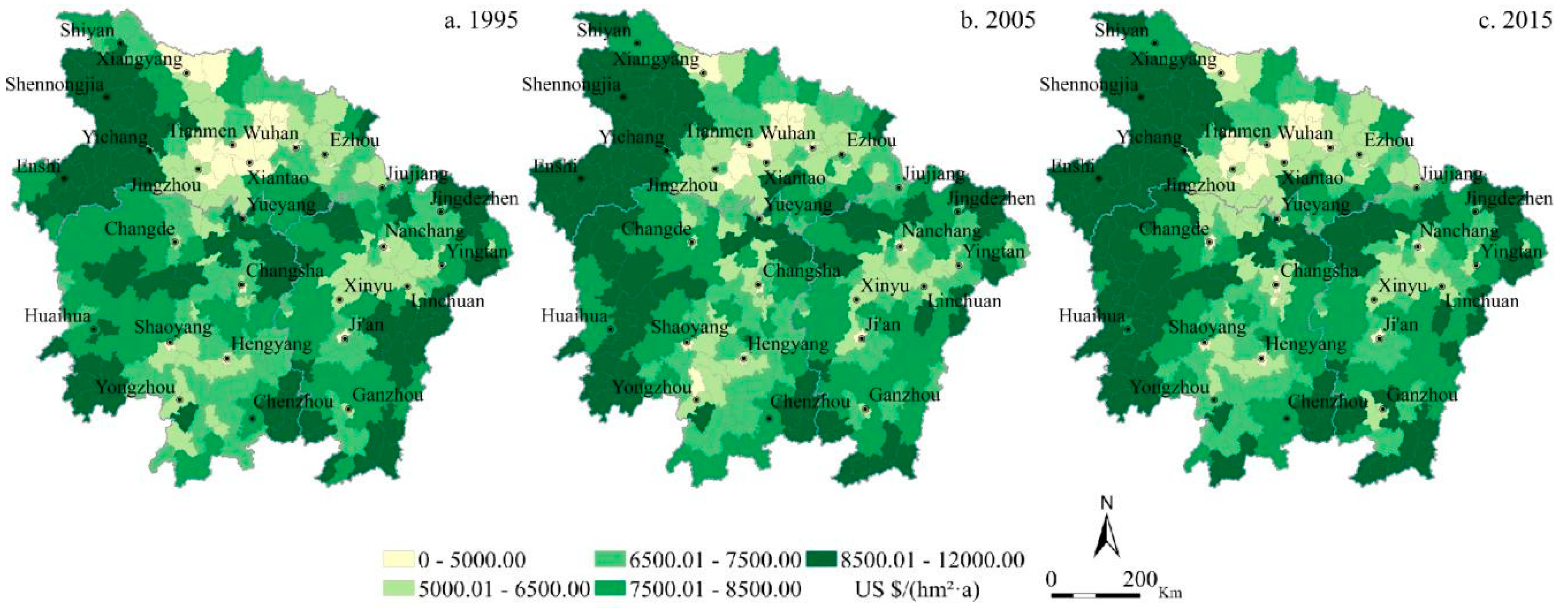
2.2.2. ESV in the MRYRUA from 1995 to 2015

The average ESVs in the MRYRUA in 1995, 2005, and 2015 were US$7724.03/hm2 · a, US$7817.47/hm2 · a, and US$7877.02/hm2 · a, respectively, documenting a gradually increasing trend during the period studied. Forestland provided more than 75% of the ESV in the MRYRUA, while farmland and water areas provided more than 10% of the total ESV (Table 3). The other land-use types, including grassland and unused land, provided only a small proportion of ESV. Among all the ecosystem functions, the hydrological regulation function accounted for the largest proportion of the total ESV (15.79% in 1995, 15.91% in 2005, and 15.98% in 2015). During 1995–2005, the 9 categories of ecosystem functions provided by grassland and unused land decreased, while the ecosystem functions provided by farmland, forestland, and water areas increased. The hydrological regulation function provided by water areas increased the most (US$1101.73 million), while the soil formation and retention function provided by grassland decreased the most (−US$122.97 million). During 2005–2015, only the ecosystem functions provided by farmland decreased. The soil formation and retention function provided by farmland decreased the most significantly (−US$228.37 million). The hydrological regulation function provided by grassland increased the most (US$528.70) during 2005–2015.
In terms of spatial distribution, the spatial pattern of the average ESV in the MRYRUA is relatively stable, and the low-value areas of the average ESV are distributed primarily in the Jianghan Plain, the Poyang Lake Plain, and the Dongting Lake Plain, especially in the key cities and surrounding areas (Figure 2). The high-value areas of the average ESV are mainly south of the Dabie Mountains and Wushan in the western area of Hubei, the Xuefeng Mountains in the central and western part of Hunan Province and Nanling in the southern part of Hunan Province, the Wuyi Mountains in the eastern region of Jiangxi Province, and the Luoxiao Mountains between Jiangxi Province and Hunan Province. The supply capacity of ESV provided by ecosystems varied significantly due to the significant differences in natural conditions and socioeconomic development levels in mountainous and plain areas.

2.3. Independent Variables

Based on the driving factors found in previous studies that impact ecosystem services, for this study we selected population density, road density, and proximity to represent human factors, and selected elevation, slope, temperature, precipitation, and river density to represent physical factors [16,17,18,46]. The proportion of forestland and the proportion of developed land were chosen to represent the land-use pressure [28]. Because a large number of variables may lead to a multicollinearity problem, a variance inflation factor (VIF) test was performed on the independent variables. After the VIF test, a set of factors was selected as independent variables (Table 4).

2.4. Regression Analysis

2.4.1. Spatial Correlation Analysis

The spatial interaction and spatial diffusion assume that the attributes at one location are interdependent with those at other locations [47]. Global spatial autocorrelation and local spatial autocorrelation are commonly used to measure their spatial relationships. The regional spatial dependence of the average ESV was measured with the global Moran’s I index and local Moran’s I Index (LISA). Specifically, global spatial autocorrelation was used to verify the overall aggregation of the specific phenomena or attribute values in the spatial distribution of the entire region, while the local Moran’s I was used to measure the degree of spatial difference between a certain area and its surrounding areas. The scatter plot of Moran’s I provided a clear spatial clustering pattern of average ESV. The first and third quadrants in the scatter plot were, respectively, the high–high and low–low types; and the second and fourth quadrants were, respectively, the low–high and high–low types. The LISA map helps in understanding whether any of the spatial patterns are significant. Based on the statistical hypothesis testing, the Zscore ≥ 1.96 or Zscore ≤ –1.96 showed that the spatial autocorrelation was statistically significant at the 5% level. GeoDa095i software (University of Chicago, Chicago, IL, USA) was employed in this study to test the spatial autocorrelation of the county-level average ESV in the MRYRUA in the years 1995, 2005, and 2015 using the queen’s contiguity weight method [48]. The equations are as follows:
I = n i = 1 n j = 1 n W i j × i = 1 n j = 1 n W i j ( A E S V i A E S V ¯ ) ( A E S V j A E S V ¯ ) i = 1 n ( A E S V i A E S V ¯ ) 2
Z ( I ) = I E ( I ) V a r ( I )
I i = n ( A E S V i A E S V ¯ ) j = 1 n W i j ( A E S V j A E S V ¯ ) i = 1 n ( A E S V i A E S V ¯ ) 2
where AESVi, AESVj are the spatial observations in position i and j, respectively; A E S V ¯ is the average value of ecosystem services; and Wij is the spatial weight connection matrix (i, j = 1,2,3 ... n). E(I) and Var(I) are, respectively, the expected value and the variance of Moran’s I. The global Moran’s I value generally ranged from –1 to 1. Moran’s I values > 0 indicate positive spatial autocorrelation, Moran’s I values < 0 indicate negative spatial autocorrelation, and Moran’s I approaching 0 indicates a random distribution pattern.

2.4.2. Spatial Regression Analysis

The spatial effects of the independent variables have often been neglected in previous research about ecosystem services, and it is commonly assumed that the effects are spatially independent and identically distributed. Using an ordinary least squares (OLS) model (Equation (4)) may lead to an incomplete explanation of the regression results because it ignores the potential spatial effects [49,50]. In this study, we use three spatial regression models, including the spatial lag model (SLM) (Equation (5)), spatial error model (SEM) (Equation (6)), and spatial error model with lag dependence (SEMLD) (Equation (7)) [37,50]. The SLM assumes spatial autocorrelation occurs in the dependent variable, emphasizes the neighborhood effect, and considers the phenomenon of spatial diffusion (the spillover effect) in the dependent variable across geographic units [51]. The SEM focuses on the neglected and unobserved spatial interdependencies among variables. The SEMLD is a spatial autoregressive model augmented by adding the spatially lagged dependent variable to the SEM. All the models were conducted in GeoDa095i at the county level. We identified the performance of the four models based on the log-likelihood value, the Akaike information criterion (AIC), and the Schwarz criterion (SC). The equations are given in Equations (6) through (9):
A E S V t = X t β + ε
A E S V t = X t β + ρ W 1 A E S V t + ε
A E S V t = X t β + ε , ε = λ W 2 ε + ξ
A E S V t = X t β + ρ W 1 A E S V t + ε , ε = λ W 2 ε + ξ
where AESVt is the matrix of dependent variable in time t; Xt is an n × k independent variables matrix in year t; n is the number of study units; k is the number of independent variables; β is a vector of coefficients of Xt indicating the influence level of the independent variables on the dependent variables; ρ is a spatial lag parameter; ε is a random error term vector; λ is a spatial error parameter; and W1 and W2 are spatial weight matrices for the lag term and the error term, respectively.

3. Results

3.1. Spatial Autocorrelation

The exploratory spatial data analysis method was used to further study the spatial distribution of aggregation and abnormalities of average ESV and the relationship of average ESV with the adjacent areas in the MRYRUA. Geoda950i software was used to calculate the Moran’s I of the average ESV from 1995 to 2015 in the MRYRUA. The global Moran’s I analysis of the average ESV indicated that the positive global Moran’s I of the average ESV (0.539 in 1995, 0.576 in 2005, and 0.591 in 2015) in the MRYRUA showed that counties with a high or low average ESV in the MRYRUA exhibited a significant agglomeration distribution pattern. Moreover, the gradual increasing trend of global Moran’s I from 1995 to 2015 indicated that the agglomeration tendency in the MRYRUA was strengthened. Additionally, the observed values of global Moran’s I and expected values (E(I)) did not change significantly, and p was significant at 0.01%, indicating that the average ESV in the MRYRUA remained stable in magnitude and in spatial distribution pattern. The counties of high–high type were concentrated primarily in the mountainous areas (i.e., Wu Mountains in western Hubei, Xuefeng Mountains in western Hunan). The low–low type was distributed chiefly in the central areas of the Wuhan metropolis, Changsha–Zhuzhou–Xiangtan Metropolis, and Poyang Lake city group, which are surrounding counties of major cities. The distribution of the high–low type was apparent in the counties surrounding Nanchang, there were few low–high types distributed discretely during the study period, and the overall LISA clustering pattern of average ESV did not change significantly during the study period (Figure 3).

3.2. Spatial Regression

The Moran’s I analysis indicates that spatial regression models for spatial estimation and verification should be established. After OLS estimation, a Moran’s I index residual test was performed on the residuals; the Moran’s I coefficients in 1995, 2005, and 2015 were 0.400, 0.426, and 0.398, respectively. The p-value was 0.001, indicating strong spatial autocorrelation among the residuals. The spatial dependence diagnostics by the OLS model further showed that statistically significant spatial lag and spatial error terms existed in the model residuals (Table 5). The OLS estimation in the classical linear regression model may have errors in model design with no consideration of spatial autocorrelation. Based on the measures of model fit to the data—AIC, SC, and log-likelihood (Table 5 and Table 6)—the performance of the spatial regression models was better fitted to the data than that of the OLS model. Among the three spatial regression models, the SEMLD had the best fit to the data, with the lowest AIC and SC values and highest log-likelihood.
The regression results of the SEMLD are shown in Table 6. It was unanticipated that population density was insignificant in all the models from 1995 to 2015. The possible reason is that other determinants, such as the proportion of developed land, have advantages over population density, and the impacts of population density were not obvious during these periods. Similar results can be found in Hu et al. (2015) [28]. There was a negative spatial association between road density and ecosystem services, but not in all models. Different levels of road density had different impacts on ecosystem services. Similar results can be found in other studies—i.e., that an increase in the density of roads is associated with a decrease in ecosystem services by leading to landscape fragmentation and strengthening socioeconomic activities [52,53].
Distance to a socioeconomic center proved to be an important spatial determinant for ecosystem services, and there was a positive relationship between ecosystem services and distance to a socioeconomic center. Elevation exhibited a significant positive association with ecosystem services in the years studied, indicating that counties at higher elevation tend to have higher ecosystem services. An increase of 100 m in elevation led to an increase of average ESV by 0.200, 0.136, and 0.148 in SEMLD in 1995, 2005, and 2015, respectively. Precipitation proved statistically significant only in OLS models in 1995 and 2015; the positive relationship suggests that the increase in precipitation promoted the increase of ecosystem services.
River density and ecosystem services were negatively associated in the OLS and SLM models. Numerous studies have provided important evidence that settlements tend to be formed closer to water bodies or rivers [54,55], which inevitably damages the ecosystem. In an additional Pearson’s correlation analysis of river density and construction land, a significant negative correlation was observed in the MRYRUA from 1995 to 2015 (r = 0.111 and p = 0.05 in 1995, r = 0.125 and p = 0.05 in 2005, and r = 0.115 and p = 0.05 in 2015). The proportion of developed land was negatively associated with ecosystem services in all models in 1995, 2005, and 2015. A 1% increase in the proportion of developed land contributed to decreases of 0.497%, 0.402%, and 0.566% in ecosystem services in SEMLD in 1995, 2005, and 2015, respectively. The negative association between the proportion of developed land and ecosystem services indicates that counties with a higher proportion of developed land tended to have lower ecosystem services. An increase in the proportion of developed land means an increase in the consumption of ecosystem services related to human activities, and the literature has shown that an increase in the proportion of developed land leads to ecosystem deterioration [28,56,57]. A statistically significant positive association can be observed between the percentage of forestland and ecosystem services. Using SEMLD for interpretation, 1% of the percentage of forestland increase corresponds to a 0.410%, 0.340%, and 0.319% increase of average ESV, in 1995, 2005, and 2015, respectively.
Spatial lag terms in the SEMLD were statistically significant in 1995, 2005, and 2015, indicating that the spatial spillover effect of ecosystem services was common in the MRYRUA. The ecosystem services in one county were not only closely related to the individual elements (physical and social factors) but also to other neighborhood factors (ecosystem services in adjacent counties). Each 1% increase in average ESV in a neighboring county correlated to 0.276%, 0.134%, and 0.121% increases in each county in 1995, 2005, and 2015, respectively. Moreover, the spatial error terms in the SEMLD were statistically significant in 1995, 2005, and 2015, documenting that ecosystem services were impacted not only by the driving forces studied in this study but were also influenced by other, omitted variables.

4. Discussion and Implications

4.1. A Summary of the Findings

National strategies like the Central China Rising Strategy, the Yangtze River Economic Belt Strategy, and the Triangle of Central China Strategy have greatly promoted urbanization and industrialization in the MRYRUA. As a consequence, a considerable amount of farmland has been converted into construction land. In response, a series of land-use policies, such as the Basic Farmland Protection Regulation, the Farmland Balance Policy, and the increasing versus decreasing balance policy, have been implemented in an attempt to control urban expansion and prevent the decline of farmland [58,59]. However, because of the huge economic benefits gap between farmland and construction land, the targets for construction land expansion control and farmland protection were not met [60]. Additionally, land-use activities, such as deforestation and cultivation, as well as forestry engineering in the shelterbelt program in the upper and middle reaches of the Yangtze River basin, resulted in frequent conversion between farmland and forestland.
Spatial determinants identified in this study further showed negative associations among ecosystem services and road density, the proportion of developed land, and river density, while the distance to a socioeconomic center, proportion of forestland land, elevation, and precipitation were positively associated with ecosystem services. Previous studies have evidenced that developed land tends to expand along road networks [38]. The road network affects the flow of elements and resources within and among regions, and the circulation and accumulation of labor, capital, technology factors, and resources affect population redistribution and land development, directly or indirectly. The geographic characteristic (such as distance to a socioeconomic center) has an evident impact on land-use change [61]. The availability and accessibility of multiple resources in urban centers exacerbate the agglomeration of socioeconomic activities. Ecosystem services around the central counties of cities and surrounding counties are becoming increasingly important. Previous studies provide empirical evidence that human settlements are more likely distributed near water bodies because of invaluable natural amenities [55]. River density is therefore negatively associated with ecosystem services. The positive association between the proportion of forestland and ecosystem services shows that an increase in forestland promotes an increase in ecosystem services. Reforestation is an effective means for improving ecosystem services [28]. The ecosystem services in the MRYRUA display significant spatial autocorrelation and spillover effects, indicating that the ecological conservation and land-use policies in a single area cannot completely solve the problem of regional ecological issues and land-use problems. The prevention and control of ecological issues needs effective coordination across counties, especially in urban agglomerations.

4.2. Policy Implications

In practice, there always exist conflicts among various plans (e.g., economic and social development planning, environmental protection planning, and land-use planning). For example, land-use planning tends to ignore ecological impacts. In response, multiple planning integration efforts have been promoted in China to balance the differences among various spatial plans and avoid unfavorable outcomes. For example, the three designation zones (agricultural, ecological, and urban) and three lines (urban development boundary, ecological red line, and permanent basic farmland red line) are to alleviate the issues of the decline of farmland and the deterioration of ecosystem services due to the expansion of construction land [62]. Therefore, it is necessary to strategically optimize national spatial planning and ecosystem services management. Empirical research shows that the evolution of regional ecosystem services is impacted not only by physical and human factors but also by the charateristics of the neighboring areas. It is noteworthy that ecosystem services in the MRYRUA exhibit significant spatial autocorrelation and spatial spillover features. In other words, regional ecosystem services are affected by ecological regulation and industrial structure as well as by neighboring counties and more distant counties; the ecological conservation regulation policy for a single area cannot completely solve the problem of regional ecological issues [10]. The effective control of ecological issues requires intercounty joint efforts.

4.3. Limitations and Future Research Directions

The revised benefit transfer method and an integrated spatial regression were used to measure the spatial features and the influence mechanism of ecosystem services. However, this study focused only on the supply capacity of the ecosystem services; their demand capacity was an essential aspect of ecosystem services that also should be considered [9]. The study examined only the impact mechanism of total ESV; future research could pay attention to the driving forces of regulating services, supplying services, supporting services, and cultural services. Furthermore, an integrated cross-sectional spatial regression approach was used to identify the spatial determinants of ecosystem services; dynamic spatial panel data models that blend the inter-individual differences and intra-individual dynamics could be considered in future research [63].

5. Conclusions

In this study, we examined the spatiotemporal pattern of the ESV in the MRYRUA from 1995 to 2015 using a revised benefit transfer method. Then we identified the spatial autocorrelation of ESV with the global Moran’s I index and local Moran’s I index. We ultimately analyzed the spatial determinants of average ESV using an integrated spatial regression approach and found a gradually increasing trend in ESV. Forestland provided the greatest proportion of ESV (more than 75%) in the MRYRUA, and farmland and water areas provided more than 10% of the total ESV. The hydrological regulation function accounted for the largest proportion of the total ESV (more than 15%) among all the ecosystem functions. We observed evident spatial dependence and spatial spillover effects of average ESV in the MRYRUA from 1995 to 2015. The average ESV in an area was impacted not only by its factors but also by the characteristics of its neighboring areas due to the spatial spillover effects. The spatial regression results showed that road density, river density, and proportion of developed land were negatively associated with the average ESV, while elevation and precipitation were positively associated with the average ESV. Distance to a socioeconomic center was also found to be an important spatial determinant for average ESV. The results in this study provided important implications for the cross-regional collaborative management of ecosystem services and sustainable land use.

Author Contributions

Conceptualization, W.C. and G.C.; methodology, G.C.; software, W.C.; validation, W.C., G.C., and J.L.; formal analysis, W.C.; investigation, W.C.; resources, J.L.; data curation, W.C.; writing—original draft preparation, W.C.; writing—review and editing, G.C.; visualization, W.C.; supervision, G.C.; project administration, J.L. All authors have read and agreed to the published version of the manuscript.

Funding

The research is sponsored in part by the Natural Science Foundation of China (Grant No. 41701629) and support from the Open Topic of Hunan Key Laboratory of Land Resources Evaluation and Utilization (Grant No. SYS-MT-201903).

Acknowledgments

The authors also would like to thank the anonymous reviewers for their constructive comments on improving this paper.

Conflicts of Interest

The authors declare no conflict of interest.

References

  1. Fang, C.; Cui, X.; Li, G.; Bao, C.; Wang, Z.; Ma, H.; Sun, S.; Liu, H.; Luo, K.; Ren, Y. Modeling regional sustainable development scenarios using the urbanization and eco-environment coupler: Case study of Beijing-Tianjin-Hebei urban agglomeration, China. Sci. Total Environ. 2018, 689, 820–830. [Google Scholar] [CrossRef] [PubMed]
  2. Wang, C.; Li, X.; Yu, H.; Wang, Y. Tracing the spatial variation and value change of ecosystem services in Yellow River Delta, China. Ecol. Indic. 2019, 96, 270–277. [Google Scholar] [CrossRef]
  3. Long, H.; Liu, Y.; Hou, X.; Li, T.; Li, Y. Effects of land use transitions due to rapid urbanization on ecosystem services: Implications for urban planning in the new developing area of China. Habitat Int. 2014, 44, 536–544. [Google Scholar] [CrossRef]
  4. National Development and Reform Commission (NDRC). The Yangtze River Middle Reach City Group Development Plan. 2015. Available online: https://www.ndrc.gov.cn/xxgk/zcfb/tz/201504/t20150416_963800.html (accessed on 4 February 2020).
  5. Ehrlich, P.R.; Ehrlich, A.H. Extinction: The Causes and Consequences of the Disappearance of Species; RandomHouse: New York, NY, USA, 1981. [Google Scholar]
  6. Carroll, M.; Wilson, W.H.M. Man’s Impact on the Global Environment; MIT Press: Cambridge, UK, 1970. [Google Scholar]
  7. Westman, W.E. How much are nature’s services worth? Science 1977, 197, 960–964. [Google Scholar] [CrossRef] [PubMed]
  8. Costanza, R.; DArge, R.; DeGroot, R.; Farber, S.; Grasso, M.; Hannon, B.; Limburg, K.; Naeem, S.; ONeill, R.V.; Paruelo, J.; et al. The value of the world’s ecosystem services and natural capital. Nature 1997, 378, 253–260. [Google Scholar] [CrossRef]
  9. Chen, W.; Chi, G.; Li, J. The spatial aspect of ecosystem services balance and its determinants. Land Use Policy 2020, 90, 104263. [Google Scholar] [CrossRef]
  10. Chen, W.; Chi, G.; Li, J. The spatial association of ecosystem services with land use and land cover change at the county level in China, 1995–2015. Sci. Total Environ. 2019, 669, 459–470. [Google Scholar] [CrossRef]
  11. Schröter, M.; Koellner, T.; Alkemade, R.; Arnhold, S.; Bagstad, K.J.; Erb, K.; Frank, K.; Kastner, T.; Kissinger, M.; Liu, J.; et al. Interregional flows of ecosystem services: Concepts, typology and four cases. Ecosyst. Serv. 2018, 31, 231–241. [Google Scholar] [CrossRef]
  12. Nelson, E.; Mendoza, G.; Regetz, J.; Polasky, S.; Tallis, H.; Cameron, D.R.; Chan, K.M.A.; Daily, G.C.; Goldstein, J.; Kareiva, P.M.; et al. Modeling multiple ecosystem services, biodiversity conservation, commodity production, and tradeoffs at landscape scales. Front. Ecol. Environ. 2009, 7, 4–11. [Google Scholar] [CrossRef]
  13. Costanza, R.; de Groot, R.; Braat, L.; Kubiszewski, I.; Fioramonti, L.; Sutton, P.; Farber, S.; Grasso, M. Twenty years of ecosystem services: How far have we come and how far do we still need to go? Ecosyst. Serv. 2017, 28, 1–16. [Google Scholar] [CrossRef]
  14. Chi, G.; Marcouiller, D.W. Natural amenities and their effects on migration along the urban-rural continuum. Ann. Reg. Sci. 2013, 50, 861–883. [Google Scholar] [CrossRef]
  15. Li, G.; Fang, C.; Wang, S. Exploring spatiotemporal changes in ecosystem-service values and hotspots in China. Sci. Total Environ. 2016, 545–546, 609–620. [Google Scholar] [CrossRef] [PubMed]
  16. Chen, M.; Lu, Y.; Ling, L.; Wan, Y.; Luo, Z.; Huang, H. Drivers of changes in ecosystem service values in Ganjiang upstream watershed. Land Use Policy 2015, 47, 247–252. [Google Scholar] [CrossRef]
  17. Wu, X.; Liu, S.; Zhao, S.; Hou, X.; Xu, J.; Dong, S.; Liu, G. Quantification and driving force analysis of ecosystem services supply, demand and balance in China. Sci. Total Environ. 2019, 652, 1375–1386. [Google Scholar] [CrossRef] [PubMed]
  18. Zhang, Z.; Gao, J.; Fan, X.; Lan, Y.; Zhao, M. Response of ecosystem services to socioeconomic development in the Yangtze River Basin, China. Ecol. Indic. 2017, 72, 481–493. [Google Scholar] [CrossRef]
  19. Ouyang, Z.; Zheng, H.; Xiao, Y.; Polasky, S.; Liu, J.; Xu, W.; Wang, Q.; Zhang, L.; Xiao, Y.; Rao, E.; et al. Improvements in ecosystem services from investments in natural capital. Science 2016, 352, 1455–1459. [Google Scholar] [CrossRef]
  20. Zhang, L.; Lü, Y.; Fu, B.; Dong, Z.; Zeng, Y.; Wu, B. Mapping ecosystem services for China’s ecoregions with a biophysical surrogate approach. Landsc. Urban Plan. 2017, 161, 22–31. [Google Scholar] [CrossRef]
  21. Wang, Y.; Dai, E.; Yin, L.; Ma, L. Land use/land cover change and the effects on ecosystem services in the Hengduan Mountain region, China. Ecosyst. Serv. 2018, 34, 55–67. [Google Scholar] [CrossRef]
  22. Locatelli, B.; Lavorel, S.; Sloan, S.; Tappeiner, U.; Geneletti, D. Characteristic trajectories of ecosystem services in mountains. Front. Ecol. Environ. 2017, 15, 150–159. [Google Scholar] [CrossRef]
  23. Sil, Â.; Rodrigues, A.P.; Carvalho-Santos, C.; Nunes, J.P.; Honrado, J.; Alonso, J.; Marta-Pedroso, C.; Azevedo, J.C. Trade-offs and synergies between provisioning and regulating ecosystem services in a mountain area in Portugal affected by landscape change. Mt. Res. Dev. 2016, 36, 452–464. [Google Scholar] [CrossRef] [Green Version]
  24. Messerli, B.; Grosjean, M.; Hofer, T.; Núñezc, L.; Pfisterd, C. From nature-dominated to human-dominated environmental changes. Quat. Sci. Rev. 2000, 19, 459–479. [Google Scholar] [CrossRef]
  25. Kertész, Á.; Nagy, L.A.; Balázs, B. Effect of land use change on ecosystem services in Lake Balaton Catchment. Land Use Policy 2019, 80, 430–438. [Google Scholar] [CrossRef]
  26. Cao, S.; Chen, L.; Shankman, D.; Wang, C.; Wang, X.; Zhang, H. Excessive reliance on afforestation in China’s arid and semi-arid regions: Lessons in ecological restoration. Earth Sci. Rev. 2011, 104, 240–245. [Google Scholar] [CrossRef]
  27. Chazdon, R.L. Beyond deforestation: Restoring forests and ecosystem services on degraded lands. Science 2008, 320, 1458–1460. [Google Scholar] [CrossRef] [PubMed] [Green Version]
  28. Miao, Z.; Marrs, R. Ecological restoration and land reclamation in open-cast mines in Shanxi Province, China. J. Environ. Manag. 2000, 59, 205–215. [Google Scholar] [CrossRef]
  29. Buyantuyev, A.; Wu, J. Urbanization alters spatiotemporal patterns of ecosystem primary production: A case study of the Phoenix metropolitan region, USA. J. Arid Environ. 2009, 73, 512–520. [Google Scholar] [CrossRef]
  30. Zhang, Y.; Liu, Y.; Zhang, Y.; Liu, Y.; Zhang, G.; Chen, Y. On the spatial relationship between ecosystem services and urbanization: A case study in Wuhan, China. Sci. Total Environ. 2018, 637–638, 780–790. [Google Scholar] [CrossRef] [PubMed]
  31. Black, R.; Adger, W.N.; Arnell, N.W.; Dercon, S.; Geddes, A.; Thomas, D. The effect of environmental change on human migration. Glob. Environ. Chang. 2011, 21, S3–S11. [Google Scholar] [CrossRef]
  32. Hu, X.; Hong, W.; Qiu, R.; Hong, T.; Chen, C.; Wu, C. Geographic variations of ecosystem service intensity in Fuzhou City, China. Sci. Total Environ. 2015, 512–513, 215–226. [Google Scholar] [CrossRef]
  33. Spellerberg, I. Ecological effects of roads and traffic: A literature review. Glob. Eco. Biogeogr. Lett. 1998, 7, 317–333. [Google Scholar] [CrossRef]
  34. Xu, W.; Xiao, Y.; Zhang, J.; Yang, W.; Zhang, L.; Hull, V.; Wang, Z.; Zheng, H.; Liu, J.; Polasky, S.; et al. Strengthening protected areas for biodiversity and ecosystem services in China. Proc. Natl. Acad. Sci. USA 2017, 114, 1601–1606. [Google Scholar] [CrossRef] [PubMed] [Green Version]
  35. Peng, J.; Tian, L.; Liu, Y.; Zhao, M.; Hu, Y.; Wu, J. Ecosystem services response to urbanization in metropolitan areas: Thresholds identification. Sci. Total Environ. 2017, 607–608, 706–714. [Google Scholar] [CrossRef] [PubMed]
  36. Wang, J.; Zhou, W.; Pickett, S.T.A.; Yu, W.; Li, W. A multiscale analysis of urbanization effects on ecosystem services supply in an urban megaregion. Sci. Total Environ. 2019, 662, 824–833. [Google Scholar] [CrossRef]
  37. Chi, G. The impacts of highway expansion on population change: An integrated spatial approach. Rural Sociol. 2010, 75, 58–89. [Google Scholar] [CrossRef]
  38. Tan, R.; Liu, Y.; Liu, Y.; He, Q.; Ming, L.; Tang, S. Urban growth and its determinants across the Wuhan urban agglomeration, central China. Habitat Int. 2014, 44, 268–281. [Google Scholar] [CrossRef]
  39. Liu, J.Y.; Kuang, W.; Zhang, Z.; Xu, X.; Qin, Y.; Ning, J.; Zhou, W.; Zhang, S.; Li, R.; Yan, C.; et al. Spatiotemporal characteristics, patterns, and causes of land-use changes in China since the late 1980s. J. Geogr. Sci. 2014, 24, 195–210. [Google Scholar] [CrossRef]
  40. Liu, J.; Liu, M.; Zhuang, D.; Zhang, Z.; Deng, X. Study on spatial pattern of land-use change in China during 1995–2000. Sci. China Ser. D Earth Sci. 2003, 46, 373–384. [Google Scholar]
  41. Ning, J.; Liu, J.; Kuang, W.; Xu, X.; Zhang, S.; Yan, C.; Li, R.; Wu, S.; Hu, Y.; Du, G.; et al. Spatiotemporal patterns and characteristics of land-use change in China during 2010–2015. J. Geogr. Sci. 2018, 28, 547–562. [Google Scholar] [CrossRef] [Green Version]
  42. Xie, G.; Zhen, L.; Lu, C.; Xiao, Y.; Chen, C. Expert knowledge based valuation method of ecosystem services in China. J. Nat. Res. 2008, 23, 911–919. [Google Scholar]
  43. Xie, G.; Lu, C.; Leng, Y.; Zheng, D.; Li, S. Ecological assets valuation of the Tibetan Plateau. J. Nat. Res. 2003, 18, 189–196. [Google Scholar]
  44. Chen, W.; Li, J.; Zhu, L. Spatial heterogeneity and sensitivity analysis of ecosystem services value in the Middle Yangtze River region. J. Nat. Resour. 2019, 34, 325–337. [Google Scholar]
  45. Chen, W.; Zhao, H.; Li, J.; Zhu, L.; Wang, Z.; Zeng, J. Land use transitions and the associated impacts on ecosystem services in the Middle Reaches of the Yangtze River Economic Belt in China based on the geo-informatic Tupu method. Sci. Total Environ. 2019, 701, 134690. [Google Scholar] [CrossRef]
  46. Feng, Q.; Zhao, W.; Fu, B.; Ding, J.; Wang, S. Ecosystem service trade-offs and their influencing factors: A case study in the Loess Plateau of China. Sci. Total Environ. 2017, 607–608, 1250–1263. [Google Scholar] [CrossRef] [PubMed]
  47. Tobler, W.R. A computer movie simulating urban growth in the Detroit Region. Econ. Geogr. 1970, 46, 234–240. [Google Scholar] [CrossRef]
  48. Anselin, L. Local indicators of spatial association—LISA. Geogr. Anal. 1995, 27, 93–115. [Google Scholar] [CrossRef]
  49. Anselin, L. A test for spatial autocorrelation in seemingly unrelated regressions. Econ. Lett. 1988, 28, 335–341. [Google Scholar] [CrossRef]
  50. Chi, G.; Zhu, J. Spatial Regression Models for the Social Sciences; SAGE Publications: Thousand Oaks, CA, USA, 2019. [Google Scholar]
  51. Chi, G.; Zhu, J. Spatial regression models for demographic analysis. Popul. Res. Policy Rev. 2008, 27, 17–42. [Google Scholar] [CrossRef]
  52. Brander, L.M.; Wagtendonk, A.J.; Hussain, S.S.; McVittie, A.; Verburg, P.H.; de Groot, R.S.; van der Ploeg, S. Ecosystem service values for mangroves in Southeast Asia: A meta-analysis and value transfer application. Ecosyst. Serv. 2012, 1, 62–69. [Google Scholar] [CrossRef] [Green Version]
  53. Müller, K.; Steinmeier, C.; Küchler, M. Urban growth along motorways in Switzerland. Landsc. Urban Plan. 2010, 98, 3–12. [Google Scholar] [CrossRef]
  54. Braimoh, A.K.; Onishi, T. Spatial determinants of urban land use change in Lagos, Nigeria. Land Use Policy 2007, 24, 502–515. [Google Scholar] [CrossRef]
  55. Riera, J.; Voss, P.R.; Carpenter, S.R.; Riera, J.; Voss, P.R.; Carpenter, S.R.; Kratz, T.K.; Lillesand, T.M.; Schnaiberg, J.A.; Turner, M.G.; et al. Nature, society and history in two contrasting landscapes in Wisconsin, USA: Interactions between lakes and humans during the twentieth century. Land Use Policy 2001, 18, 41–51. [Google Scholar] [CrossRef]
  56. Wang, J.; Zhai, T.; Lin, Y.; Kong, X.; Ting, H. Spatial imbalance and changes in supply and demand of ecosystem services in China. Sci. Total Environ. 2019, 657, 781–791. [Google Scholar] [CrossRef] [PubMed]
  57. Su, S.; Li, D.; Hu, Y.N.; Xiao, R.; Zhang, Y. Spatially non-stationary response of ecosystem service value changes to urbanization in Shanghai, China. Ecol. Indic. 2014, 45, 332–339. [Google Scholar] [CrossRef]
  58. Lichtenberg, E.; Ding, C. Assessing farmland protection policy in China. Land Use Policy 2008, 25, 59–68. [Google Scholar] [CrossRef]
  59. Chen, W.; Ye, X.; Li, J.; Fan, X.; Liu, Q.; Dong, W. Analyzing requisition–compensation balance of farmland policy in China through telecoupling: A case study in the middle reaches of Yangtze River Urban Agglomerations. Land Use Policy 2019, 83, 134–146. [Google Scholar] [CrossRef]
  60. Shen, X.; Wang, L.; Wu, C.; Lv, T.; Lu, Z.; Luo, W.; Li, G. Local interests or centralized targets? How China’s local government implements the farmland policy of Requisition–Compensation Balance. Land Use Policy 2017, 67, 716–724. [Google Scholar] [CrossRef]
  61. Liu, Y.; Long, H. Land use transitions and their dynamic mechanism: The case of the Huang-Huai-Hai Plain. J. Geogr. Sci. 2016, 26, 515–530. [Google Scholar] [CrossRef] [Green Version]
  62. Lian, X. Review on advanced practice of provincial spatial planning: Case of a western, less developed province. Int. Rev. Spat. Plan. Sustain. Dev. 2018, 6, 185–202. [Google Scholar] [CrossRef] [Green Version]
  63. Hsiao, C. Panel data analysis—Advantages and challenges. Test 2007, 16, 1–22. [Google Scholar] [CrossRef] [Green Version]
Figure 1. Location of the study area in China.
Ijerph 17 03717 g001
Figure 2. The spatial pattern of ecosystem services supply capacity in the MRYRUA from 1995 to 2015. (a) Ecosystem services supply capacity in 1995. (b) Ecosystem services supply capacity in 2005. (c) Ecosystem services supply capacity in 2015.
Ijerph 17 03717 g002
Figure 3. LISA clustering of ecosystem services supply capacity in the MRYRUA from 1995 to 2015. (a) LISA clustering of ecosystem services supply capacity in 1995. (b) LISA clustering of ecosystem services supply capacity in 2005. (c) LISA clustering of ecosystem services supply capacity in 2015.
Ijerph 17 03717 g003
Table 1. Area and changes of land-use types in the Middle Reaches of the Yangtze River Urban Agglomerations (MRYRUA) from 1995 to 2015.
Land Use TypeUnits1995200520151995–20052005–20151995–2015
FarmlandArea (km2)176,032.81174,649.62170,191.07−1383.19−4458.55−5841.74
Proportion (%)31.1730.9330.14−0.24−0.79−1.03
ForestlandArea (km2)330,189.84331,286.12327,894.711096.28−3391.41−2295.13
Proportion (%)58.4758.6758.070.19−0.60−0.41
GrasslandArea (km2)21,920.5120,241.3020,585.03−1679.20343.73−1335.47
Proportion (%)3.883.583.65−0.300.06−0.24
Water areaArea (km2)25,857.5427,360.3028,500.411502.761140.112642.87
Proportion (%)4.584.845.050.260.210.47
Construction landArea (km2)10,575.6911,055.8417,402.33480.156346.486826.64
Proportion (%)1.871.963.080.091.121.21
Unused landArea (km2)95.378.5297.66−16.7819.142.35
Proportion (%)0.020.010.02000
Table 2. Transition matrix of land use from 1995 to 2015 in the MRYRUA.
YearLand Use TypeFarmlandForestlandGrasslandWater AreaConstruction LandUnused Land
1995–2015Farmland161,659.565906.48538.051299.92781.485.58
Forestland5459.57320,176.401814.89297.64137.818.39
Grassland340.46922.6519,248.4457.8213.961.70
Water area3567.13786.77115.7323,919.71109.771.30
Construction land5001.002375.86202.15280.699532.2110.41
Unused land5.0421.271.221.760.4567.93
1995–2005Farmland163,167.327641.20657.951596.111576.5910.45
Forestland7628.76320,480.642467.68465.45233.649.95
Grassland415.38905.0318,681.15221.5216.401.83
Water area3092.75641.9679.6923,421.04124.190.67
Construction land1724.81517.5933.58152.238624.303.33
Unused land3.793.420.471.190.5669.08
2005–2015Farmland159,171.537739.92491.301827.54956.794.17
Forestland7279.17318,331.521509.28531.42238.845.62
Grassland531.492160.8317,828.3544.5019.241.20
Water area2631.06850.68232.8824,640.65144.490.69
Construction land5026.102181.54178.46314.469694.747.05
Unused land10.4222.301.651.751.7459.80
Notes: Rows show land-use types in 2015, and columns show land-use types in 1995. The number 5906.48 indicates 5906.48 km2 of forestland converted to farmland, while the number 5459.57 indicates 5459.57 km2 of farmland converted to forestland during 1995–2015; the other numbers follow the same rule.
Table 3. Ecosystem services value (ESVs) of different land-use types from 1995 to 2015 (million US$).
YearLand Use TypeSupplying ServicesRegulating ServicesSupporting ServicesCultural Services
Food ProductionRaw MaterialGas RegulationClimate RegulationHydrological RegulationWaste TreatmentSoil Formation and RetentionBiodiversity ProtectionRecreation and CultureTotal
1995Farmland6218.562425.244477.366032.004788.298643.809141.286342.931057.1649,126.63
Forestland3908.0235,290.6451,159.5948,198.9648,435.8120,369.0947,606.8453,409.6624,632.39333,011.01
Grassland336.79281.971174.871221.861190.531033.881754.471464.67681.429140.46
Water area398.88264.431308.696996.0914,435.8713,109.261075.633191.044091.8844,871.76
Unused land0.060.130.190.410.220.830.541.270.764.43
2005Farmland6238.382432.974491.636051.234803.558671.349170.416363.141060.5249,283.17
Forestland3935.4435,538.2551,518.5448,537.1448,775.6520,512.0147,940.8653,784.4024,805.22335,347.51
Grassland313.19262.201092.521136.221107.08961.421631.491362.01633.668499.79
Water area429.32284.611408.567530.0215,537.6014,109.741157.723434.584404.1748,296.33
Unused land0.050.110.160.360.190.710.471.090.663.80
2015Farmland6083.022372.384379.785900.534683.938455.408942.046204.681034.1148,055.87
Forestland3965.8635,812.9551,916.7648,912.3249,152.6720,670.5648,311.4354,200.1324,996.96337,939.63
Grassland326.22273.111137.961183.481153.131001.411699.361418.66660.028853.34
Water area443.93294.291456.497786.2416,066.3014,589.851197.123551.454554.0349,939.70
Unused land19.827.7314.2719.2215.2627.5429.1320.213.37156.54
1995–2005Farmland27.42247.61358.95338.18339.84142.92334.02374.74172.832336.51
Forestland−23.61−19.76−82.35−85.64−83.45−72.47−122.97−102.66−47.76−640.67
Grassland30.4420.1899.88533.931101.731000.4882.09243.54312.293424.56
Water area−0.01−0.02−0.03−0.06−0.03−0.12−0.08−0.18−0.11−0.63
Unused land−155.36−60.59−111.86−150.69−119.62−215.94−228.37−158.46−26.41−1227.31
2005–2015Farmland30.42274.70398.22375.18377.02158.55370.57415.73191.742592.12
Forestland13.0310.9145.4447.2646.0539.9967.8656.6526.36353.55
Grassland14.619.6847.93256.22528.70480.1139.39116.87149.861643.37
Water area0.010.030.040.090.050.180.120.270.160.95
Unused land−135.54−52.86−97.59−131.47−104.37−188.40−199.24−138.25−23.04−1070.76
1995–2015Farmland57.84522.31757.17713.35716.86301.47704.59790.47364.564928.63
Forestland−10.58−8.86−36.91−38.38−37.40−32.48−55.11−46.01−21.40−287.12
Grassland45.0529.86147.81790.161630.431480.59121.48360.40462.155067.94
Water area0.000.010.010.030.020.060.040.090.060.33
Unused land19.827.7314.2719.2215.2627.5429.1320.213.37156.54
Table 4. Variable descriptions and data sources.
Variable CategoryVariableDescriptionData Sources
Dependent variableAESVAverage ecosystem services valueCalculated from Section 2.2.2
Physical driving forcesElevation (m)Average elevationGeospatial Data Cloud Site, Computer Network Information Center, Chinese Academy of Sciences (http://www.gscloud.cn)
Precipitation (mm)Annual average precipitationData Center for Resources and Environmental Sciences, Chinese Academy of Sciences (RESDC) (http://www.resdc.cn)
River density (km/km2)River length per square kilometerNational Geomatics Center of China (NGCC) (http://ngcc.sbsm.gov.cn/)
Proportion of developed landTotal developed land divided by the administrative areaExtracted from LULCC data
Proportion of forestland landTotal forestland divided by the administrative areaExtracted from LULCC data
Socioeconomic driving forcesPopulation density (person/km2)Total population divided by the administrative areaData Center for Resources and Environmental Sciences, Chinese Academy of Sciences (RESDC) (http://www.resdc.cn)
Railway density (km/km2)Railway length per square kilometerNational Geomatics Center of China (NGCC) (http://ngcc.sbsm.gov.cn/)
Highway density (km/km2)Highway length per square kilometerNational Geomatics Center of China (NGCC) (http://ngcc.sbsm.gov.cn/)
National road density (km/km2)National road length per square kilometerNational Geomatics Center of China (NGCC) (http://ngcc.sbsm.gov.cn/)
Distance to socioeconomic center (km)Distance to socioeconomic centerCalculated by ArcGIS10.3 software’s Near tool
Table 5. Regression results of the ordinary least squares (OLS), spatial lag model (SLM), and spatial error model (SEM) from 1995 to 2015.
Variable199520052015
OLSSLMSEMOLSSLMSEMOLSSLMSEM
Population density−0.104
(0.094)
−0.086
(0.086)
−0.085
(0.073)
−0.009
(0.098)
0.008
(0.086)
0.020
(0.075)
−0.050
(0.088)
−0.033
(0.080)
−0.001
(0.071)
Railway density−0.063
(0.055)
−0.051
(0.051)
−0.004
(0.042)
−0.174 *
(0.093)
−0.180 **
(0.082)
−0.161 **
(0.066)
−0.012
(0.096)
−0.049
(0.089)
−0.017
(0.067)
Highway density0.006
(0.046)
0.025
(0.042)
−0.030
(0.041)
−0.021
(0.048)
−0.009
(0.042)
−0.006
(0.041)
−0.078 *
(0.041)
−0.087 **
(0.038)
−0.056
(0.035)
National road density−0.076
(0.052)
−0.088 *
(0.048)
−0.022
(0.037)
−0.107 **
(0.054)
−0.126 ***
(0.048)
−0.049
(0.038)
−0.072
(0.058)
−0.097 *
(0.054)
−0.039
(0.043)
Distance to socioeconomic center0.061 **
(0.030)
0.055 **
(0.028)
0.030
(0.035)
0.086 ***
(0.031)
0.075 ***
(0.028)
0.096 ***
(0.035)
0.042
(0.029)
0.043 *
(0.026)
0.075 **
(0.033)
Proportion of developed land−0.383 ***
(0.073)
−0.284 ***
(0.069)
−0.437 ***
(0.057)
−0.367 ***
(0.077)
−0.226 ***
(0.071)
−0.367 ***
(0.061)
−0.558 ***
(0.085)
−0.402 ***
(0.082)
−0.527 ***
(0.067)
Proportion of forestland land0.238 ***
(0.027)
0.185 ***
(0.027)
0.394 ***
(0.031)
0.216 ***
(0.027)
0.164 ***
(0.026)
0.326 ***
(0.031)
0.193 ***
(0.026)
0.158 ***
(0.025)
0.308 ***
(0.030)
Elevation0.124 **
(0.048)
0.059
(0.045)
0.179 ***
(0.059)
0.150 ***
(0.048)
0.055
(0.044)
0.124 **
(0.058)
0.201 ***
(0.044)
0.105 **
(0.043)
0.135 **
(0.055)
Precipitation0.053 **
(0.026)
0.026
(0.024)
0.113
(0.076)
0.004
(0.025)
−0.011
(0.022)
0.020
(0.057)
0.041 *
(0.024)
0.016
(0.022)
0.054
(0.053)
River density−0.132 ***
(0.040)
−0.133 ***
(0.037)
−0.013
(0.028)
−0.089 ***
(0.040)
−0.092 **
(0.035)
−0.001
(0.029)
−0.092 **
(0.037)
−0.095 ***
(0.034)
−0.005
(0.028)
Spatial lag term0.359 ***
(0.058)
0.419 ***
(0.054)
0.334 ***
(0.053)
Spatial error term0.827 ***
(0.034)
0.753 ***
(0.042)
0.742 ***
(0.043)
Constant0.503 ***
(0.025)
0.324 ***
(0.034)
0.345 ***
(0.051)
0.570 ***
(0.026)
0.330 ***
(0.035)
0.462 ***
(0.041)
0.576 ***
(0.023)
0.390 ***
(0.034)
0.468 ***
(0.036)
Moran’s I (error)0.400 ***0.426 ***0.398 ***
LM (lag)47.520 ***67.119 ***43.151 ***
Robust LM (lag)10.205 **2.860 *3.965 *
LM (error)132.710 ***150.926 ***131.176 ***
Robust LM (error)95.395 ***86.667 ***91.989 ***
LM (lag and error)142.915 ***153.786 ***135.141 ***
Measures of fit
Log likelihood341.339360.724415.646339.456367.692409.750367.818386.784431.184
AIC−660.678−697.449−809.292−656.913−711.383−797.501−713.636−749.568−840.368
SC−619.056−652.043−767.670−615.291−665.977−755.878−672.014−704.162−798.746
N325325325325325325325325325
Notes: The study uses the queen’s contiguity weight matrix. *** p ≤ 0.01, ** p ≤ 0.05, * p ≤ 0.1. Standard errors are in parentheses. LM = Lagrange multiplier. AIC = Akaike information criterion. SC = Schwarz criterion.
Table 6. Regression results of the spatial error models with lag dependence from 1995 to 2015.
Variable199520052015
Population density−0.074
(0.071)
0.021
(0.074)
0.002
(0.070)
Railway density−0.014
(0.041)
−0.156 **
(0.065)
−0.006
(0.066)
Highway density−0.041
(0.039)
−0.001
(0.040)
−0.045
(0.035)
National road density0.001
(0.036)
−0.035
(0.038)
−0.025
(0.043)
Distance to socioeconomic center0.047
(0.035)
0.107 ***
(0.036)
0.086 **
(0.034)
Proportion of developed land−0.497 ***
(0.057)
−0.402 ***
(0.063)
−0.566 ***
(0.069)
Proportion of forestland land0.410 ***
(0.030)
0.340 ***
(0.031)
0.319 ***
(0.030)
Elevation0.200 ***
(0.059)
0.136 **
(0.060)
0.148 ***
(0.056)
Precipitation0.096
(0.086)
0.025
(0.063)
0.056
(0.057)
River density0.003
(0.027)
0.008
(0.029)
0.002
(0.027)
Spatial lag term−0.276 ***
(0.071)
−0.134 *
(0.071)
−0.121 *
(0.066)
Spatial error term0.864 ***
(0.029)
0.790 ***
(0.038)
0.774 ***
(0.040)
Constant0.499 ***
(0.073)
0.533 ***
(0.062)
0.533 ***
(0.056)
Measures of fit
Log likelihood422.660411.177432.621
AIC−821.320−798.355−841.242
SC−775.914−752.949−795.836
N325325325
Notes: The study uses the queen’s contiguity weight matrix. *** p ≤ 0.01, ** p ≤ 0.05, * p ≤ 0.1. Standard errors are in parentheses. LM = Lagrange multiplier. AIC = Akaike information criterion. SC = Schwarz criterion.

