Cascading Failures and Vulnerability Evolution in Bus–Metro Complex Bilayer Networks under Rainstorm Weather Conditions


Abstract
1. Introduction
2. The Influence of Rainstorm on Bus–Metro CBN
2.1. The impact of rainstorm on roads and metro train tracks
2.2. The impact of rainstorm on vehicles
2.3. The impact of rainstorm on drivers and passengers
3. Models and Methods
3.1. Constructing the Bus–Metro CBN
3.1.1. Research Hypothesis
3.1.2. Symbolic Description of the Bus–Metro CBN
3.2. Cascading Failure Model of Bus–Metro CBN under Rainstorm Conditions
3.2.1. Passenger Flow Transfer Rules for Cascading Failures in Bus–Metro CBN
3.2.2. Cascading Failure Model based on CMLs
3.3. Vulnerability Analysis of Bus–Metro CBN under Rainstorm
4. Case Study
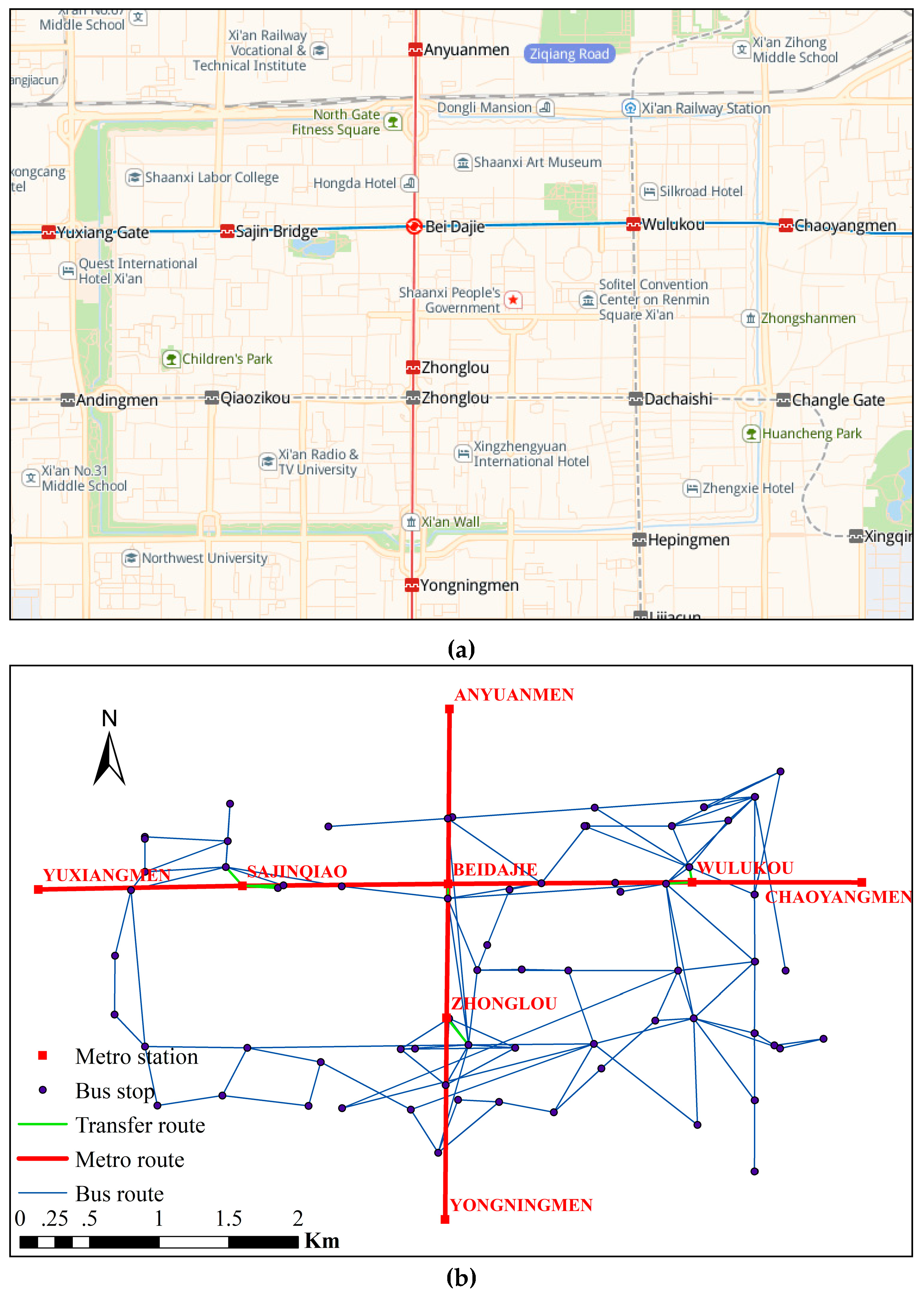
4.1. Research Area
4.2. Scenario Descriptions
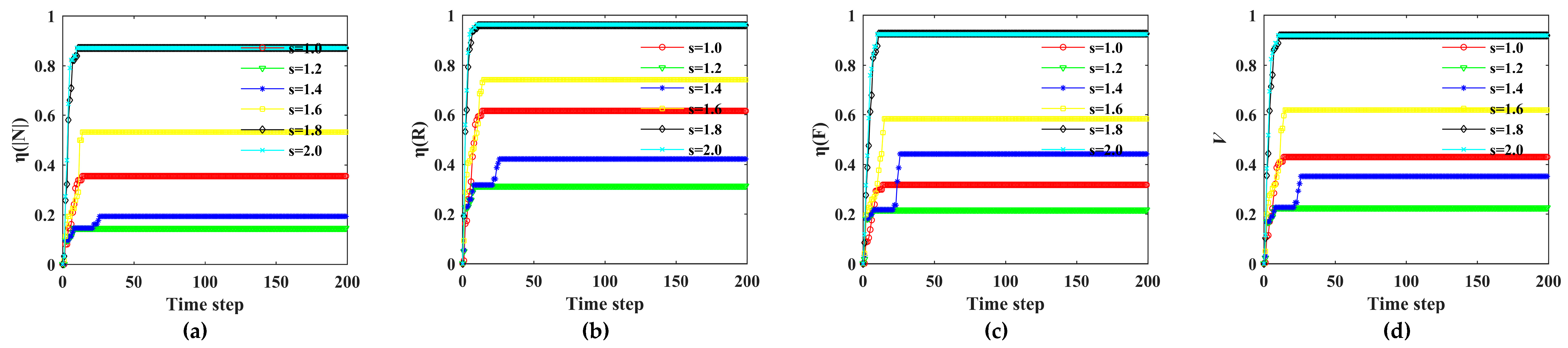
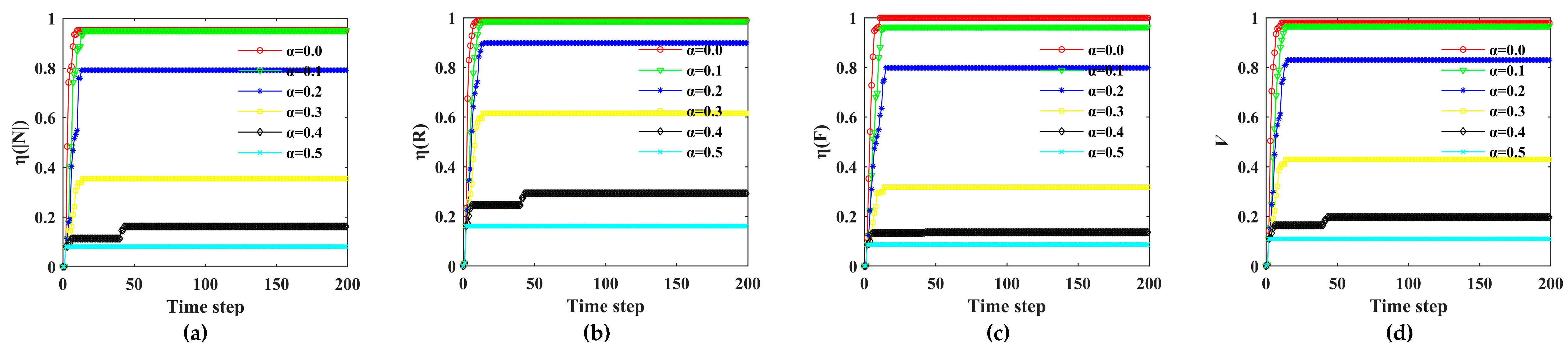
4.3. Vulnerability Analysis of Bus–Metro CBN under Rainstorm Conditions
5. Conclusions and Recommendations
Author Contributions
Funding
Acknowledgments
Conflicts of Interest
References
- Theofilatos, A.; Yannis, G. A review of the effect of traffic and weather characteristics on road safety. Accid. Anal. Prev. 2014, 72, 244–256. [Google Scholar] [CrossRef] [PubMed]
- Levy, J.I.; Buonocore, J.J.; Stackelberg, K.V. Evaluation of the public health impacts of traffic congestion: A health risk assessment. Environ. Health-Glob. 2010, 9, 65–65. [Google Scholar] [CrossRef] [PubMed]
- Margie, P.; Adnan, H. Road traffic injuries are a global public health problem. BMJ-Br. Med. J. 2002, 324, 1153–1153. [Google Scholar]
- Rampurkar, V.; Pentayya, P.; Mangalvedekar, H.A.; Kazi, F. Cascading failure analysis for Indian Power Grid. IEEE Trans. Smart Grid 2016, 7, 1951–1960. [Google Scholar] [CrossRef]
- Babaei, M.; Ghassemieh, H.; Jalili, M. Cascading failure tolerance of modular small-world networks. IEEE Trans. Circuits-II 2011, 58, 527–531. [Google Scholar] [CrossRef]
- Zhang, X.; Zhan, C.J.; Tse, C.K. Modeling the Dynamics of Cascading Failures in Power Systems. IEEE J. Emerg. Sel. Top. Circuits Syst. 2017, 7, 1–13. [Google Scholar] [CrossRef]
- Zheng, C.D.; Yan, J.F.; Meng, T. Cascading failures of interdependent networks with different k-core structures. Mod. Phys. Lett. B 2017, 31, 1750112. [Google Scholar] [CrossRef]
- Mirzasoleiman, B.; Babaei, M.; Jalili, M.; Safari, M. Cascaded failures in weighted networks. Phys. Rev. E Stat. Nonlinear Soft Matter Phys. 2011, 84, 046114. [Google Scholar] [CrossRef]
- Kornbluth, Y.; Lowinger, S.; Cwilich, G.; Buldyrev, S.V. Cascading failures in networks with proximate dependent nodes. Phys. Rev. E Stat. Nonlinear Soft Matter Phys. 2014, 89, 032808. [Google Scholar] [CrossRef]
- Song, M.L.; Weng, X.X.; Yao, S.S.; Chen, J. Research on the importance of the nodes of the cascading failure public transportation network based on complex network theory. J. Comput. Theor. Nanos 2016, 13, 5294–5304. [Google Scholar]
- He, T.; Zhu, N.; Hou, Z.; Xiong, G.X. A novel cascading failure model on city transit network. ICBEB 2016. [Google Scholar] [CrossRef]
- Jenelius, E.; Mattsson, L.G. Road network vulnerability analysis: Conceptualization, implementation and application. Comput. Environ. Urban 2015, 49, 136–147. [Google Scholar] [CrossRef]
- Husdal, J. Reliability and vulnerability versus costs and benefits. In Proceedings of the 2nd International Symposium Transportation Network Reliability (INSTR), Christchurch, New Zealand, 8–10 October 2004. [Google Scholar]
- Balijepalli, C.; Oppong, O. Measuring vulnerability of road network considering the extent of serviceability of critical road links in urban areas. J. Transp. Geogr. 2014, 39, 145–155. [Google Scholar] [CrossRef]
- Bell, M.G.H.; Kurauchi, F.; Perera, S.; Wong, W. Investigating transport network vulnerability by capacity weighted spectral analysis. Transp. Res. B-Math. 2017, 99, 251–266. [Google Scholar] [CrossRef]
- Alam, M.J.; Habib, M.A.; Quigley, K. Vulnerability in transport network during critical infrastructure renewal: Lessons learned from a dynamic traffic microsimulation model. Procedia Comput. Sci. 2017, 109, 616–623. [Google Scholar] [CrossRef]
- Ma, Y.H.; Zhang, Q.; Li, X.; Chen, S. Vulnerability analysis of bus transport network in Western China Cities. In Proceedings of the 2nd International Conference on Computer Science and Technology, Rome, Italy, 22–23 July 2019; pp. 455–459. [Google Scholar]
- Luskova, M.; Leitner, B.; Titko, M. Indicators of societal vulnerability related to impacts of extreme weather events on land transport infrastructure. In Proceedings of the 20th International Scientific Conference on Transport Means, Juodkrante, Lithuania, 5–7 October 2016; pp. 94–97. [Google Scholar]
- Tong, S.; Mather, P.; Fitzgerald, G.; McRae, D.; Verrall, K.; Walker, D. Assessing the vulnerability of eco-environmental health to climate change. Int. J. Environ. Res. Public Health 2010, 7, 546–564. [Google Scholar] [CrossRef] [PubMed]
- Brown, H.; Spickett, J.; Katscherian, D. A health impact assessment framework for assessing vulnerability and adaptation planning for climate change. Int. J. Environ. Res. Public Health 2014, 11, 12896. [Google Scholar] [CrossRef] [PubMed]
- Jenelius, E.; Mattsson, L.G. Developing a methodology for road network vulnerability analysis. Nectar Clust. 2006, 1, 1–9. [Google Scholar]
- Bernstein, A.; Bienstock, D.; Hay, D.; Uzunoglu, M.; Zussman, G. Power grid vulnerability to geographically correlated failures—Analysis and control implications. In Proceedings of the INFOCOM, Toronto, ON, Canada, 27 April–2 May 2014; pp. 2634–2642. [Google Scholar]
- Xia, Y.; Fan, J.; Hill, D. Cascading failure in Watts–Strogatz small-world networks. Phys. A 2012, 389, 1281–1285. [Google Scholar] [CrossRef]
- Berman, K.A. Vulnerability of scheduled networks and a generalization of Menger’s Theorem. Networks 2015, 28, 125–134. [Google Scholar] [CrossRef]
- Wang, J.W.; Rong, L.L. Edge-based-attack induced cascading failures on scale-free networks. Phys. A 2012, 388, 1731–1737. [Google Scholar] [CrossRef]
- Kermanshah, A.; Derrible, S. A geographical and multi-criteria vulnerability assessment of transportation networks against extreme earthquakes. Reliabil. Eng. Syst. Saf. 2016, 153, 39–49. [Google Scholar] [CrossRef]
- Mishra, B.K.; Singh, A.K. Two Quarantine Models on the Attack of Malicious Objects in Computer Network. Math. Probl. Eng. 2011, 2012, 1–14. [Google Scholar] [CrossRef]
- Pu, C.L.; Cui, W. Vulnerability of complex networks under path-based attacks. Phys. A 2015, 419, 622–629. [Google Scholar] [CrossRef]
- Newman, M.E.; Forrest, S.; Balthrop, J. Email networks and the spread of computer viruses. Phys. Rev. E Stat. Nonlinear Soft Matter Phys. 2002, 66, 035101. [Google Scholar] [CrossRef] [PubMed]
- Hua, M.G.; Cheng, P.; Fei, J.T.; Chen, J.F. Network-Based Robust H∞ Filtering for the Uncertain Systems with Sensor Failures and Noise Disturbance. Math. Probl. Eng. 2012. [Google Scholar] [CrossRef]
- Li, M.; Zhao, W. Industrial Noise. Math. Probl. Eng. 2012, 2012, 939–955. [Google Scholar]
- Wilkinson, S.M.; Dunn, S.; Ma, S. The vulnerability of the European air traffic network to spatial hazards. Nat. Hazards 2012, 60, 1027–1036. [Google Scholar] [CrossRef]
- Hines, P.; Cotilla-Sanchez, E.; Blumsack, S. Do topological models provide good information about electricity infrastructure vulnerability? Chaos 2010, 20, 033122. [Google Scholar] [CrossRef]
- Ouyang, M. Comparisons of purely topological model, betweenness based model and direct current power flow model to analyze power grid vulnerability. Chaos 2013, 23, 293–296. [Google Scholar] [CrossRef]
- Ferber, C.V.; Holovatch, T.; Holovatch, Y. Attack vulnerability of public transport networks. Traffic Granular Flow 2007, 2009, 721–731. [Google Scholar]
- Berche, B.; Ferber, C.V.; Holovatch, T.; Holovatch, Y. Resilience of public transport networks against attacks. Eur. Phys. J. B 2009, 71, 125–137. [Google Scholar] [CrossRef]
- Yin, H.Y.; Xu, L.Q. Measuring the structural vulnerability of road Network: A network efficiency perspective. J. Shanghai Jiaotong Univ. 2010, 15, 736–742. [Google Scholar] [CrossRef]
- Adachi, T.; Ellingwood, B.R. Serviceability of earthquake-damaged water systems: Effects of electrical power availability and power backup systems on system vulnerability. Reliabil. Eng. Syst. Saf. 2008, 93, 78–88. [Google Scholar] [CrossRef]
- Johansson, J.; Hassel, H. An approach for modelling interdependent infrastructures in the context of vulnerability analysis. Reliabil. Eng. Syst. Saf. 2010, 95, 1335–1344. [Google Scholar] [CrossRef]
- Ouyang, M.; Hong, L.; Mao, Z.J.; Yu, M.H.; Qi, F. A methodological approach to analyze vulnerability of interdependent infrastructures. Simul. Model. Pract. Theory 2009, 17, 817–828. [Google Scholar] [CrossRef]
- Leonardo, D.O.; Craig, J.I.; Goodno, B.J. Seismic response of critical interdependent networks. Earthq. Eng. Struct. D 2010, 36, 285–306. [Google Scholar]
- Soh, H.; Lim, S.; Zhang, T.; Fu, X.; Lee, G.K.; Hung, T.G.; Di, P.; Prakasam, S.; Wong, L. Weighted complex network analysis of travel routes on the Singapore public transportation system. Phys. A 2010, 389, 5852–5863. [Google Scholar] [CrossRef]
- Huang, A.L.; Guan, W.; Mao, B.H.; Zang, G.Z. Statistical analysis of weighted complex network in Beijing public transit routes system based on passenger flow. J. Transp. Syst. Eng. Inf. Technol. 2013, 13, 198–204. [Google Scholar]
- El-Rashidy, R.A.; Grant-Muller, S.M. An assessment method for highway network vulnerability. J. Transp. Geogr. 2014, 34, 34–43. [Google Scholar] [CrossRef]
- Xing, R.R.; Yang, Q.F.; Zheng, L.L. Research on Cascading Failure Model of Urban Regional Traffic Network under Random Attacks. Discrete Dyn. Nat. Soc. 2018, 2018, 1915695. [Google Scholar] [CrossRef]
- Wu, J.J.; Sun, H.J.; Gao, Z.Y. Cascading failures on weighted urban traffic equilibrium networks. Phys. A 2007, 386, 407–413. [Google Scholar] [CrossRef]
- Zheng, J.F.; Gao, Z.Y.; Zhao, X.M. Modeling cascading failures in congested complex networks. Phys. A 2007, 385, 700–706. [Google Scholar] [CrossRef]
- Zhang, L.; Fu, B.B.; Li, Y.X. Cascading failure of urban weighted public transit network under single station happening emergency. Procedia Eng. 2016, 137, 259–266. [Google Scholar] [CrossRef]
- Zhang, L.; Fu, B.B.; Li, S.B. Cascading failures coupled model of interdependent double layered public transit network. Int. J. Mod. Phys. C 2016, 27. [Google Scholar] [CrossRef]
- Yang, Y.; Huang, A.; Guan, W. Statistic properties and cascading failures in a coupled transit network consisting of bus and subway systems. Int. J. Mod. Phys. B 2014, 28. [Google Scholar] [CrossRef]
- Buldyrev, S.V.; Parshani, R.; Paul, G.; Stanley, H.E.; Havlin, S. Catastrophic cascade of failures in interdependent networks. Nature 2010, 464, 1025–1028. [Google Scholar] [CrossRef]
- Trenberth, K.E. Atmosphere moisture residence times and cycling: Implications for rainfall rates with climate change. Clim. Chang. 1998, 39, 667–694. [Google Scholar] [CrossRef]
- Frich, P.; Alexander, L.V.; Della-Marta, P.M.; Gleason, B.; Haylock, M.; Tank, A.K.; Peterson, T. Observed coherent changes in climatic extremes during the second half of the twentieth century. Clim. Res. 2002, 19, 193–212. [Google Scholar] [CrossRef]
- Klein Tank A, M.G.; Konnen, G.P. Trends in indices of daily temperature and precipitation extremes in Europe, 1946–1999. J. Clim. 2003, 16, 3665–3680. [Google Scholar] [CrossRef]
- Groisman, P.Y.; Knight, R.W.; Karl, T.R.; Easterling, D.R.; Sun, B.; Lawrimore, J.H. Contemporary Changes of the Hydrological Cycle over the Contiguous United States: Trends Derived from In Situ Observations. J. Hydrometeorol. 2004, 5, 64–85. [Google Scholar] [CrossRef]
- Brunetti, M. Changes in daily precipitation frequency and distribution in Italy over the last 120 years. J. Geophys. Res. 2004, 109, D05102. [Google Scholar] [CrossRef]
- Papadakis, M. Consequences of Extreme Weather. EGU General Assembly 2012, 14, 11936. [Google Scholar]
- Goel, G.; Sachdeva, S.N. Impact of rainwater on bituminous road surfacing. In Development of Water Resources in India; Springer: Cham, Switzerland, 2017. [Google Scholar]
- Lyu, H.M.; Sun, W.J.; Shen, S.L.; Arulrajah, A. Flood risk assessment in metro systems of mega-cities using a GIS-based modeling approach. Sci. Total Environ. 2018, 626, 1012. [Google Scholar] [CrossRef] [PubMed]
- Xu, F.; He, Z.; Sha, Z.; Zhuang, L.; Sun, W. Survey the impact of different rainfall intensities on urban road traffic operations using Macroscopic Fundamental Diagram. In Proceedings of the International IEEE Conference on Intelligent Transportation Systems, Rio de Janeiro, Brazil, 1–4 November 2014. [Google Scholar]
- Bi, S.; Zhao, Z.; Wang, G.; Kong, L.; Diao, Q.; Han, C.; Sun, D. Research on travel time prediction under the condition of urban extreme weather in overpass area. Adv. Mater. Res. 2014, 989–994, 5565–5570. [Google Scholar] [CrossRef]
- Dong, J.S.; Wu, Y.W.; Lu, Q.C. Road Network Topology Vulnerability Indentification Considering the Intensity of Rainfall in Urban Areas. J. Transp. Syst. Eng. Inf. Technol. 2015, 15, 109–122. [Google Scholar]
- Yang, P.G.; Jin, J.; Zhao, D.S. An Urban Vulnerability Study Based on Historical Flood Data: A Case Study of Beijing. Scientia Geographica Sinica 2016, 36, 733–741. [Google Scholar]
- Huang, A.; Zhang, H.M.; Guan, W.; Yang, Y.; Zong, G. Cascading failures in weighted complex networks of transit systems based on coupled map lattices. Math. Probl. Eng. 2015, 2015, 1–16. [Google Scholar] [CrossRef]
- Peng, X.Z.; Li, B.Y.; Yao, H. A cascading invulnerability analysis for multi-layered networks. Adv. Mater. 2013, 846–847, 853–857. [Google Scholar] [CrossRef]
- Ren, F.; Zhao, T.; Wang, H. Risk and resilience analysis of complex network systems considering cascading failure and recovery strategy based on coupled map lattices. Math. Probl. Eng. 2015, 2015, 761818. [Google Scholar] [CrossRef]
- Motter, A.E.; Lai, Y.C. Cascade-based attacks on complex networks. Phys. Rev. E 2002, 66, 065102. [Google Scholar] [CrossRef] [PubMed]
- Nagatani, T. Self-organized criticality in 1D traffic flow model with inflow or outflow. J Phys. A 1995, 28, L119. [Google Scholar] [CrossRef]
- Pesheva, N.; Brankov, J.; Valkov, N. Self-organized criticality in $1rm D$ stochastic traffic flow model with a speed limit. Rep. Math. Phys. 1997, 40, 509–520. [Google Scholar] [CrossRef]
- Bak, P.; Tang, C.; Wiesenefld, K. Self-organized criticality: An explanation of l/f noise. Phys. Rev. Lett. 1987, 59, 3810–384. [Google Scholar] [CrossRef] [PubMed]
- Wu, J.; Gao, Z.; Sun, H.; Huang, H. Urban transit system as a scale-free network. Mod. Phys. Lett. B 2008, 18, 1043–1049. [Google Scholar] [CrossRef]
- Sienkiewicz, J.; Holyst, J.A. Statistical analysis of 22 public transport networks in Poland. Phys. Rev. E Stat. Nonlinear Soft Matter Phys. 2005, 72, 046127. [Google Scholar] [CrossRef] [PubMed]
- Derrible, S.; Kennedy, C. The complexity and robustness of metro networks. Phys. A 2010, 389, 3678–3691. [Google Scholar] [CrossRef]
- Huang, A. Study on Structure and Dynamic Behaviour in Weighted Complex Public Transit Network Based on Passenger Flow; Beijing Jiaotong University: Beijing, China, 2014. [Google Scholar]
- Moreno, Y.; Gmez, J.B.; Pacheco, A.E. Instability of scale-free networks under node-breaking avalanches. Europhys. Lett. 2002, 58, 630–636. [Google Scholar] [CrossRef]
- Watts, D.J. A simple model of global cascades on random networks. Pnas 2002, 99, 5766–5771. [Google Scholar] [CrossRef]
- Bonabeau, E. Sandpile dynamics on random graphs. J. Phys. Soc. Jpn. 1995, 64, 327–328. [Google Scholar] [CrossRef]
- Kaneko, K. Coupled Map Lattices; World Scientific: Singapore, 1992. [Google Scholar]
- Shao, J.; Buldyrev, S.V.; Havlin, S.; Stanley, H.E. Cascade of failures in coupled network systems with multiple support-dependence relations. Phys. Rev. E 2011, 83, 036116. [Google Scholar] [CrossRef] [PubMed]
- Bevers, M.; Flather, C.H. Numerically exploring habitat fragmentation effects on populations using cell-based coupled map lattices. Theory Popul. Biol. 1999, 55, 61. [Google Scholar] [CrossRef] [PubMed]
- Willeboordse, F.H.; Kaneko, K. Pattern dynamics of a coupled map lattice for open flow. Phys. D 1994, 86, 428–455. [Google Scholar] [CrossRef]
- Chen, H.; Zheng, Z.; Chen, Z.; Bi, X. A lattice gas automata model for the coupled heat transfer and chemical reaction of gas flow around and through a porous circular cylinder. Entropy 2015, 18, 2. [Google Scholar] [CrossRef]
- Ahmed, E.; Abdusalam, H.A.; Fahmy, E.S. On telegraph reaction diffusion and coupled map latice in some biological systems. Int. J. Mod. Phys. C 2001, 12, 717–726. [Google Scholar] [CrossRef]
- Qian, Y.; Wang, B.; Xue, Y.; Zeng, J.; Wang, N. A simulation of the cascading failure of a complex network model by considering the characteristics of road traffic conditions. Nonlinear Dyn. 2015, 80, 413–420. [Google Scholar] [CrossRef]
- Lhaksmana, K.M.; Murakami, Y.; Ishida, T. Analysis of large-scale service network tolerance to cascading failure. IEEE Int. Things 2017, 3, 1159–1170. [Google Scholar] [CrossRef]
- Disbro, J.E.; Frame, M. Traffic flow theory and chaotic behaviour. Transp. Res. Rec. 1989, 1225, 109–115. [Google Scholar]
- Johanns, R.D.; Roozemond, D.A. An Object Based Traffic Control Strategy: A Chaos Theory Approach with an Object-Oriented Implementation; Elsevier Science Ltd.: Amsterdam, The Netherlands, 1993. [Google Scholar]
- Du, Z.; Wang, R.; Ji, C. Study of chaos’ state of traffic flow in logistic mapping. TST 2005, 209, 78–80. [Google Scholar]
- Cats, O.; Jenelius, E. Beyond a complete failure: The impact of partial capacity degradation on public transport network vulnerability. In Proceedings of the 6th INSTR, Nara, Japan, 2–3 August 2015. [Google Scholar]
- Feng, H.F.; Cai-Hong, L.I.; Wang, R. Vulnerability study for public transport network of valley city: Case of Lanzhou. J. Transp. Syst. Eng. Inf. Technol. 2016, 16, 217–222. [Google Scholar]
- Kaneko, K. Overview of coupled map lattices. Chaos Interdiscip. J. Nonlinear Sci. 1992, 2, 279. [Google Scholar] [CrossRef] [PubMed]
- Dey, P.; Mehra, R.; Kazi, F.; Wagh, S.; Singh, N.M. Impact of Topology on the Propagation of Cascading Failure in Power Grid. IEEE T SMART GRID 2017, 7, 1970–1978. [Google Scholar]
- Xiao, L.; Wang, H.L. Urban public transport network study of cascading failure. Mach. Electron. 2010, 17, 72–88. [Google Scholar]
- Cheng-Bing, L.I.; Wei, L.; Gao, W. Invulnerability of urban agglomeration compound traffic network against cascading failure. J. Highw. Transp. Res. Dev. 2018, 94, 77–87. [Google Scholar]
- Bompard, E.; Estebsari, A.; Huang, T.; Fulli, G. A framework for analyzing cascading failure in large interconnected power systems: A post-contingency evolution simulator. Int. J. Electr. Power 2016, 81, 12–21. [Google Scholar] [CrossRef]
- Malik, S.U.; Srinivasan, S.K.; Khan, S.U. Convergence time analysis of open shortest path first routing protocol in internet scale networks. Electron. Lett. 2012, 48, 1188–1190. [Google Scholar] [CrossRef]
- Strogatz, S.H. Network Robustness and Fragility: Percolation on Random Graphs. Phys. Rev. Lett. 2000, 85, 5468. [Google Scholar]
- Dobson, I.; Carreras, B.A.; Lynch, V.E.; Newman, D.E. Complex systems analysis of series of blackouts: Cascading failure, critical points, and self-organization. Chaos 2007, 17, 967–979. [Google Scholar] [CrossRef]
- Dueñas-Osorio, L.; Vemuru, S.M. Cascading failures in complex infrastructure systems. Struct. Saf. 2009, 31, 157–167. [Google Scholar] [CrossRef]


| Intensities of Rainfall | Influence on Bus–Metro CBN Operation |
|---|---|
| ≥50 mm/24 h | Reduces the friction coefficient of road surfaces and increases the incidence of bus accidents. |
| ≥100 mm/24 h | Reduces the friction coefficient of road surfaces and increases the incidence of bus accidents; partial rail transit interruptions and delay. |
| ≥150 mm/24 h | Bus outage, delays, bus lines shrinkage; partial rail transit interruptions and delay, with orbiting system destroyed. |
| Bus Stop | Bus Lines Operating at the Stop | Whether is a Transfer Stop |
|---|---|---|
| BAISHULIN | 258, 309, 706, 707 | No |
| HONGHUJIE | 102, 103, 10, 12, 235, 28, 301, 506, 606, 702 | Yes |
| … | … | … |
| LUOMASHI | 706, 707 | No |
| XIWUYUAN | 107, 703, 702 | No |
| Bus line | No. of bus stops on the line | No. of transfer stops on the line |
| 4 | 8 | 3 |
| 20 | 4 | 1 |
| … | … | … |
| 182 | 8 | 1 |
| 606 | 8 | 5 |
| Metro station | Metro lines running through station | Whether is a transfer station |
| ANYUANMEN | 2 | No |
| BEIDAJIE | 1, 2 | Yes |
| … | … | … |
| ZHONGLOU | 2 | No |
| WULUKOU | 1 | No |
| Metro line | No. of metro stations on the line | No. of transfer stations on the line |
| 1 | 5 | 1 |
| 2 | 4 | 1 |
| Network | Nodes | Edges | Average Degree | Average Path Length | Clustering Coefficient |
|---|---|---|---|---|---|
| Bus | 54 | 85 | 3.148 | 4.593 | 0.201 |
| Metro | 8 | 7 | 1.750 | 2.286 | 0.000 |
| Bus–Metro | 62 | 99 | 3.194 | 4.480 | 0.174 |
| Scenario | s | α | ε1 | ε2 | Object of Research |
|---|---|---|---|---|---|
| 1 | 1.00 | 0.3 | 0.2 | 0.2 | Impact of rainstorm on Bus–Metro CBN |
| 2 | 1.20 | 0.3 | 0.2 | 0.2 | |
| 3 | 1.40 | 0.3 | 0.2 | 0.2 | |
| 4 | 1.60 | 0.3 | 0.2 | 0.2 | |
| 5 | 1.80 | 0.3 | 0.2 | 0.2 | |
| 6 | 2.00 | 0.3 | 0.2 | 0.2 | |
| 7 | 1.00 | 0.0 | 0.2 | 0.2 | Impact of capacity tolerance on Bus–Metro CBN |
| 8 | 1.00 | 0.1 | 0.2 | 0.2 | |
| 9 | 1.00 | 0.2 | 0.2 | 0.2 | |
| 10 | 1.00 | 0.3 | 0.2 | 0.2 | |
| 11 | 1.00 | 0.4 | 0.2 | 0.2 | |
| 12 | 1.00 | 0.5 | 0.2 | 0.2 | |
| 13 | 1.00 | 0.3 | 0.2 | 0.2 | Influence of node coupling strength on Bus–Metro CBN |
| 14 | 1.00 | 0.3 | 0.4 | 0.2 | |
| 15 | 1.00 | 0.3 | 0.6 | 0.2 | |
| 16 | 1.00 | 0.3 | 0.8 | 0.2 | |
| 17 | 1.00 | 0.3 | 0.2 | 0.2 | Influence of edge coupling strength on Bus–Metro CBN |
| 18 | 1.00 | 0.3 | 0.2 | 0.4 | |
| 19 | 1.00 | 0.3 | 0.2 | 0.6 | |
| 20 | 1.00 | 0.3 | 0.2 | 0.8 |
| Scenario | Variable | Value of Variable | Convergence Time (Step) | η(|N|) | η(R) | η(F) | V |
|---|---|---|---|---|---|---|---|
| 1 | s | 1.00 | 14 | 0.355 | 0.615 | 0.318 | 0.429 |
| 2 | 1.20 | 8 | 0.145 | 0.314 | 0.217 | 0.227 | |
| 3 | 1.40 | 26 | 0.194 | 0.421 | 0.441 | 0.352 | |
| 4 | 1.60 | 15 | 0.532 | 0.740 | 0.583 | 0.618 | |
| 5 | 1.80 | 11 | 0.871 | 0.959 | 0.926 | 0.919 | |
| 6 | 2.00 | 10 | 0.871 | 0.962 | 0.923 | 0.919 | |
| 7 | α | 0.0 | 11 | 0.952 | 0.989 | 1.000 | 0.980 |
| 8 | 0.1 | 15 | 0.952 | 0.988 | 0.964 | 0.968 | |
| 9 | 0.2 | 15 | 0.790 | 0.898 | 0.799 | 0.829 | |
| 10 | 0.3 | 14 | 0.355 | 0.615 | 0.318 | 0.429 | |
| 11 | 0.4 | 43 | 0.161 | 0.293 | 0.136 | 0.197 | |
| 12 | 0.5 | 2 | 0.081 | 0.161 | 0.086 | 0.109 | |
| 7 | ε1 | 0.2 | 14 | 0.355 | 0.615 | 0.318 | 0.429 |
| 8 | 0.4 | 14 | 0.565 | 0.755 | 0.503 | 0.608 | |
| 9 | 0.6 | 14 | 0.565 | 0.766 | 0.542 | 0.624 | |
| 10 | 0.8 | 14 | 0.565 | 0.766 | 0.542 | 0.624 | |
| 11 | ε2 | 0.2 | 14 | 0.355 | 0.615 | 0.318 | 0.429 |
| 12 | 0.4 | 14 | 0.339 | 0.605 | 0.316 | 0.420 | |
| 13 | 0.6 | 14 | 0.403 | 0.656 | 0.327 | 0.462 | |
| 14 | 0.8 | 19 | 0.661 | 0.847 | 0.589 | 0.699 |
© 2019 by the authors. Licensee MDPI, Basel, Switzerland. This article is an open access article distributed under the terms and conditions of the Creative Commons Attribution (CC BY) license (http://creativecommons.org/licenses/by/4.0/).
Share and Cite
Ma, F.; Liu, F.; Yuen, K.F.; Lai, P.; Sun, Q.; Li, X. Cascading Failures and Vulnerability Evolution in Bus–Metro Complex Bilayer Networks under Rainstorm Weather Conditions. Int. J. Environ. Res. Public Health 2019, 16, 329. https://doi.org/10.3390/ijerph16030329
Ma F, Liu F, Yuen KF, Lai P, Sun Q, Li X. Cascading Failures and Vulnerability Evolution in Bus–Metro Complex Bilayer Networks under Rainstorm Weather Conditions. International Journal of Environmental Research and Public Health. 2019; 16(3):329. https://doi.org/10.3390/ijerph16030329
Chicago/Turabian StyleMa, Fei, Fei Liu, Kum Fai Yuen, Polin Lai, Qipeng Sun, and Xiaodan Li. 2019. "Cascading Failures and Vulnerability Evolution in Bus–Metro Complex Bilayer Networks under Rainstorm Weather Conditions" International Journal of Environmental Research and Public Health 16, no. 3: 329. https://doi.org/10.3390/ijerph16030329
APA StyleMa, F., Liu, F., Yuen, K. F., Lai, P., Sun, Q., & Li, X. (2019). Cascading Failures and Vulnerability Evolution in Bus–Metro Complex Bilayer Networks under Rainstorm Weather Conditions. International Journal of Environmental Research and Public Health, 16(3), 329. https://doi.org/10.3390/ijerph16030329