Traffic Simulation Analysis on Running Speed in a Connected Vehicles Environment


Abstract
1. Introduction
2. Model Development
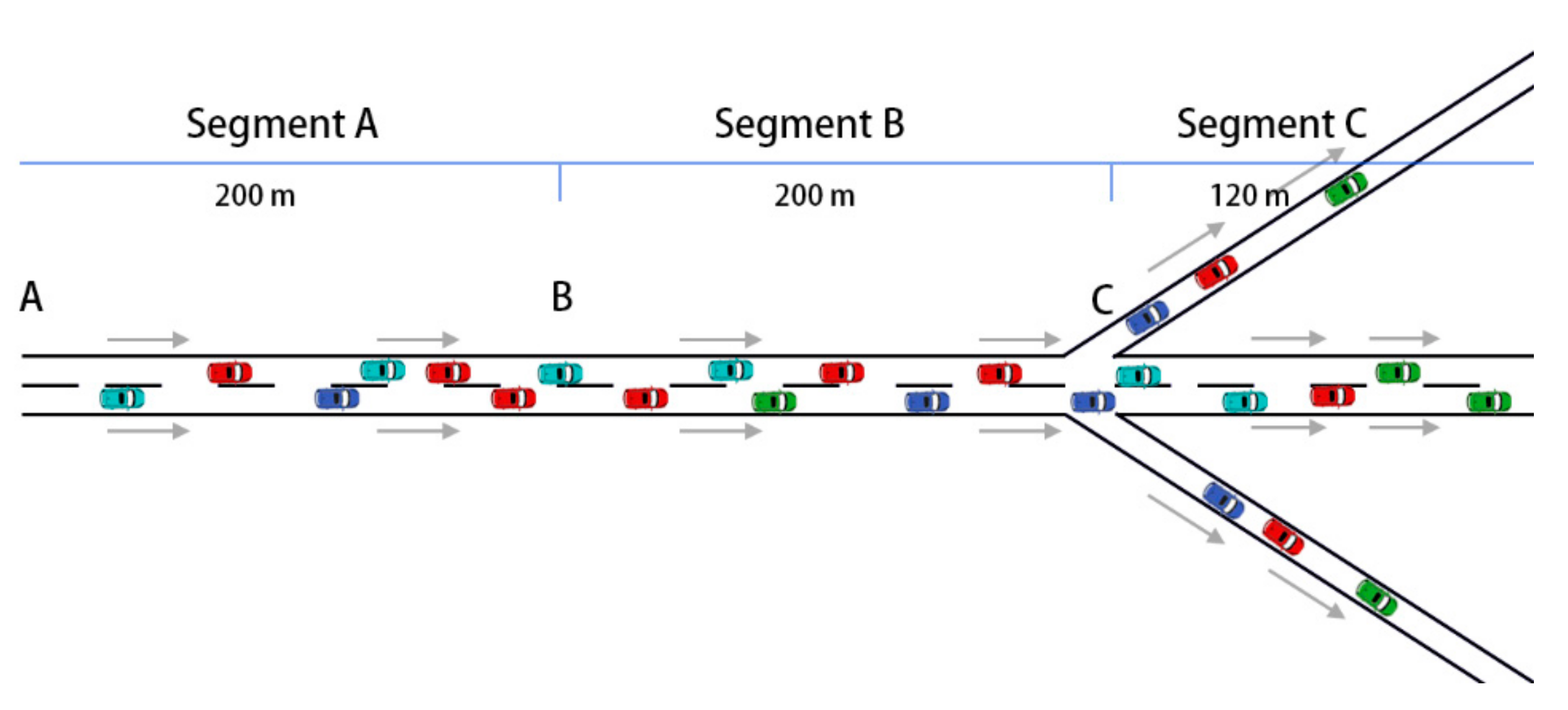
2.1. Road Model Based on VISSIM
2.2. Optimization Speed Model Based on MATLAB
2.2.1. Optimal Speed Control Strategy
- i = vehicle number (i = 1, 2, 3…)
- n = total number of vehicles in Segment B
- t = the tth time step
- ai,t = acceleration of vehicle i at time step t
- vi,t = velocity of vehicle i at time step t
- xi,t = distance of vehicle i at time step t to the merging point
- vmax = speed limit (here vmax = 20 m/s; the design speed is 50 km/h)
- Gmin = minimum distance gap (here Gmin = 10 m, considering driving safety)
- amin = minimum acceleration rate (here amin = −5 m/s2, estimated based on the measured data)
- amax = maximum acceleration rate (here amax = −5 m/s2, estimated based on the measured data)
- C = the average total acceleration of all the situations, which is calculated in advance
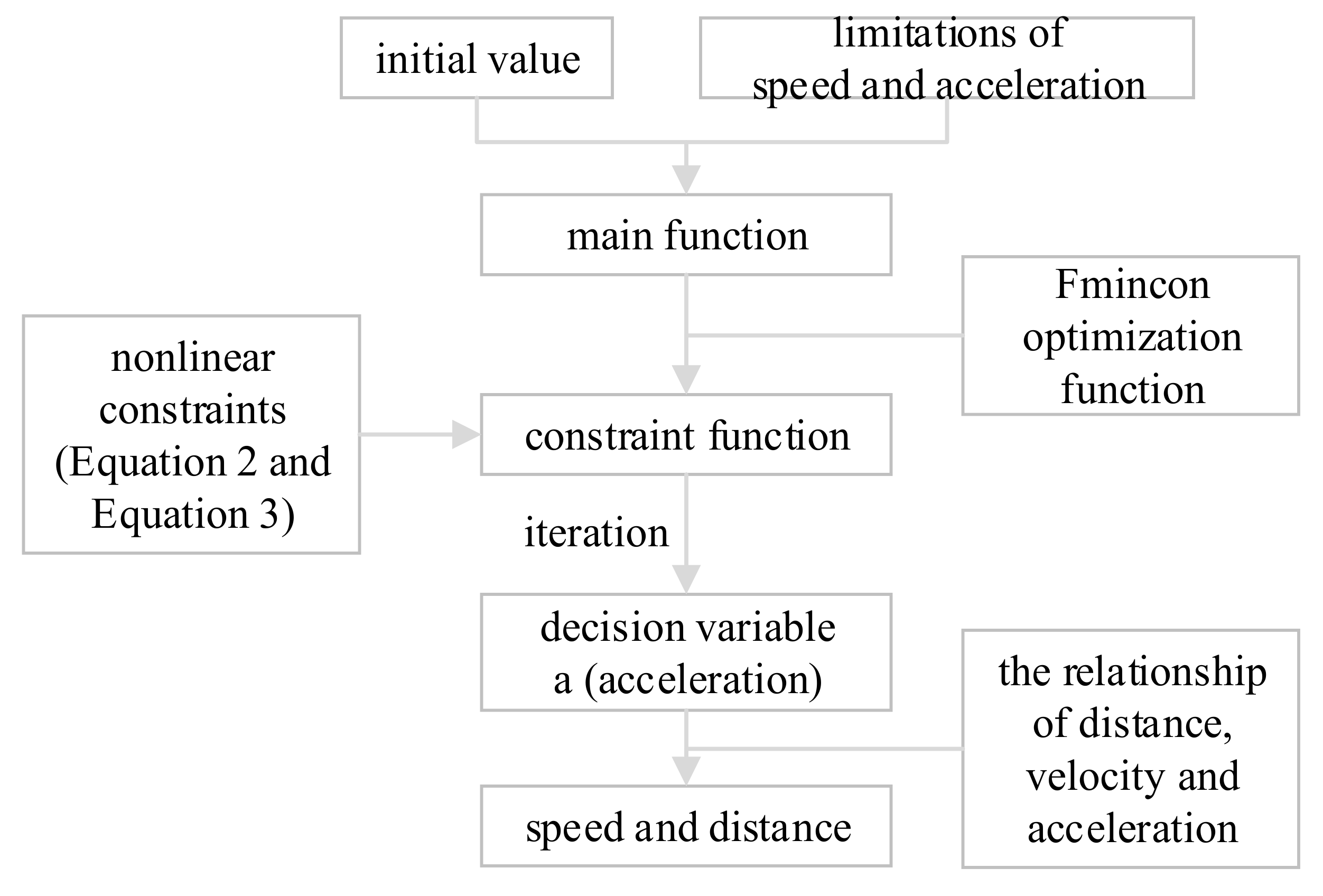
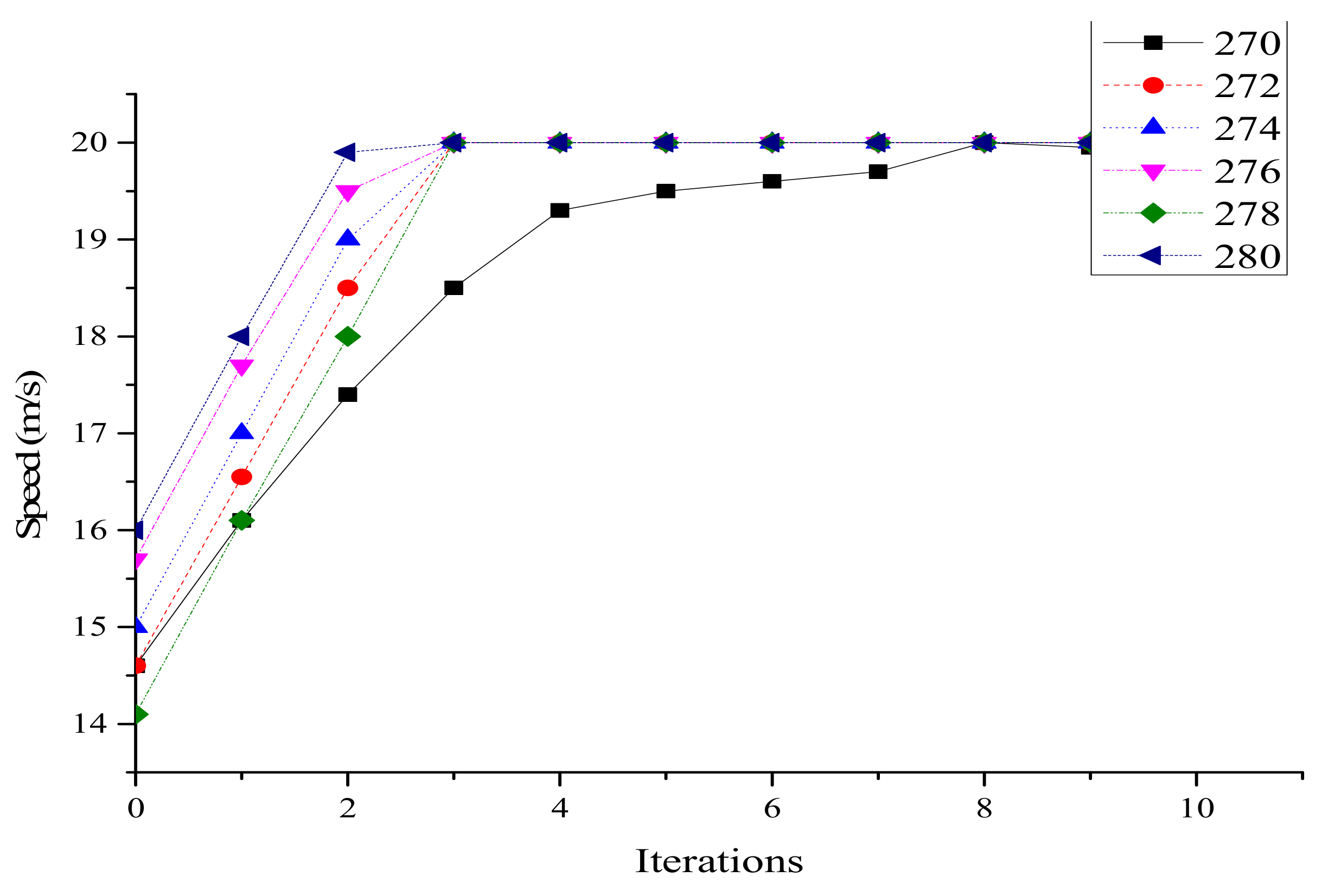
2.2.2. Using MATLAB to Implement Optimization Speed Model
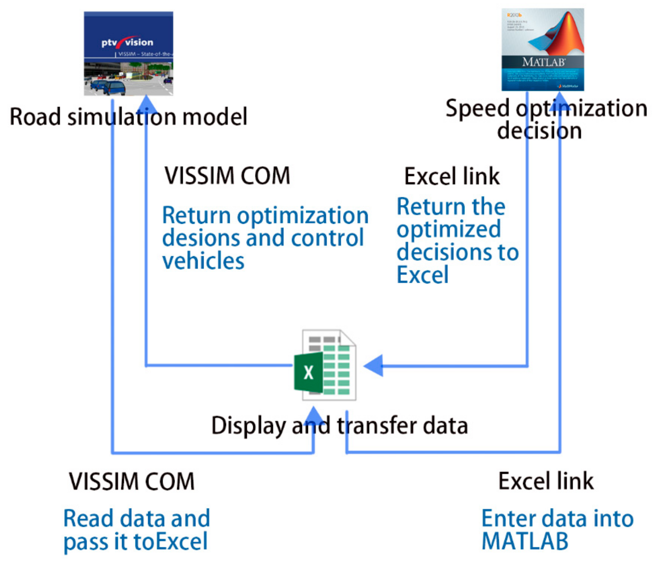
2.3. Simulation Framework
- 1
- The road model and the traffic environment were established in VISSIM for micro simulation.
- 2
- The experiment results were read in the VISSIM’s COM (Cluster Communication Port) interface. Specifically, the speed, acceleration, and position of the vehicles in Segment A were read per second. Such an advanced simulation was handled through the VISSIM–COM interface and implemented in MATLAB.
- 3
- Excel was adopted as the intermediate program to realize data transmission of VISSIM and MATLAB. MATLAB was called through the Excel link interface, and the simulation data was transferred between VISSIM and MATLAB.
- 4
- The MATLAB optimization speed model was adopted with the Fmincon algorithm to optimize the average running speed. Then MATLAB returned the output value per second (i.e., the acceleration), and stored it in Excel via Excel link [22].
- 5
- The optimization decision was read in Excel through the COM interface, and the COM interface was connected with Excel. A C++ program was written to control the vehicles as the kernel of the model [23].
- 6
- The instant simulation of VISSIM was based on the optimized decision, by which the vehicle exchanged information instantly under the connected state and determines its own speed and acceleration. Then VISSIM output the simulation evaluation data.
3. Results
3.1. Model Verification
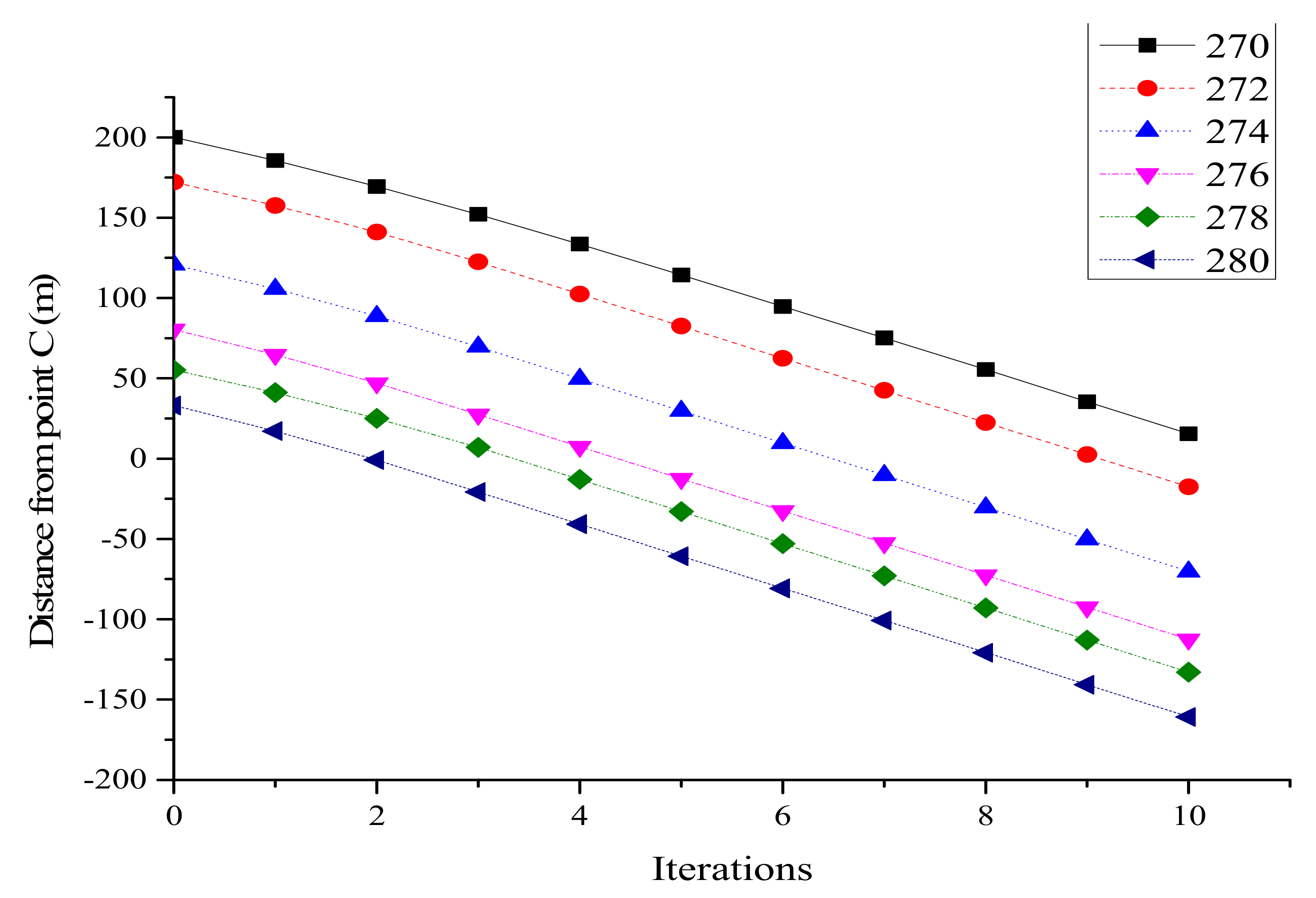
3.1.1. Case 1
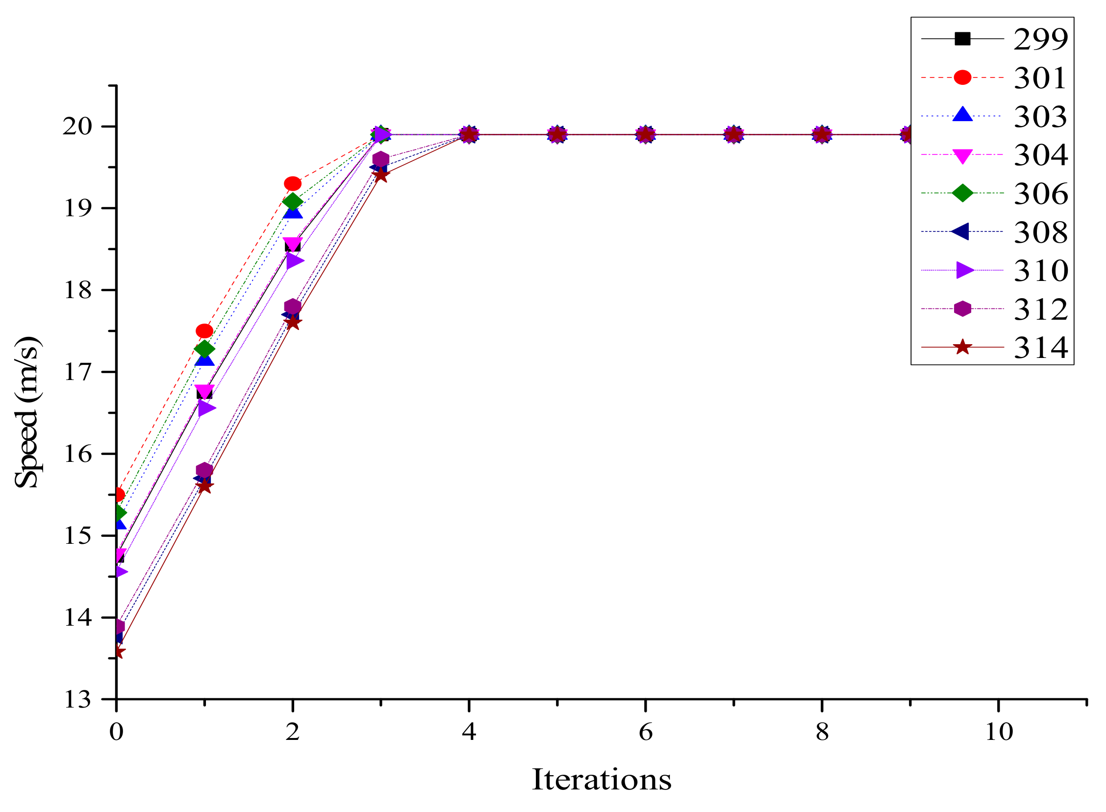
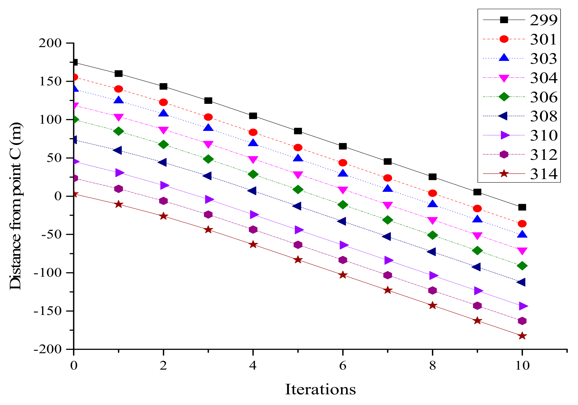
3.1.2. Case 2
3.2. Speed Optimization Results
3.2.1. Analysis on Data Collection Points
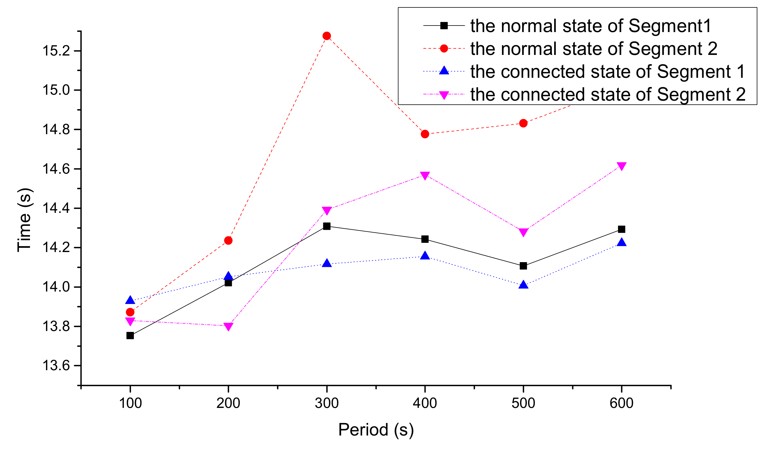
3.2.2. Analysis on Travel Time and Delay Time
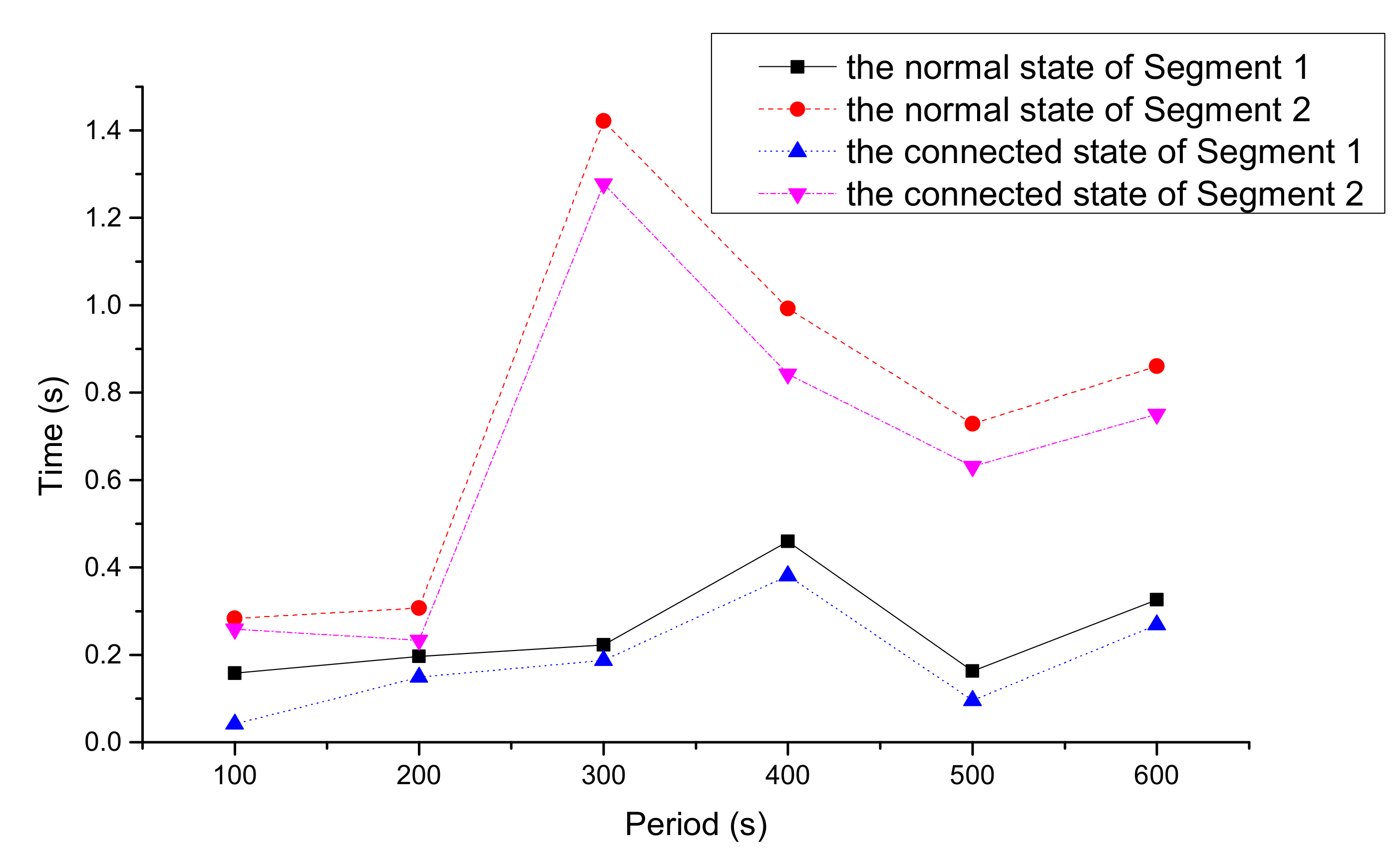
3.2.3. Analysis of the Mixed Traffic Flow in the Normal and the Connected States
4. Discussion
- 1.
- Most vehicles’ speed in the crowded traffic flow tended to be zero, which brought negative effects on the accuracy of speed analysis.
- 2.
- The vehicle distance was limited to 10 m in this model, but it was not true when the traffic was blocked. As a result, it is not conductive to analyzing queue length and vehicles’ passing time.
5. Conclusions
- (1)
- The running speed in the connected state is 4 km/h larger than that in the normal state. It proves that the fully-connected environment can improve running speed significantly.
- (2)
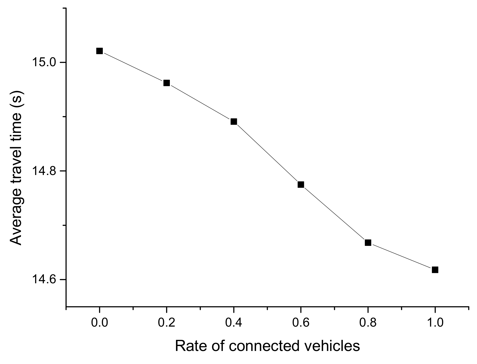
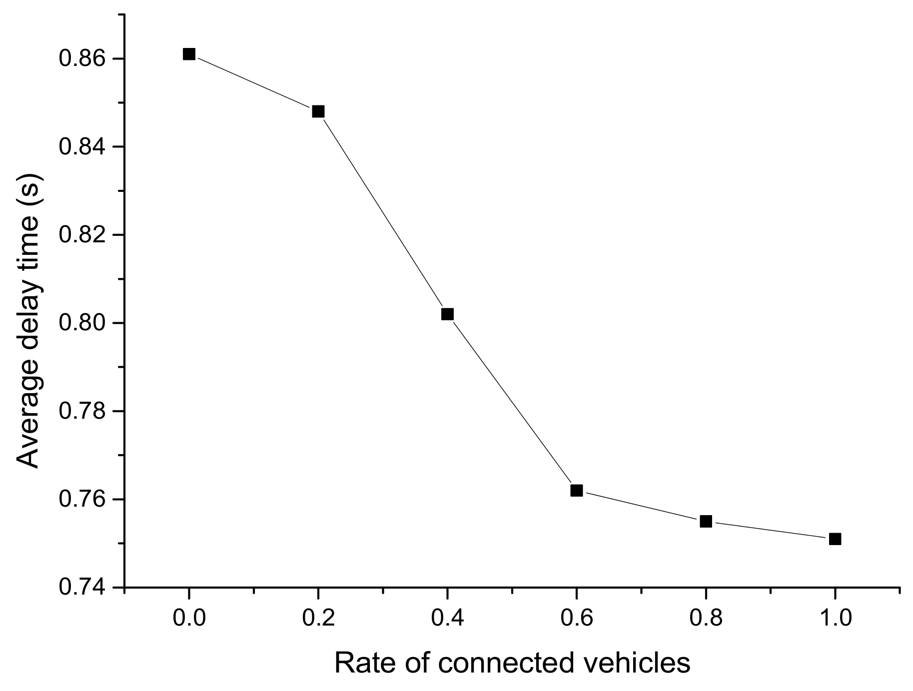
- The average total travel time and delay time of changing lanes or diverging decrease by 5.34% and 16.76% in the connected state, respectively. It shows that the fully-connected environment can make good use of the existing road infrastructure and improve traffic efficiency.
- (3)
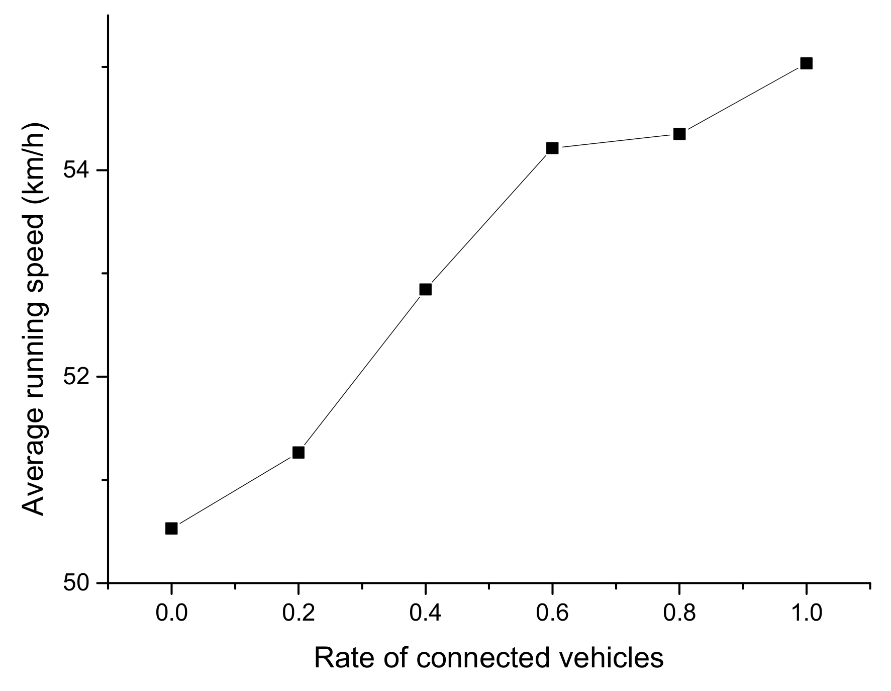
- The optimal CV market penetrating rate is 0.6. At such a rate, the running speed, travel time, and delay time is 56.21 km/h, 14.77 s, and 0.76 s, respectively.
Author Contributions
Funding
Conflicts of Interest
References
- Baber, J.; Kolodko, J.; Noel, T.; Parent, M.; Vlacic, L. Cooperative autonomous driving: Intelligent vehicles sharing city roads. IEEE Robot. Autom. Mag. 2005, 12, 44–49. [Google Scholar] [CrossRef]
- Kirkpatrick, K. The moral challenges of driverless cars. Commun. ACM 2015, 58, 19–20. [Google Scholar] [CrossRef]
- Duan, J.M.; Zheng, K.H.; Long-Jie, L.I.; Shi, L.X. Environmental perception of multi-layer laser radar in driverless car. J. Univ. Sci. Technol. B 2016, 40, 1891–1898. [Google Scholar]
- Oliveira, M.; Santos, V.; Sappa, A.D.; Dias, P.; Moreira, A.P. Incremental scenario representations for autonomous driving using geometric polygonal primitives. Robot. Auton. Syst. 2016, 83, 312–325. [Google Scholar] [CrossRef]
- Raimondi, F.M.; Melluso, M. Fuzzy adaptive EKF motion control for non-holonomic and underactuated cars with parametric and non-parametric uncertainties. IEZT Control Theory Appl. 2007, 1, 1311–1321. [Google Scholar] [CrossRef]
- Kang, M.W.; Wang, S.; Jha, M.K.; Chen, C.C.; Schonfeld, P. A Simulation Framework for the Path Planning of Driverless Autonomous Systems. In Proceedings of the First International Symposium on Uncertainty Modeling and Analysis and Management and Fifth International Symposium on Uncertainty Modeling and Analysis, Hyattsville, MD, USA, 11–13 April 2011. [Google Scholar]
- Chen, X.M.; Gong, J.W.; Jiang, Y.; Di, H.J. Study on Autonomous Vehicles’ Bio-Inspired Decision-Making under Complex Dynamics Environments. In Proceedings of the Cota International Conference of Transportation Professionals, Beijing, China, 25–27 July 2015. [Google Scholar]
- Yasser, H.; Eiichiro, T. Adaptive behavior in cellular automata using rough set theory. Appl. Artif. Intell. 2003, 17, 155–175. [Google Scholar]
- Shan, Y.X.; Li, B.J.; Zhou, J.; Zhang, Y.; Li, T. An Autonomous Vehicle Control Strategy to Imitate Human Behavior: Applied in Path Tracking. In Proceedings of the American Society of Civil Engineers 14th Cota International Conference of Transportation Professionals, Changsha, China, 4–7 July 2014. [Google Scholar]
- Emmanuel, I. Fuzzy logic-based control for autonomous vehicle: A survey. Int. J. Eng. Sci. 2017, 7, 41–49. [Google Scholar] [CrossRef]
- Chen, Z.; He, F.; Yin, Y.; Du, Y. Optimal design of autonomous vehicle zones in transportation networks. Transp. Res. B-Methodol. 2017, 99, 44–61. [Google Scholar] [CrossRef]
- Chen, T.D.; Kockelman, K.M.; Hanna, J.P. Operations of a shared, autonomous, electric vehicle fleet: Implications of vehicle & charging infrastructure decisions. Transp. Res. A-Policy 2016, 94, 243–254. [Google Scholar]
- Fagnant, D.; Hall, C.J.; Kockelman, K.M. The travel and environmental implications of shared autonomous vehicles, using agent-based model scenarios. Transp. Res. C-Emerg. 2014, 40, 1–13. [Google Scholar] [CrossRef]
- Chen, F.; Song, M.; Ma, X.; Zhu, X. Assess the Impacts of Different Autonomous Trucks’ Lateral Control Modes on Asphalt Pavement Performance. Transp. Res. C-Emerg. 2019, 103, 17–29. [Google Scholar] [CrossRef]
- Xie, Y.; Zhang, H.; Gartner, N.H.; Arsava, T. Collaborative merging strategy for freeway ramp operations in a connected and autonomous vehicles environment. J. Intell. Transp. S 2017, 21, 136–147. [Google Scholar] [CrossRef]
- Ntousakis, I.A.; Nikolos, I.K.; Papageorgiou, M. Optimal vehicle trajectory planning in the context of cooperative merging on highways. Transp. Res. C-Emerg. 2016, 71, 464–488. [Google Scholar] [CrossRef]
- Lee, J.; Park, B. Development and evaluation of a cooperative vehicle intersection control algorithm under the connected vehicles environment. IEEE T Intell. Transp. 2012, 13, 81–90. [Google Scholar] [CrossRef]
- Ye, L.H.; Yamamoto, T. Modeling connected and autonomous vehicles in heterogeneous traffic flow. Physica A 2018, 490, 269–277. [Google Scholar] [CrossRef]
- Tian, J.; Li, G.; Treiber, M.; Jiang, R.; Jia, N.; Ma, S. Cellular automaton model simulating spatiotemporal patterns, phase transitions and concave growth pattern of oscillations in traffic flow. Transp. Res. B-Methodol. 2016, 93, 560–575. [Google Scholar] [CrossRef]
- Ministry of Housing and Urban-Rural Development of the People’s Republic of China. Code for Design of Urban Road Engineering (CJJ37—2012); China Building Industry Press: Beijing, China, 2012.
- Göhring, D.; Latotzky, D.; Wang, M.; Rojas, R. Semi-autonomous car control using brain computer interfaces. Intell. Auton. Syst. 12 2013, 194, 393–408. [Google Scholar]
- Dabiri, S.; Abbas, M. Arterial traffic signal optimization using Particle Swarm Optimization in an integrated VISSIM-MATLAB simulation environment. In Proceedings of the IEEE 19th International Conference on Intelligent Transportation Systems, Rio de Janeiro, Brazil, 1–4 November 2016. [Google Scholar]
- Rong, F.; Hao, Y.; Pan, L.; Wei, W. Using vissim simulation model and surrogate safety assessment model for estimating field measured traffic conflicts at freeway merge areas. IET Intell. Transp. Syst. 2013, 7, 68–77. [Google Scholar]
- Ning, R.; Gao, D.Y. Global optimal solutions to general sensor network localization problem. Perform. Eval. 2013, 75–76, 1–16. [Google Scholar]
- Dorigo, M.; Birattari, M.; Stutzle, T. Ant colony optimization. IEEE Comput. Intell. M 2007, 1, 28–39. [Google Scholar] [CrossRef]
- Deb, K.; Pratap, A.; Agarwal, S.; Meyarivan, T. A fast and elitist multiobjective genetic algorithm: NSGA-II. IEEE T Evol. Comput. 2002, 6, 182–197. [Google Scholar] [CrossRef]


| Time(s) | Number | Position | Speed (km/h) | Speed (m/s) |
|---|---|---|---|---|
| 500 | 321 | 200.13 | 52.56 | 14.6 |
| 500 | 322 | 172.16 | 52.56 | 14.6 |
| 500 | 323 | 120.68 | 54 | 15 |
| 500 | 324 | 80.36 | 56.52 | 15.7 |
| 500 | 325 | 55.23 | 50.76 | 14.1 |
| 500 | 326 | 33.12 | 57.6 | 16 |
| Time(s) | Number | Position (m) | Speed (km/h) | Speed (m/s) |
|---|---|---|---|---|
| 568 | 299 | 174.89 | 53.1 | 14.75 |
| 568 | 301 | 155.63 | 55.8 | 15.50 |
| 568 | 303 | 139.87 | 54.5 | 15.14 |
| 568 | 304 | 118.87 | 53.2 | 14.78 |
| 568 | 306 | 100.13 | 55.0 | 15.28 |
| 568 | 308 | 73.65 | 49.6 | 13.78 |
| 568 | 310 | 45.27 | 52.4 | 14.56 |
| 568 | 312 | 23.52 | 50.0 | 13.89 |
| 568 | 314 | 3.00 | 48.9 | 13.58 |
| Collection Point | The Connected State | The Normal State | ||
|---|---|---|---|---|
| Speed (km/h) | Acceleration (m/s2) | Speed (km/h) | Acceleration (m/s2) | |
| 1 | 55.412 | −0.078 | 51.298 | −0.102 |
| 2 | 55.035 | −0.025 | 50.529 | −0.029 |
| 3 | 55.4 | 0.255 | 51.387 | 0.26 |
| 4 | 55.659 | 0.26 | 51.608 | 0.246 |
| Collection Points | Average | Maximum | Minimum | Standard Deviation | ||
|---|---|---|---|---|---|---|
| The normal state | 2 | Speed (km/h) | 50.529 | 60.074 | 43.573 | 4.093 |
| Acceleration (m/s2) | −0.029 | 2.016 | −6.933 | 0.689 | ||
| 4 | Speed (km/h) | 51.608 | 59.619 | 28.177 | 4.927 | |
| Acceleration (m/s2) | 0.246 | 2.398 | −0.322 | 0.559 | ||
| The connected state | 2 | Speed (km/h) | 55.035 | 62.426 | 47.188 | 3.908 |
| Acceleration (m/s2) | −0.025 | 2.009 | −1.921 | 0.874 | ||
| 4 | Speed (km/h) | 55.659 | 62.744 | 33.155 | 4.227 | |
| Acceleration (m/s2) | 0.26 | 2.408 | −0.314 | 0.564 |
© 2019 by the authors. Licensee MDPI, Basel, Switzerland. This article is an open access article distributed under the terms and conditions of the Creative Commons Attribution (CC BY) license (http://creativecommons.org/licenses/by/4.0/).
Share and Cite
Yu, B.; Wu, M.; Wang, S.; Zhou, W. Traffic Simulation Analysis on Running Speed in a Connected Vehicles Environment. Int. J. Environ. Res. Public Health 2019, 16, 4373. https://doi.org/10.3390/ijerph16224373
Yu B, Wu M, Wang S, Zhou W. Traffic Simulation Analysis on Running Speed in a Connected Vehicles Environment. International Journal of Environmental Research and Public Health. 2019; 16(22):4373. https://doi.org/10.3390/ijerph16224373
Chicago/Turabian StyleYu, Bin, Miyi Wu, Shuyi Wang, and Wen Zhou. 2019. "Traffic Simulation Analysis on Running Speed in a Connected Vehicles Environment" International Journal of Environmental Research and Public Health 16, no. 22: 4373. https://doi.org/10.3390/ijerph16224373
APA StyleYu, B., Wu, M., Wang, S., & Zhou, W. (2019). Traffic Simulation Analysis on Running Speed in a Connected Vehicles Environment. International Journal of Environmental Research and Public Health, 16(22), 4373. https://doi.org/10.3390/ijerph16224373