Application of Monitoring Network Design and Feedback Information for Adaptive Management of Coastal Groundwater Resources


Abstract
1. Introduction
2. Materials and Methods
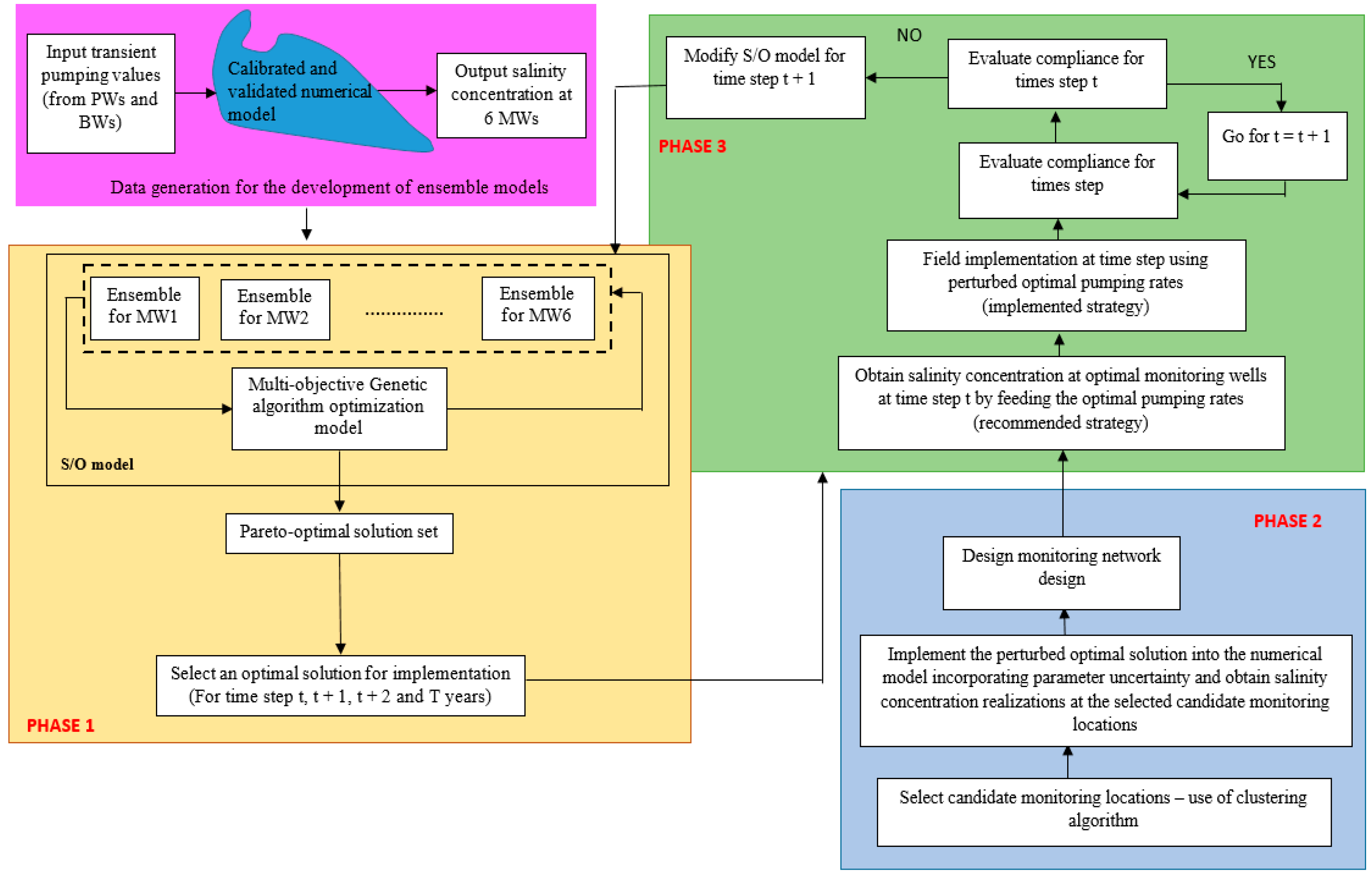
2.1. Phase 1: Prescription and Implementation of an Optimal Management Strategy
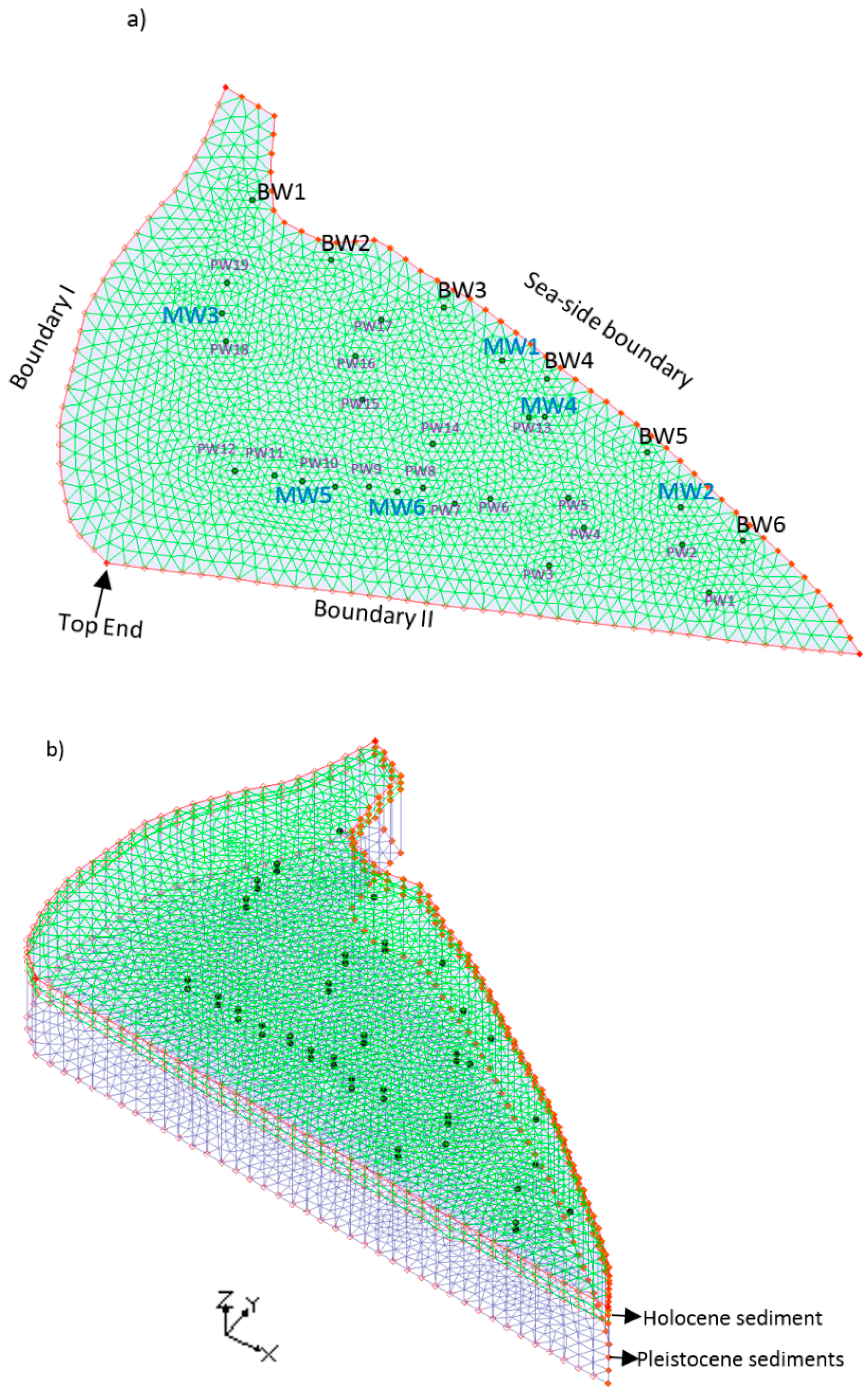
2.1.1. Numerical Groundwater Flow and Transport Model
2.1.2. Homogenous Support Vector Machine Regression-Based Ensemble Surrogate Models
2.1.3. Formulation of the Multi-Objective Coastal Aquifer Management Model
2.2. Phase 2: Regional-Scale Monitoring Network Design
2.2.1. Possible Deviations in Pumping and Aquifer Parameter Uncertainty
2.2.2. Location of Candidate Monitoring Wells
2.2.3. Formulation of the Optimal Monitoring Network Design Model
2.3. Phase 3: Sequential Modification of the Management Strategy
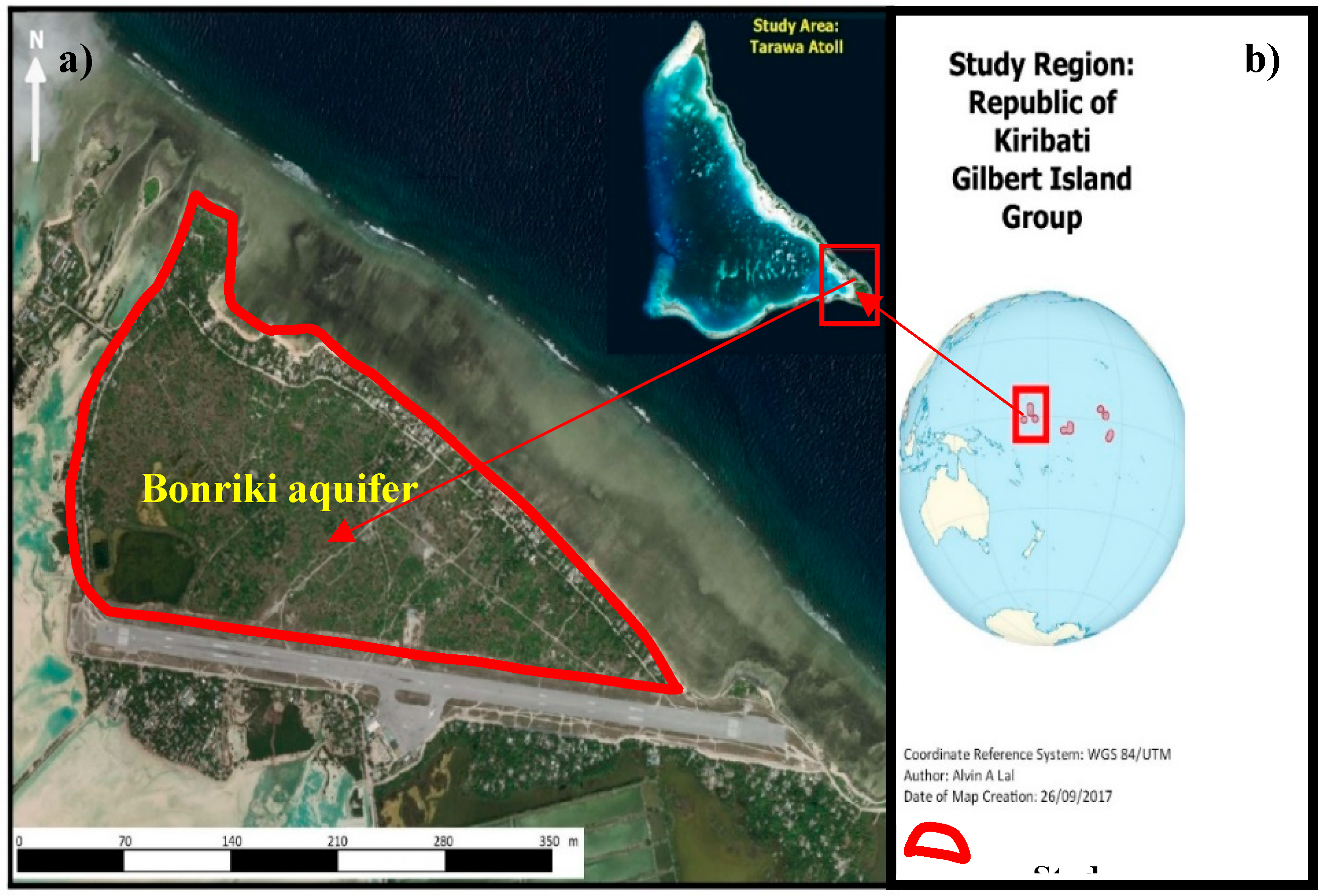
2.4. Case Study: Application and Evaluation of the Developed Methodology
3. Results and Discussions
3.1. Development and Execution of the Coupled S/O Model
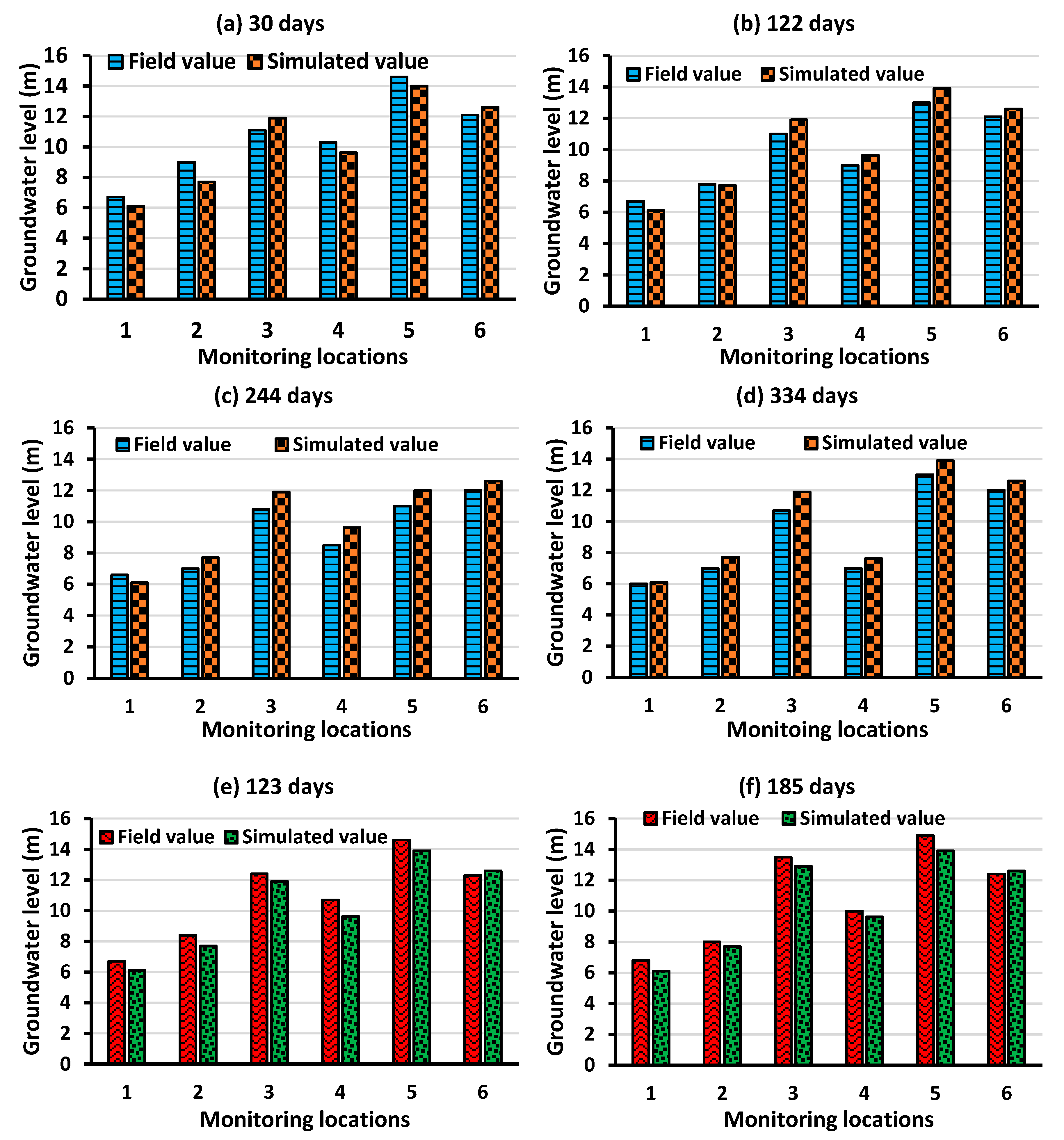
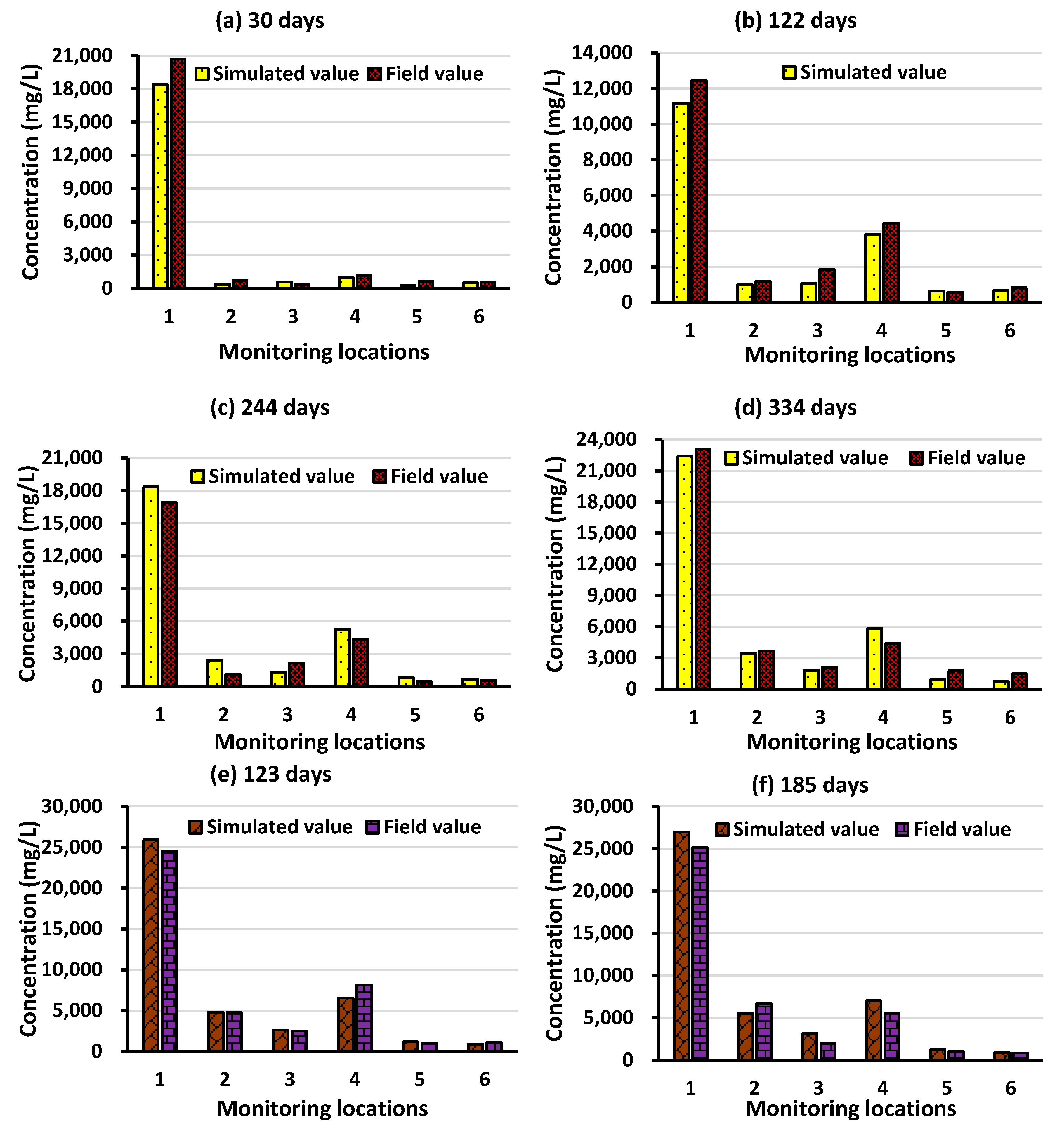
3.1.1. The Bonriki Aquifer Calibration and Validation Results
3.1.2. The Performance Evaluation of the Proposed Methodology Utilizing Homogenous Ensemble Models
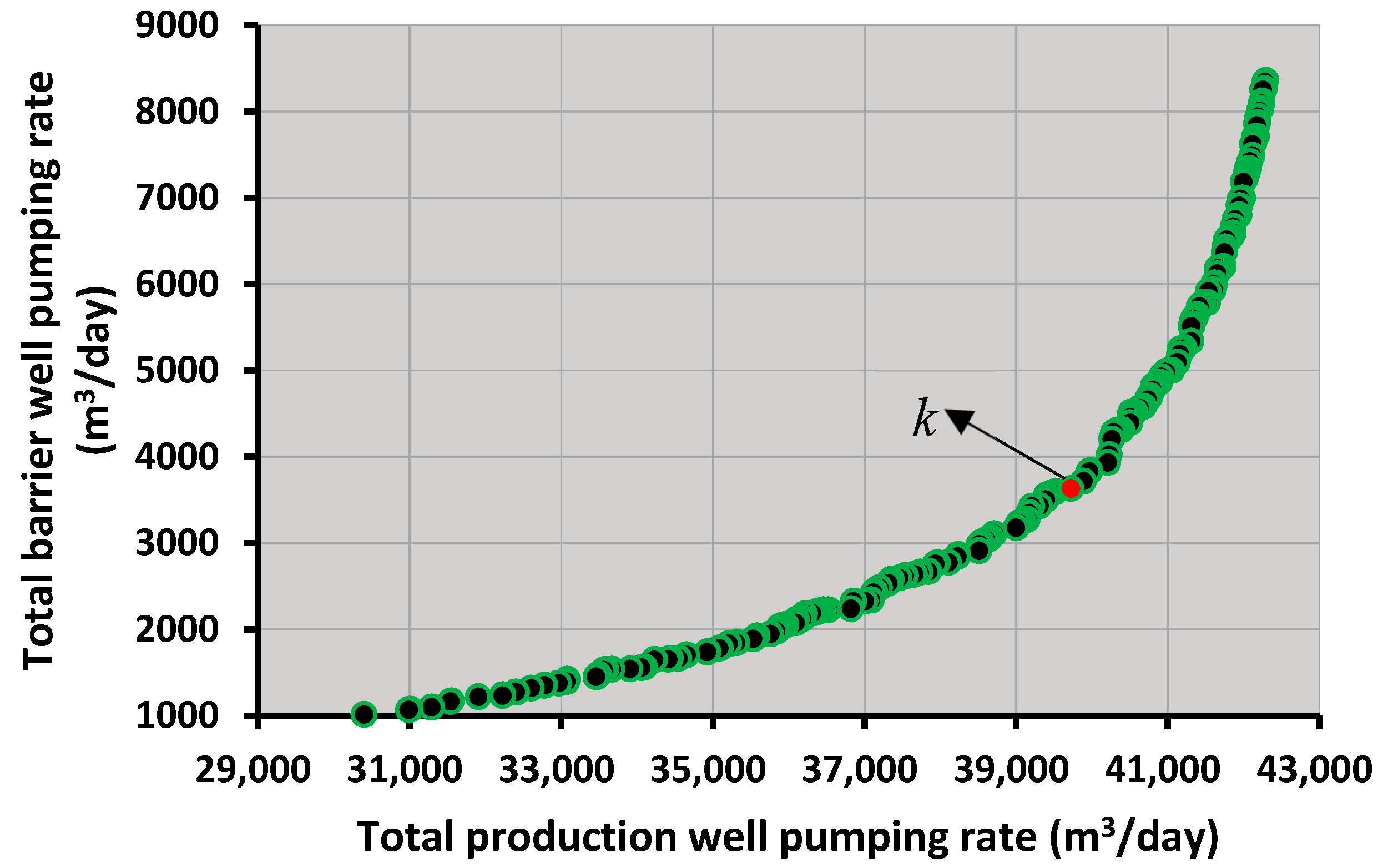
3.1.3. Implementation of the Optimal Aquifer Management Strategy
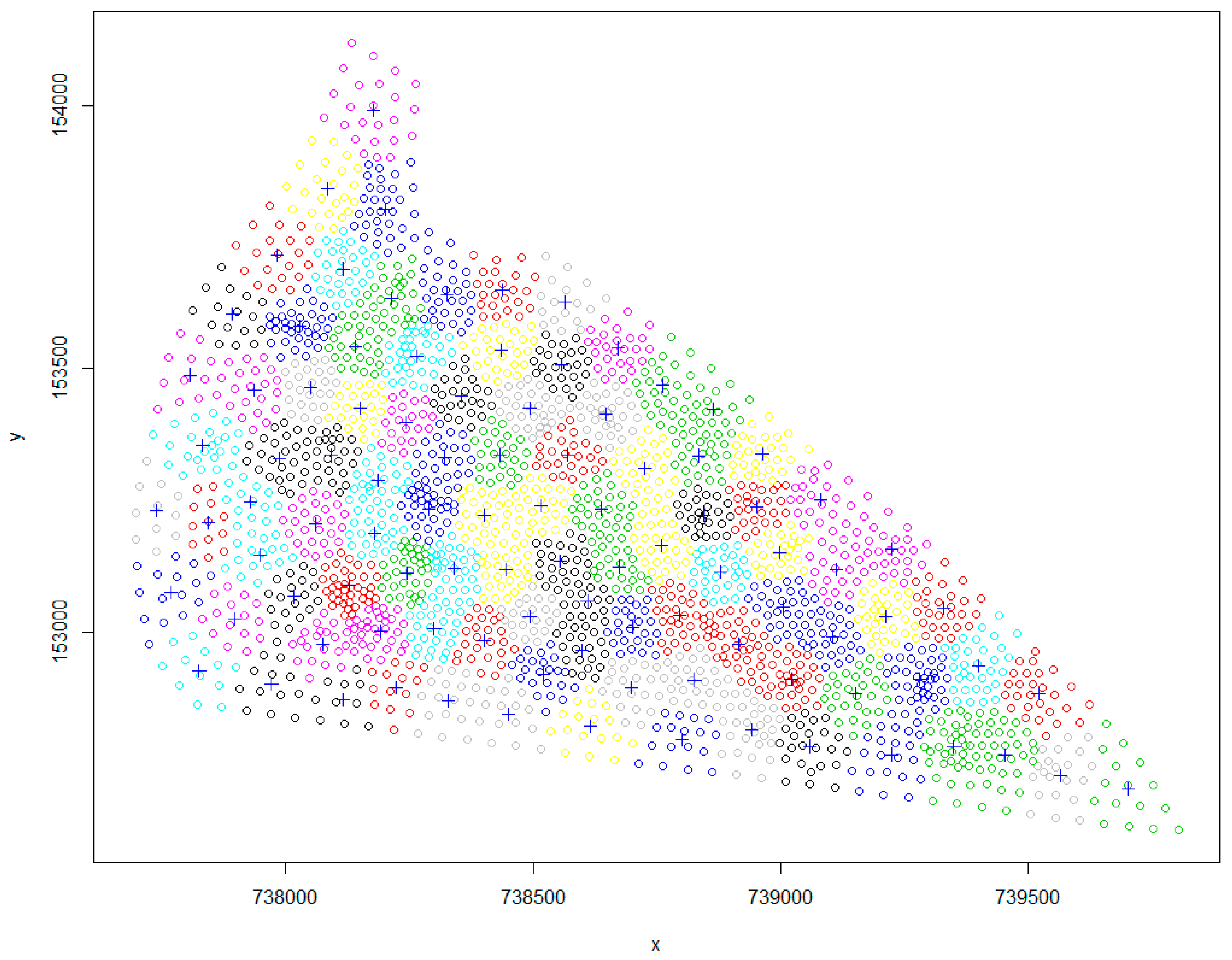
3.2. Optimal Monitoring Wells
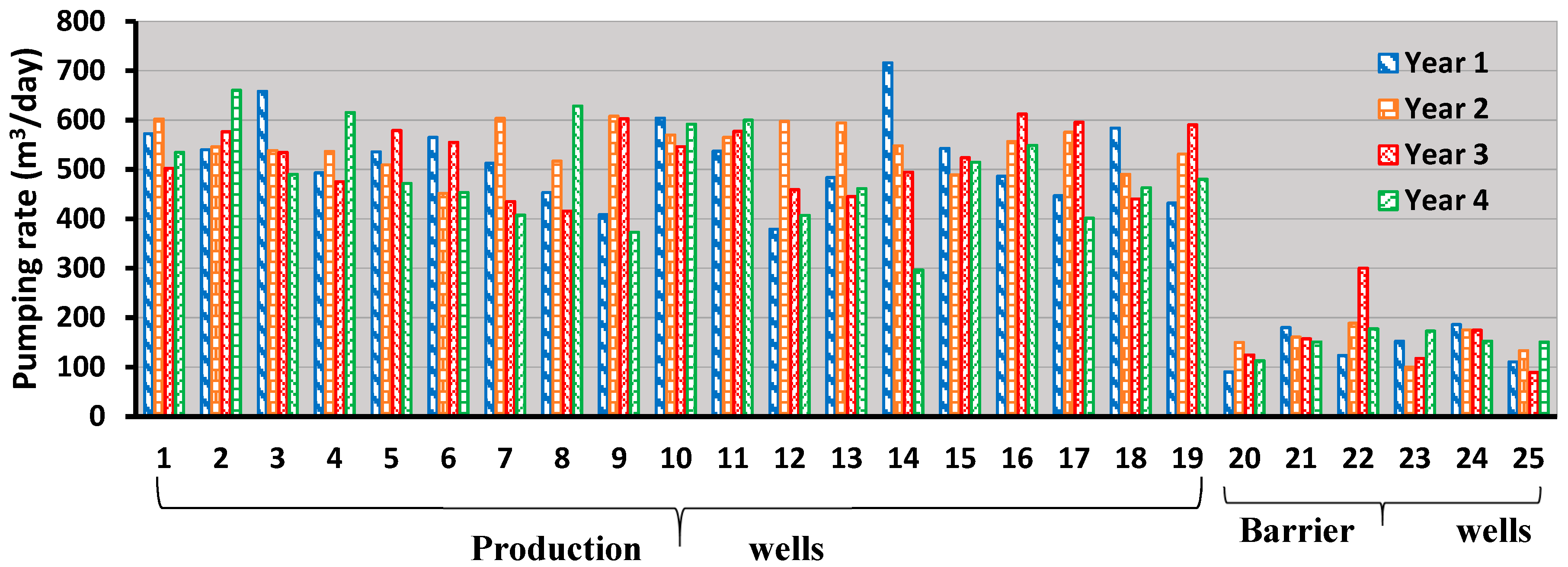
3.3. Modified Pumping Rates Using Feedback Information
4. Conclusions
Author Contributions
Funding
Acknowledgments
Conflicts of Interest
References
- Ahlfeld, D.P.; Barlow, P.M.; Mulligan, A.E. GWM–A Ground-Water Management Process for the US Geological Survey Modular Ground-Water Model (MODFLOW-2000); US Department of the Interior, US Geological Survey: Washington, DC, USA, 2005. [CrossRef]
- Ataie-Ashtiani, B.; Ketabchi, H.; Rajabi, M.M. Optimal management of a freshwater lens in a small island using surrogate models and evolutionary algorithms. J. Hydrol. Eng. 2013, 19, 339–354. [Google Scholar] [CrossRef]
- Ataie-Ashtiani, B.; Ketabchi, H. Elitist continuous ant colony optimization algorithm for optimal management of coastal aquifers. Water Resour. Manag. 2011, 25, 165–190. [Google Scholar] [CrossRef]
- Kourakos, G.; Mantoglou, A. Development of a multi-objective optimization algorithm using surrogate models for coastal aquifer management. J. Hydrol. 2013, 479, 13–23. [Google Scholar] [CrossRef]
- Park, N.; Shi, L. A comprehensive sharp-interface simulation-optimization model for fresh and saline groundwater management in coastal areas. Hydrogeol. J. 2015, 23, 1195–1204. [Google Scholar] [CrossRef]
- Dhar, A.; Datta, B. Saltwater intrusion management of coastal aquifers. I: Linked simulation-optimization. J. Hydrol. Eng. 2009, 14, 1263–1272. [Google Scholar] [CrossRef]
- Bhattacharjya, R.K.; Datta, B. Optimal Management of Coastal Aquifers Using Linked Simulation Optimization Approach. Water Resour. Manag. 2005, 19, 295–320. [Google Scholar] [CrossRef]
- Mantoglou, A.; Papantoniou, M. Optimal design of pumping networks in coastal aquifers using sharp interface models. J. Hydrol. 2008, 361, 52–63. [Google Scholar] [CrossRef]
- Das, A.; Datta, B. Development of multiobjective management models for coastal aquifers. J. Water Resour. Plan. Manag. 1999, 125, 76–87. [Google Scholar] [CrossRef]
- Sreekanth, J.; Datta, B. Multi-objective management of saltwater intrusion in coastal aquifers using genetic programming and modular neural network based surrogate models. J. Hydrol. 2010, 393, 245–256. [Google Scholar] [CrossRef]
- Roy, D.K.; Datta, B. A surrogate based multi-objective management model to control saltwater intrusion in multi-layered coastal aquifer systems. Civ. Eng. Environ. Syst. 2018, 34, 238–263. [Google Scholar] [CrossRef]
- Lal, A.; Datta, B. Modelling saltwater intrusion processes and development of a multi-objective strategy for management of coastal aquifers utilizing planned artificial freshwater recharge. Model. Earth Syst. Environ. 2017, 4, 111–126. [Google Scholar] [CrossRef]
- Lal, A.; Datta, B. Multiple objective management strategies for coastal aquifers utilizing new surrogate models. Int. J. Geomate 2018, 15, 79–85. [Google Scholar] [CrossRef]
- Lal, A.; Datta, B. Optimal Groundwater-Use Strategy for Saltwater Intrusion Management in a Pacific Island Country. J. Water Resour. Plan. Manag. 2019, 145, 04019032. [Google Scholar] [CrossRef]
- Sreekanth, J.; Datta, B. Coupled simulation-optimization model for coastal aquifer management using genetic programming-based ensemble surrogate models and multiple-realization optimization. Water Resour. Res. 2011, 47. [Google Scholar] [CrossRef]
- Roy, D.K.; Datta, B. Multivariate Adaptive Regression Spline Ensembles for Management of Multilayered Coastal Aquifers. J. Hydrol. Eng. 2017, 22, 04017031. [Google Scholar] [CrossRef]
- Lal, A.; Datta, B. Multi-objective groundwater management strategy under uncertainties for sustainable control of saltwater intrusion: Solution for an island country in the South Pacific. J. Environ. Manag. 2019, 234, 115–130. [Google Scholar] [CrossRef]
- Zhou, Y. Objectives, criteria and methodologies for the design of primary groundwater monitoring networks. IAHS Publ. Ser. Proc. Rep. Intern Assoc. Hydrol. Sci. 1994, 222, 285–296. [Google Scholar]
- Zhou, Y.; Dong, D.; Liu, J.; Li, W. Upgrading a regional groundwater level monitoring network for Beijing Plain, China. Geosci. Front. 2013, 4, 127–138. [Google Scholar] [CrossRef]
- Yang, F.-g.; Cao, S.-y.; Liu, X.-n.; Yang, K.-j. Design of groundwater level monitoring network with ordinary kriging. J. Hydrodyn. 2008, 20, 339–346. [Google Scholar] [CrossRef]
- Kumar, S.; Sondhi, S.; Phogat, V. Network design for groundwater level monitoring in upper Bari Doab canal tract, Punjab, India. Irrig. Drain. J. Int. Comm. Irrig. Drain. 2005, 54, 431–442. [Google Scholar] [CrossRef]
- Prinos, S.T.; Lietz, A.; Irvin, R. Design of a Real-Time Ground-Water Level Monitoring Network and Portrayal of Hydrologic Data in Southern Florida; Geological Survey: Preston, UK, 2002. [CrossRef]
- Meyer, P.D.; Valocchi, A.J.; Eheart, J.W. Monitoring network design to provide initial detection of groundwater contamination. Water Resour. Res. 1994, 30, 2647–2659. [Google Scholar] [CrossRef]
- Dhar, A.; Datta, B. Multiobjective design of dynamic monitoring networks for detection of groundwater pollution. J. Water Resour. Plan. Manag. 2007, 133, 329–338. [Google Scholar] [CrossRef]
- Storck, P.; Eheart, J.W.; Valocchi, A.J. A method for the optimal location of monitoring wells for detection of groundwater contamination in three-dimensional heterogenous aquifers. Water Resour. Res. 1997, 33, 2081–2088. [Google Scholar] [CrossRef]
- Mahar, P.S.; Datta, B. Optimal monitoring network and ground-water–pollution source identification. J. Water Resour. Plan. Manag. 1997, 123, 199–207. [Google Scholar] [CrossRef]
- Prakash, O.; Datta, B. Sequential optimal monitoring network design and iterative spatial estimation of pollutant concentration for identification of unknown groundwater pollution source locations. Environ. Monit. Assess. 2013, 185, 5611–5626. [Google Scholar] [CrossRef]
- Hudak, P.F.; Loaiciga, H.A. A location modeling approach for groundwater monitoring network augmentation. Water Resour. Res. 1992, 28, 643–649. [Google Scholar] [CrossRef]
- Zhu, X.; Yue, Y.; Wong, P.W.; Zhang, Y.; Ding, H. Designing an Optimized Water Quality Monitoring Network with Reserved Monitoring Locations. Water 2019, 11, 713. [Google Scholar] [CrossRef]
- Baalousha, H. Assessment of a groundwater quality monitoring network using vulnerability mapping and geostatistics: A case study from Heretaunga Plains, New Zealand. Agric. Water Manag. 2010, 97, 240–246. [Google Scholar] [CrossRef]
- Mogheir, Y.; Singh, V. Application of information theory to groundwater quality monitoring networks. Water Resour. Manag. 2002, 16, 37–49. [Google Scholar] [CrossRef]
- Masoumi, F.; Kerachian, R. Optimal redesign of groundwater quality monitoring networks: A case study. Environmental Monit. Assess. 2010, 161, 247–257. [Google Scholar] [CrossRef]
- Ammar, K.; Khalil, A.; McKee, M.; Kaluarachchi, J. Bayesian deduction for redundancy detection in groundwater quality monitoring networks. Water Resour. Res. 2008, 44. [Google Scholar] [CrossRef]
- Loaiciga, H.A. An optimization approach for groundwater quality monitoring network design. Water Resour. Res. 1989, 25, 1771–1782. [Google Scholar] [CrossRef]
- Zhang, Y.; Pinder, G.F.; Herrera, G.S. Least cost design of groundwater quality monitoring networks. Water Resour. Res. 2005, 41. [Google Scholar] [CrossRef]
- Reed, P.; Minsker, B.; Valocchi, A.J. Cost-effective long-term groundwater monitoring design using a genetic algorithm and global mass interpolation. Water Resour. Res. 2000, 36, 3731–3741. [Google Scholar] [CrossRef]
- Destandau, F.; Zaiter, Y. Optimal spatio-temporal design for water quality monitoring networks in maximizing economic value of information. In Proceedings of the MATEC Web of Conferences; EDP Sciences: Les Ulis, France, 2019; p. 03004. [Google Scholar] [CrossRef]
- Loaiciga, H.A.; Charbeneau, R.J.; Everett, L.G.; Fogg, G.E.; Hobbs, B.F.; Rouhani, S. Review of ground-water quality monitoring network design. J. Hydraul. Eng. 1992, 118, 11–37. [Google Scholar] [CrossRef]
- Sreekanth, J.; Datta, B. Design of an optimal compliance monitoring network and feedback information for adaptive management of saltwater intrusion in coastal aquifers. J. Water Resour. Plan. Manag. 2013, 140, 04014026. [Google Scholar] [CrossRef]
- Dhar, A.; Datta, B. Saltwater intrusion management of coastal aquifers. II: Operation uncertainty and monitoring. J. Hydrol. Eng. 2009, 14, 1273–1282. [Google Scholar] [CrossRef]
- Žalik, K.R. An efficient k′-means clustering algorithm. Pattern Recognit. Lett. 2008, 29, 1385–1391. [Google Scholar] [CrossRef]
- Bandyopadhyay, S.; Maulik, U. An evolutionary technique based on K-means algorithm for optimal clustering in RN. Inf. Sci. 2002, 146, 221–237. [Google Scholar] [CrossRef]
- Nazeer, K.A.; Sebastian, M. Improving the Accuracy and Efficiency of the k-means Clustering Algorithm. In Proceedings of the World Congress on Engineering, London, UK, 3–5 July 2009; pp. 1–3. [Google Scholar]
- Post, V.E.; Bosserelle, A.L.; Galvis, S.C.; Sinclair, P.J.; Werner, A.D. On the resilience of small-island freshwater lenses: Evidence of the long-term impacts of groundwater abstraction on Bonriki Island, Kiribati. J. Hydrol. 2018, 564, 133–148. [Google Scholar] [CrossRef]
- Lin, H.-C.J.; Richards, D.R.; Yeh, G.-T.; Cheng, J.-R.; Cheng, H.-P. FEMWATER: A Three-Dimensional Finite Element Computer Model for Simulating Density-Dependent Flow and Transport in Variably Saturated Media; CHL-97-12; DTIC Document: Vicksburg, MS, USA, 1997. [Google Scholar]
- Roy, D.K.; Datta, B. Fuzzy C-Mean Clustering Based Inference System for Saltwater Intrusion Processes Prediction in Coastal Aquifers. Water Resour. Manag. 2016, 31, 1–22. [Google Scholar] [CrossRef]
- Lal, A.; Datta, B. Development and Implementation of Support Vector Machine Regression Surrogate Models for Predicting Groundwater Pumping-Induced Saltwater Intrusion into Coastal Aquifers. Water Resour. Manag. 2018, 32, 1–15. [Google Scholar] [CrossRef]
- Liu, J.; Zio, E. An adaptive online learning approach for Support Vector Regression: Online-SVR-FID. Mech. Syst. Signal Process. 2016, 76, 796–809. [Google Scholar] [CrossRef]
- Shu, C.; Burn, D.H. Artificial neural network ensembles and their application in pooled flood frequency analysis. Water Resour. Res. 2004, 40. [Google Scholar] [CrossRef]
- Perrone, M.P.; Cooper, L.N. When networks disagree: Ensemble methods for hybrid neural networks. In How We Learn; How We Remember: Toward An Understanding Of Brain And Neural Systems: Selected Papers of Leon N Cooper; World Scientific: Singapore, 1995; pp. 342–358. [Google Scholar] [CrossRef]
- Bishop, C.M. Neural Networks for Pattern Recognition; Oxford University Press: Oxford, UK, 1995. [Google Scholar]
- MacQueen, J. Some methods for classification and analysis of multivariate observations. In Proceedings of the Fifth Berkeley Symposium on Mathematical Statistics and Probability, Oakland, CA, USA, 7 January 1967; pp. 281–297. [Google Scholar]
- Dhar, A.; Datta, B. Logic-based design of groundwater monitoring network for redundancy reduction. J. Water Resour. Plan. Manag. 2009, 136, 88–94. [Google Scholar] [CrossRef]
- White, I.; Falkland, T.; Crennan, L.; Jones, P.; Metutera, T.; Etuati, B.; Metai, E. Groundwater recharge in low coral island Bonriki, South Tarawa, Republic of Kiribati: Isues, traditions and conflicts in groundwater use and management. In Technical Documents in Hydrology; UNESCO: Paris, France, 1999; Volume 25. [Google Scholar]
- Metutera, T. Water management in Kiribati with special emphasis on groundwater development using infiltration galleries. In Proceedings of the Pacific Regional Consultation on Water in Small Island Countries, Sigatoka, Fiji, 29 July 2002; p. 29. [Google Scholar]
- Bosserelle, A.; Jakovovic, D.; Post, V.; Rodriguez, S.G.; Werner, A.; Sinclair, P. Bonriki Inundation Vulnerability Assessment (BIVA): Assessment of Sea-Level Rise and Inundation Effects on Bonriki Freshwater Lens, Tarawa Kiribati-Groundwater Modelling report; SPC00010; Secretariat of the Pacific Community (SPC): Suva, Fiji, 2015. [Google Scholar]
- Bailey, R.T.; Jenson, J.; Olsen, A. Numerical modeling of atoll island hydrogeology. Groundwater 2009, 47, 184–196. [Google Scholar] [CrossRef]
- Sinclair, P.; Singh, A.; Leze, J.; Bosserelle, A.; Loco, A.; Mataio, M.; Bwatio, E.; Rodriguez, S.G. Bonriki Inundation Vulnerability Assessment: Groundwater Field Investigations Bonriki Water Reserve, South Tarawa, Kiribati; SPC00009; Secretariat of the Pacific Community (SPC): Suva, Fiji, 2015. [Google Scholar]
- Ghassemi, F.; Jakeman, A.; Jacobson, G. Mathematical modelling of sea water intrusion, Nauru Island. Hydrol. Process. 1990, 4, 269–281. [Google Scholar] [CrossRef]
- Ghassemi, F.; Jakeman, A.; Jacobson, G.; Howard, K. Simulation of seawater intrusion with 2D and 3D models: Nauru Island case study. Hydrogeol. J. 1996, 4, 4–22. [Google Scholar] [CrossRef]
- White, I.; Falkland, T.; Metutera, T.; Metai, E.; Overmars, M.; Perez, P.; Dray, A. Climatic and human influences on groundwater in low atolls. Vadose Zone J. 2007, 6, 581–590. [Google Scholar] [CrossRef]
- Underwood, M.R.; Peterson, F.L.; Voss, C.I. Groundwater lens dynamics of atoll islands. Water Resour. Res. 1992, 28, 2889–2902. [Google Scholar] [CrossRef]
- Oberdorfer, J.A.; Hogan, P.J.; Buddemeier, R.W. Atoll island hydrogeology: Flow and freshwater occurrence in a tidally dominated system. J. Hydrol. 1990, 120, 327–340. [Google Scholar] [CrossRef]
- Scharage, L. Optimization Modeling with LINGO; LINDO Systems, Inc.: Chicago, IL, USA, 1999. [Google Scholar]


| Parameter | Values | Source | ||
|---|---|---|---|---|
| Layer 1 | Layer 2 | |||
| Hydraulic conductivity (m/day) | x | 15 | 450 | calibrated |
| y | 7.5 | 225 | ||
| z | 1.5 | 45 | ||
| Porosity | 0.2 | 0.3 | calibrated | |
| Recharge | 0.0055 | calibrated | ||
| Seawater density (kg/m3) | 1025 | Oberdorfer et al. [63] | ||
| Freshwater density (kg/m3) | 1000 | Oberdorfer, Hogan, and Buddemeier [63] | ||
| Molecular diffusivity (m2/s) | 1.5 × 10⁻⁹ | Ghassemi, Jakeman, Jacobson, and Howard [60] | ||
| Dynamic viscosity of water (kg/ms) | 280,985.8 | - | ||
| Longitudinal dispersivity (m) | 1 | Bosserelle, Jakovovic, Post, Rodriguez, Werner, and Sinclair [56] | ||
| Lateral dispersivity (m) | 0.05 | Bosserelle, Jakovovic, Post, Rodriguez, Werner, and Sinclair [56] | ||
| Compressibility of water (m2/N) | 4.4 × 10⁻¹⁰ | Oberdorfer, Hogan, and Buddemeier [63] | ||
| Model | Evaluation Criteria | SVMR1 | SVMR2 | SVMR3 | SVMR4 | SVMR5 | SVMR6 |
|---|---|---|---|---|---|---|---|
| NM1 | RMSE | 5.10 | 6.17 | 3.74 | 2.95 | 2.02 | 1.89 |
| MBE | 0.41 | 0.45 | 0.38 | 0.41 | 0.39 | 0.35 | |
| r | 0.96 | 0.97 | 0.97 | 0.97 | 0.98 | 0.98 | |
| NSE | 0.97 | 0.96 | 0.98 | 0.97 | 0.98 | 0.98 | |
| IOA | 0.94 | 0.95 | 0.95 | 0.96 | 0.96 | 0.96 | |
| NM2 | RMSE | 5.98 | 5.62 | 2.82 | 2.04 | 1.59 | 1.33 |
| MBE | 0.47 | 0.56 | 0.62 | 0.52 | 0.39 | 0.44 | |
| r | 0.97 | 0.97 | 0.98 | 0.97 | 0.98 | 0.98 | |
| NSE | 0.96 | 0.96 | 0.96 | 0.97 | 0.97 | 0.97 | |
| IOA | 0.95 | 0.94 | 0.95 | 0.96 | 0.96 | 0.96 | |
| NM3 | RMSE | 4.16 | 5.22 | 3.51 | 4.86 | 3.02 | 2.14 |
| MBE | 0.71 | 0.43 | 0.48 | 0.47 | 0.38 | 0.31 | |
| r | 0.97 | 0.96 | 0.97 | 0.96 | 0.98 | 0.98 | |
| NSE | 0.97 | 0.97 | 0.98 | 0.97 | 0.98 | 0.99 | |
| IOA | 0.94 | 0.95 | 0.95 | 0.94 | 0.95 | 0.96 | |
| NM4 | RMSE | 6.60 | 5.33 | 5.27 | 4.65 | 3.53 | 3.05 |
| MBE | 0.52 | 0.55 | 0.64 | 0.64 | 0.43 | 0.48 | |
| r | 0.97 | 0.98 | 0.96 | 0.97 | 0.97 | 0.97 | |
| NSE | 0.97 | 0.96 | 0.96 | 0.97 | 0.97 | 0.98 | |
| IOA | 0.95 | 0.94 | 0.93 | 0.95 | 0.95 | 0.96 | |
| NM5 | RMSE | 6.96 | 7.13 | 5.12 | 5.68 | 4.25 | 4.56 |
| MBE | 0.59 | 0.63 | 0.72 | 0.52 | 0.33 | 0.36 | |
| r | 0.97 | 0.97 | 0.97 | 0.97 | 0.98 | 0.97 | |
| NSE | 0.97 | 0.98 | 0.98 | 0.97 | 0.98 | 0.97 | |
| IOA | 0.95 | 0.94 | 0.95 | 0.94 | 0.96 | 0.95 | |
| NM6 | RMSE | 7.63 | 5.32 | 5.24 | 5.69 | 4.25 | 3.57 |
| MBE | 0.44 | 0.65 | 0.66 | 0.46 | 0.41 | 0.34 | |
| r | 0.97 | 0.98 | 0.98 | 0.97 | 0.99 | 0.99 | |
| NSE | 0.98 | 0.98 | 0.98 | 0.98 | 0.98 | 0.99 | |
| IOA | 0.96 | 0.97 | 0.97 | 0.97 | 0.98 | 0.98 | |
| NM7 | RMSE | 7.26 | 6.75 | 6.03 | 5.87 | 5.66 | 5.12 |
| MBE | 0.58 | 0.62 | 0.55 | 0.47 | 0.44 | 0.36 | |
| r | 0.97 | 0.98 | 0.98 | 0.98 | 0.98 | 0.99 | |
| NSE | 0.97 | 0.98 | 0.98 | 0.98 | 0.98 | 0.99 | |
| IOA | 0.96 | 0.97 | 0.97 | 0.97 | 0.98 | 0.98 | |
| NM8 | RMSE | 6.35 | 7.16 | 5.57 | 5.31 | 5.26 | 5.19 |
| MBE | 0.54 | 0.58 | 0.52 | 0.49 | 0.33 | 0.41 | |
| r | 0.98 | 0.97 | 0.98 | 0.98 | 0.98 | 0.98 | |
| NSE | 0.97 | 0.97 | 0.97 | 0.97 | 0.97 | 0.97 | |
| IOA | 0.96 | 0.95 | 0.96 | 0.96 | 0.96 | 0.96 | |
| NM9 | RMSE | 7.37 | 6.89 | 8.43 | 6.22 | 5.32 | 4.41 |
| MBE | 0.59 | 0.63 | 0.67 | 0.56 | 0.42 | 0.38 | |
| r | 0.98 | 0.98 | 0.96 | 0.97 | 0.97 | 0.98 | |
| NSE | 0.97 | 0.97 | 0.96 | 0.97 | 0.97 | 0.98 | |
| IOA | 0.95 | 0.96 | 0.95 | 0.96 | 0.97 | 0.97 | |
| NM10 | RMSE | 7.14 | 6.59 | 6.91 | 5.88 | 4.71 | 4.28 |
| MBE | 0.55 | 0.62 | 0.52 | 0.55 | 0.39 | 0.44 | |
| r | 0.98 | 0.98 | 0.98 | 0.98 | 0.98 | 0.99 | |
| NSE | 0.98 | 0.98 | 0.98 | 0.98 | 0.98 | 0.99 | |
| IOA | 0.96 | 0.97 | 0.97 | 0.97 | 0.97 | 0.98 |
| Evaluation Criteria | En_SVMR1 | En_SVMR2 | En_SVMR3 | En_SVMR4 | En_SVMR5 | En_SVMR6 |
|---|---|---|---|---|---|---|
| RMSE | 4.70 | 5.61 | 3.34 | 2.99 | 2.16 | 1.79 |
| MBE | 0.42 | 0.44 | 0.36 | 0.41 | 0.33 | 0.31 |
| r | 0.97 | 0.97 | 0.98 | 0.97 | 0.98 | 0.98 |
| NSE | 0.98 | 0.97 | 0.98 | 0.98 | 0.98 | 0.98 |
| IOA | 0.96 | 0.96 | 0.96 | 0.97 | 0.97 | 0.97 |
| Solution Number | MW1 | MW2 | MW3 | MW4 | MW5 | MW6 | ||||||
|---|---|---|---|---|---|---|---|---|---|---|---|---|
| NMav (mg/L) | En_SVMR1 (mg/L) | NMav (mg/L) | En_SVMR2 (mg/L) | NMav (mg/L) | En_SVMR3 (mg/L) | NMav (mg/L) | En_SVMR4 (mg/L) | NMav (mg/L) | En_SVMR5 (mg/L) | NMav (mg/L) | En_SVMR6 (mg/L) | |
| 1 | 19,870.4 | 19,677.0 | 19,795.63 | 19,742.53 | 4868.18 | 4844.85 | 3963.43 | 3932.23 | 447.82 | 444.94 | 432.72 | 429.88 |
| 2 | 19,708.8 | 19,621.2 | 19,783.73 | 19,735.64 | 4811.80 | 4776.57 | 3959.52 | 3916.66 | 433.94 | 429.27 | 435.97 | 433.33 |
| 3 | 20,009.2 | 19,846.9 | 19,975.89 | 19,949.89 | 4931.85 | 4928.47 | 3944.47 | 3911.19 | 444.84 | 437.12 | 436.18 | 431.45 |
| 4 | 19,798.4 | 19,660.5 | 19,793.16 | 19,757.80 | 4915.77 | 4906.76 | 3868.29 | 3868.82 | 433.54 | 427.58 | 439.93 | 436.34 |
| 5 | 19,727.4 | 19,567.6 | 19,829.44 | 19,795.19 | 4828.40 | 4839.35 | 3972.34 | 3967.71 | 430.35 | 427.29 | 427.90 | 426.47 |
| Year 1 | Year 2 | Year 3 | Year 4 | |||||
|---|---|---|---|---|---|---|---|---|
| OMW | Situation A | Situation B | Situation A | Situation B | Situation A | Situation B | Situation A | Situation B |
| 1 | 24,168.1 | 24,135.2 | 25,951.3 | 25,612.3 | 27,952.7 | 27,956.3 | 30,215.3 | 30,258.1 |
| 2 | 23,256.9 | 23,247.7 | 24,696.1 | 24,616.6 | 26,151.9 | 26,146.5 | 27,298.6 | 27,204.7 |
| 3 | 23,055.8 | 23,016.3 | 24,856.2 | 24,843.2 | 25,871.4 | 25,886.9 | 26,598.3 | 26,577.2 |
| 4 | 24,136.8 | 24,089.6 | 24,623.6 | 24,647.9 | 25,027.0 | 25,049.7 | 26,884.3 | 26,813.6 |
| 5 | 17,452.3 | 17,486.3 | 17,898.2 | 17,954.6 | 19,560.1 | 19,587.8 | 22,389.7 | 22,384.0 |
| 6 | 19,585.6 | 19,546.2 | 20,115.0 | 20,168.8 | 22,895.4 | 22,905.7 | 25,468.9 | 25,424.0 |
| 7 | 23,657.0 | 23,641.3 | 24,891.3 | 24,923.6 | 26,454.7 | 26,484.7 | 28,355.8 | 28,397.1 |
| 8 | 24,556.3 | 24,587.3 | 25,831.3 | 25,838.5 | 27,206.8 | 27,198.2 | 28,114.0 | 28,046.8 |
| 9 | 23,584.0 | 23,547.0 | 24,669.3 | 24,646.9 | 26,158.3 | 26,144.3 | 27,138.2 | 27,138.2 |
| 10 | 25,136.6 | 25,136.2 | 26,882.2 | 26,876.3 | 28,654.2 | 28,679.3 | 30,219.0 | 30,158.5 |
| Year 1 | Year 2 | Year 3 | Year 4 | |||||
|---|---|---|---|---|---|---|---|---|
| R | I | R | I | R | I | R | I | |
| Year 1 | 9946.9 | 9822.6 | ||||||
| Year 2 | 10,426.5 | 10,335.1 | 10,378.8 | |||||
| Year 3 | 9957.6 | 9987.1 | 9874.2 | 9904.4 | ||||
| Year 4 | 9397.5 | 9414.9 | 9369.2 | 9325.3 | - | |||
| Total | 39,728.4 | 29,737.1 | 19,243.4 | 9325.3 | ||||
© 2019 by the authors. Licensee MDPI, Basel, Switzerland. This article is an open access article distributed under the terms and conditions of the Creative Commons Attribution (CC BY) license (http://creativecommons.org/licenses/by/4.0/).
Share and Cite
Lal, A.; Datta, B. Application of Monitoring Network Design and Feedback Information for Adaptive Management of Coastal Groundwater Resources. Int. J. Environ. Res. Public Health 2019, 16, 4365. https://doi.org/10.3390/ijerph16224365
Lal A, Datta B. Application of Monitoring Network Design and Feedback Information for Adaptive Management of Coastal Groundwater Resources. International Journal of Environmental Research and Public Health. 2019; 16(22):4365. https://doi.org/10.3390/ijerph16224365
Chicago/Turabian StyleLal, Alvin, and Bithin Datta. 2019. "Application of Monitoring Network Design and Feedback Information for Adaptive Management of Coastal Groundwater Resources" International Journal of Environmental Research and Public Health 16, no. 22: 4365. https://doi.org/10.3390/ijerph16224365
APA StyleLal, A., & Datta, B. (2019). Application of Monitoring Network Design and Feedback Information for Adaptive Management of Coastal Groundwater Resources. International Journal of Environmental Research and Public Health, 16(22), 4365. https://doi.org/10.3390/ijerph16224365