Spatiotemporal Associations between PM_2.5 and SO₂ as well as NO₂ in China from 2015 to 2018

Abstract

Given the critical roles of nitrates and sulfates in fine particulate matter (PM_2.5) formation, we examined spatiotemporal associations between PM_2.5 and sulfur dioxide (SO₂) as well as nitrogen dioxide (NO₂) in China by taking advantage of the in situ observations of these three pollutants measured from the China national air quality monitoring network for the period from 2015 to 2018. Maximum covariance analysis (MCA) was applied to explore their possible coupled modes in space and time. The relative contribution of SO₂ and NO₂ to PM_2.5 was then quantified via a statistical modeling scheme. The linear trends derived from the stratified data show that both PM_2.5 and SO₂ decreased significantly in northern China in terms of large values, indicating a fast reduction of high PM_2.5 and SO₂ loadings therein. The statistically significant coupled MCA mode between PM_2.5 and SO₂ indicated a possible spatiotemporal linkage between them in northern China, especially over the Beijing–Tianjin–Hebei region. Further statistical modeling practices revealed that the observed PM_2.5 variations in northern China could be explained largely by SO₂ rather than NO₂ therein, given the estimated relatively high importance of SO₂. In general, the evidence-based results in this study indicate a strong linkage between PM_2.5 and SO₂ in northern China in the past few years, which may help to better investigate the mechanisms behind severe haze pollution events in northern China.

1. Introduction

Concentrations of fine particulate matter (denoted as PM_2.5) in China have decreased prominently during the time period of 2013–2018 due to the implementation of the air pollution prevention and control action plan [1,2,3]. Further investigations indicate that the observed reduction of PM_2.5 loadings in China could be largely attributed to the implementation of many effective air pollution control policies, such as fuel quality promotion and usage of cleaner energy, and especially the reduction of industrial emissions of air pollutants like sulfates and nitrogen oxides [4,5,6].

Many previous studies have evaluated the spatial and temporal variations of PM_2.5 concentrations in China in terms of either trend estimation or spatial clustering analysis. For instance, using a global and local Moran’s I index, Ye et al. (2018) [7] examined the spatiotemporal patterns of PM_2.5 in 338 major Chinese cities at multiple time-scales, and found that PM_2.5 in China has evident spatial autocorrelation and clustering characteristics with “hot spots” identified in the Beijing–Tianjin–Hebei (BTH) region and southwest Xinjiang. By taking advantage of satellite-based PM_2.5 estimations, Ma et al. (2015) [8] analyzed the spatiotemporal trends of PM_2.5 nationwide and found that PM_2.5 in China increased during 2004 to 2007, and has decreased since then. Similar effects were also revealed in Reference [1], but with more spatial details, as the PM_2.5 inflection time was identified at each grid pixel. Moreover, their results indicate that performing trend analysis on stratified data (e.g., large values) is more informative and meaningful for evaluating the effectiveness of emission control actions on PM_2.5 pollution levels [1].

Aside from trend analysis, correlations between PM_2.5 and other air pollutants such as nitrogen dioxide (NO₂), sulfur dioxide (SO₂), carbon monoxide, and ozone have also been examined in many studies [4,9], aiming to explore their possible interactions in space and time [10]. Due to complex mechanisms of PM_2.5 formation and variation, attribution of the observed PM_2.5 variations to precursor gases via correlation analysis is by no means an easy task. Numerical simulations are always needed to achieve such a goal via sensitivity experiments, by considering various influential factors such as anthropogenic emissions and meteorological conditions [3,11,12,13,14].

Previous studies have revealed that anthropogenic emissions of SO₂ and NO₂ play important roles in the process of secondary fine particulate matter formation [6,15,16]. Although the newly established China national ambient air quality monitoring work has provided ample first-hand observations of six essential air pollutants on an hourly basis since 2013, few studies have attempted to examine the possible spatiotemporal associations between PM_2.5 and SO₂ as well as NO₂ at the national scale using these valuable long-term in situ records.

In this study, ground measured concentrations of PM_2.5 and SO₂ as well as NO₂ in China from 2015 to 2018 were used to explore possible associations between them in space and time. Differing from previous correlation analysis, maximum covariance analysis (MCA) was applied here to identify possible coupled spatiotemporal modes between PM_2.5 and the other two pollutants. Statistical modeling practices were subsequently performed to explore the statistical relationship between them, aiming to resolve the relative contribution of SO₂ and NO₂ to the observed PM_2.5 variations. Science questions to be answered by this study may include: (1) Is there any statistically significant association between PM_2.5 and SO₂ and/or NO₂ in space and time across China? (2) To what extent can the observed PM_2.5 variations be explained by SO₂ and NO₂? (3) Which factor is more important in modulating the observed PM_2.5 variations?

2. Materials and Methods

2.1. Data Sources

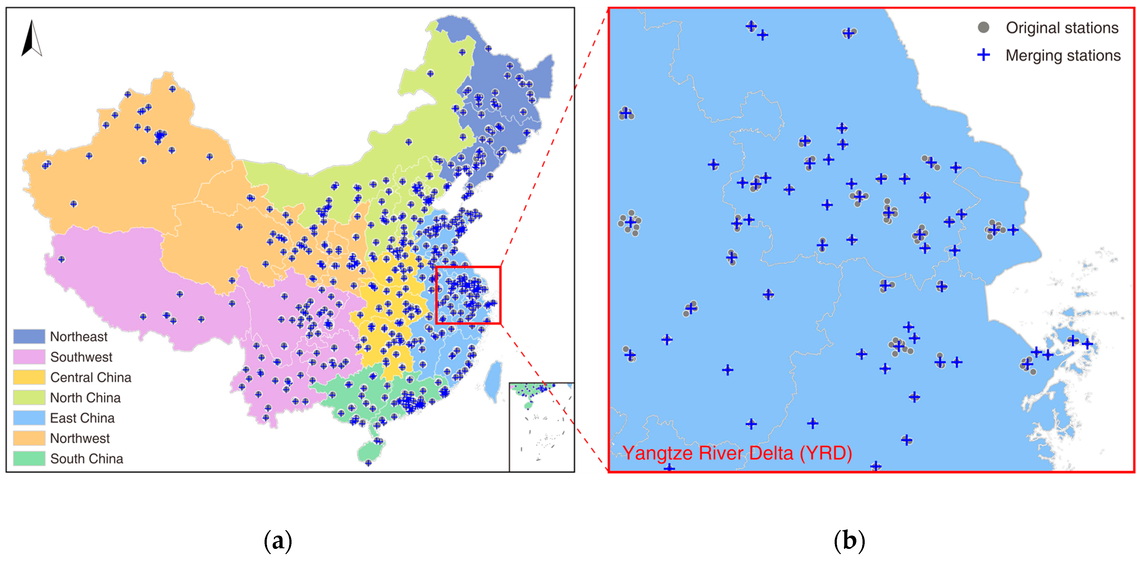
2.1.1. In Situ Air Quality Records

Hourly PM_2.5, SO₂, and NO₂ concentration records during the period of 1 January 2015 to 31 December 2018, acquired from the China national environmental monitoring center, were employed. China began establishing a national ambient air quality monitoring network in 2013. To date, more than 1600 state-level monitoring stations have been deployed across 338 major Chinese cities. The spatial distribution of these stations can be found in Figure 1. Most of these stations are located in the east and south of China, where dense populations are found. Six essential air quality indicators (PM_2.5, PM₁₀, O₃, CO, NO₂, SO₂) are automatically sampled at each station, primarily using a tapered element oscillating microbalance analyzer and/or beta-attenuation monitor, and are then released publicly online by the China Environment Monitoring Center on an hourly basis.

2.1.2. Quality Control and Data Integration

Given observations from dense stations would not only result in significant information redundancy, but might increase the computational complexity due to significant spatial heterogeneity of air quality observations, data from 1604 stations were integrated into 530 data sets via spatial hierarchy clustering by following the process as detailed in Reference [1]. As shown in Figure 1, the clustered stations consisted of 369 merged stations and 161 independent stations.

Prior to data integration, essential quality control measures were applied to raw observations at each station to detect and remove outliers. First, a reference time series was created among stations within the same cluster using the median values of data from original stations, and a data value was referred to as an outlier once it exceeded triple (six times for SO₂ because of large variation) the 24 h standard deviations from the reference time series. Second, gradient difference was calculated for the previously screened time series to further identify outliers. Specifically, the quadratic derivatives were calculated and data values were deemed outliers once the quadratic gradient values were not within the range of −100 to 100. Such a screening enabled identification of outliers overlooked in the previous step. Around 3.9% of PM_2.5 observations (2.9% for SO₂ and 5.1% for NO₂) were identified as outliers and then removed. Quality assured hourly data values in each cluster were then averaged on a semi-monthly basis to create new time series for each air pollutant. Such a data integration scheme not only improved the data completeness in the temporal domain, but reduced the overall dimensionality of data sources. Finally, 530 clustered stations were attained, and records from only 499 stations were used for the subsequent analysis, given the presence of salient data gaps in data records from other 31 stations.

2.2. Methods

2.2.1. MCA Method

MCA was developed to identify coupled modes between two geophysical fields by maximizing their covariance rather than correlation in the time–space domain [17,18]. Because of this unique capability, MCA has been widely applied to link two geophysical fields in time and space, especially for climate change detection and attribution, since MCA enables resolution of the coupled fields and their presentation in both spatial and temporal domains [19,20]. A detailed description of the MCA method can be found elsewhere [17].

In terms of the identified coupled modes, whether these modes are statistically meaningful is always a big concern in real practice. In this study, Monte Carlo simulations were conducted to test the statistical significance of each MCA mode by randomly permuting the time series of one field [18,21,22]. The derived MCA modes were deemed statistically significant once the actual statistics were greater than those of their random counterparts. Prior to MCA analysis, the seasonality (i.e., annual cycle) of each variable was first removed, and the goal was to avoid possible influence from local atmospheric dynamic related variations. Specifically, PM_2.5 values at each semi-month of the year for the whole study period were averaged and then removed from the original time series. Similar procedures were also applied for SO₂ and NO₂ data sets.

In principle, mapping the left and right MCA derived singular vectors geographically would reveal synergetic variations of both fields in the spatial domain. Given singular vectors always have different magnitudes, most studies have converted them to either homogeneous or heterogeneous correlation maps to better interpret the MCA results [17,23,24,25]. Homogeneous correlation maps represent the correlation values between the expansion coefficient of one field and the time series of the same field at each grid point, with another field for heterogeneous maps [26]. In this study, the spatial pattern of coupled modes were presented in the form of covariance maps, since they reveal the spatial localization of the co-varying part on each field [17,26,27].

2.2.2. Quantifying the Relative Contribution of NO₂ and SO₂ to PM_2.5 Variations

Although MCA enables resolution of the coupled patterns between PM_2.5 and another two fields, it is challenging to determine which field plays a more important role in contributing to the observed PM_2.5 variations. Statistical modeling practices were therefore performed in the present study in the form of multiple linear regression (MLR) to further evaluate the relative contribution of NO₂ and SO₂ to the detected regional PM_2.5 variations. Specifically, PM_2.5 variations and the corresponding NO₂ and SO₂ information were first extracted from the hot spot regions as identified in the MCA modes. Subsequently, the extracted PM_2.5 time series were used as the dependent variable and the extracted principal components of NO₂ and SO₂ over the selected hot spot regions were used as explanatory variables.

The variance inflation factor (VIF) was calculated between these regressors to examine the possible collinearity problem. A threshold of 10 (an empirical value that is widely used in the literature) was also used in this study to determine the possible collinearity [28]. Finally, the LMG method [29], an advanced technique to determine the relative importance of explanatory variables in a linear model, was also applied to assess the relative contribution of NO₂ and SO₂ to the observed PM_2.5 variations. A detailed description of the calculation process of the LMG measure can be found elsewhere [29].

3. Results and Discussion

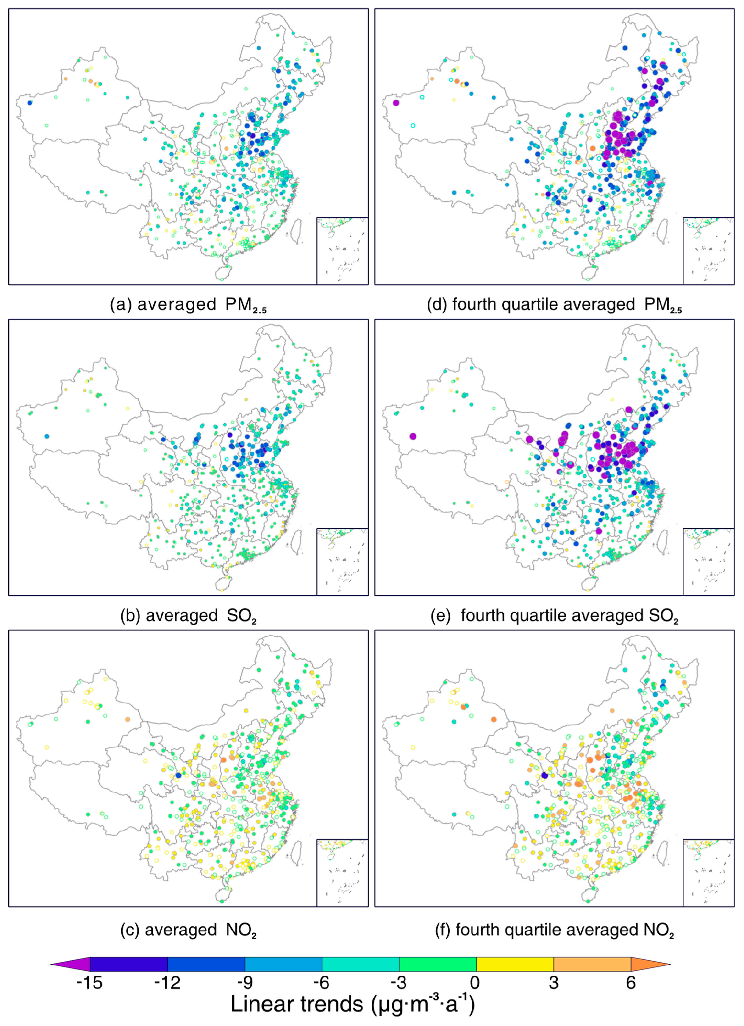
3.1. Linear Trends for PM_2.5 and SO₂ as well as NO₂

To better examine possible coupled spatiotemporal variations between PM_2.5 and SO₂ and NO₂, linear trends for each factor were firstly estimated using the least-square fitting method. Figure 2 shows the estimated linear trends for three factors between January 2015 and December 2018, and the left panel (Figure 2a–c) presents the trends estimated from an averaged value based on all data values, whereas the right counterparts (Figure 2d–f) were derived from their large values (i.e., averaged over values greater than the fourth quartile). It shows that PM_2.5 and SO₂ decreased markedly during the study time period, especially in northern China, where significant decreasing trends were observed. Moreover, in contrast to the trends estimated from all data value averages, trends estimated from large values were even more salient in northern China, indicating the effectiveness of clean air actions in reducing high loadings of PM_2.5 and SO₂ therein. However, no such significant declination effect was found for NO₂ concentrations across China. In contrast, marked increasing trends (dots shaded in orange) were even observed in some regions, for example over Shanxi and Anhui provinces.

Table 1. Region-specific linear trends (mean ± 95% confidence interval) for PM_2.5, SO₂, and NO₂ from 2015 to 2018. The unit of trend is μg/(m³·a). Numbers in brackets after division names are the total number of clustered stations in each division.

Divisions.	Averaged PM2.5 (Fourth Quartile Averaged)	Averaged SO2 (Fourth Quartile Averaged)	Averaged NO2 (Fourth Quartile Averaged)
Northeast (53)	−4.55 ± 2.02 (−8.86 ± 4.85)	−3.23 ± 1.06 (−6.21 ± 1.99)	−1.19 ± 0.77 (−1.72 ± 1.35)
North China (55)	−4.15 ± 2.48 (−8.47 ± 5.14)	−4.92 ± 1.69 (−9.35 ± 3.13)	−0.13 ± 1.07 (−0.01 ± 1.72)
Central China (56)	−4.81 ± 2.24 (−7.61 ± 3.96)	−4.07 ± 0.98 (−7.74 ± 1.71)	−0.45 ± 0.91 (−0.39 ± 1.50)
East China (139)	−3.69 ± 1.75 (−6.73 ± 3.27)	−3.78 ± 0.83 (−7.31 ± 1.52)	−0.41 ± 1.00 (−0.28 ± 1.72)
South China (64)	−1.07 ± 1.32 (−2.06 ± 2.28)	−0.84 ± 0.46 (−1.87 ± 0.87)	0.26 ± 0.82 (0.53 ± 1.46)
Northwest (73)	−1.47 ± 2.28 (−3.05 ± 4.54)	−2.37 ± 1.13 (−5.45 ± 2.24)	0.33 ± 0.95 (0.75 ± 1.53)
Southwest (59)	−2.19 ± 1.33 (−3.42 ± 2.20)	−1.40 ± 0.59 (−3.10 ± 1.08)	0.24 ± 0.70 (0.48 ± 1.17)

shows the estimated linear least-square trends for these three pollutants over seven major geographic divisions (refer to Figure 1 for the geolocation of these divisions) from 2015 to 2018. It is noticeable that concentrations of PM_2.5 and SO₂ decreased nationwide, but had different declining rates. In regard to PM_2.5, regions exhibiting the most significant decreasing trends included the northeast, northern China, and central China, by a rate of about −4 μg/(m³·a) for all value averaged concentrations and −8 μg/(m³·a) for large values. It shows that trends for large values almost doubled those of all value averaged concentrations, indicating the decline of PM_2.5 loading is mainly dominated by the decreasing of severe pollution episodes. A similar effect was also observed for SO₂, while northern China, central China, and east China were the three regions with the most significant declining trends. With respect to NO₂, both increasing and decreasing trends were observed, whereas most trends were statistically insignificant, except for the northeast, where NO₂ concentrations were observed with a statistically significant decreasing trend. These results collectively indicate that new actions should be implemented to control NO₂ emissions, toward the improvement of air quality nationwide.

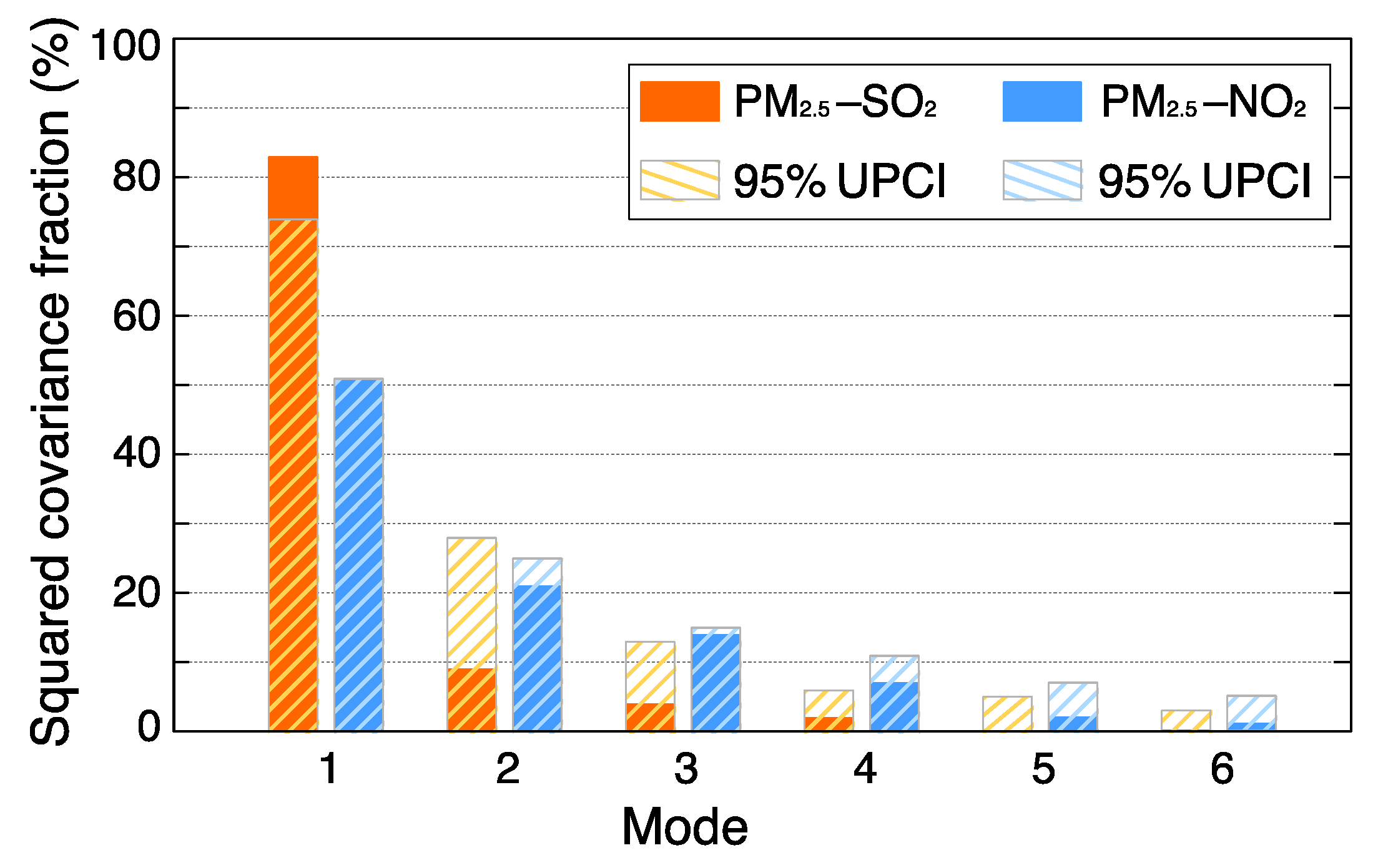
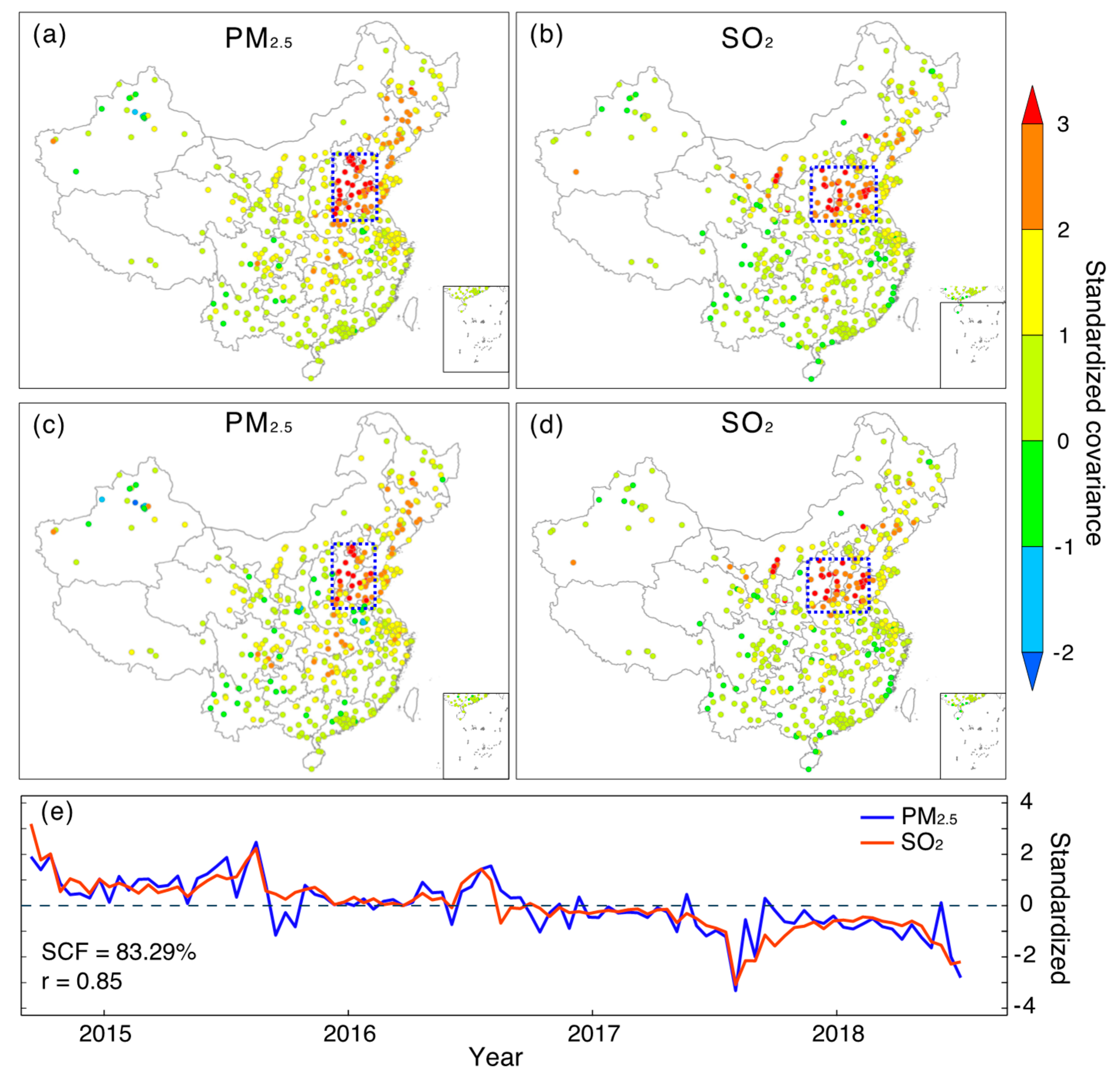
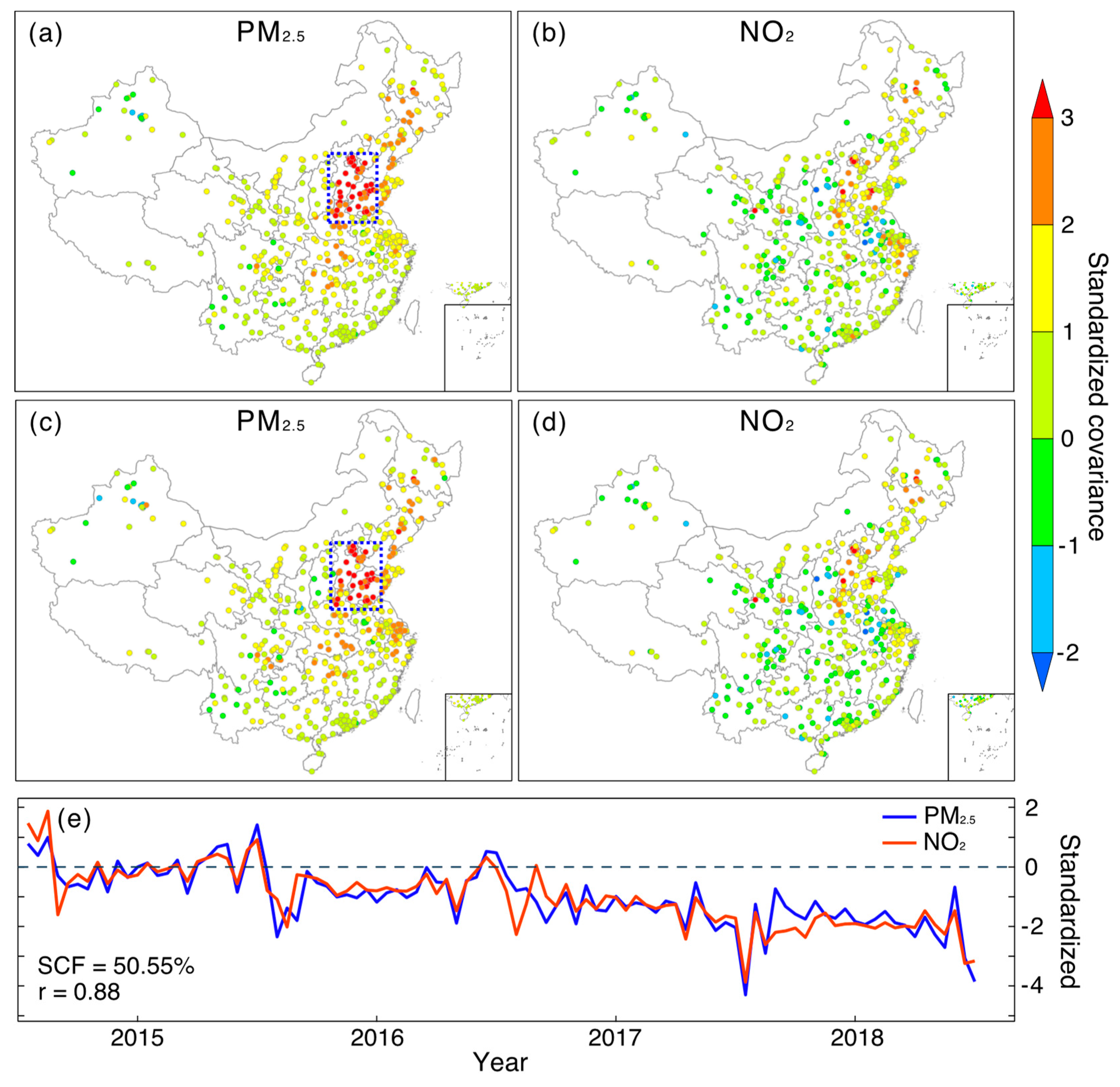
3.2. Spatiotemporal Coupled Patterns between PM_2.5 and SO₂ as well as NO₂

MCA was applied here to explore the spatiotemporal coupled patterns between PM_2.5 and SO₂ as well as NO₂. Prior to the analysis of coupled patterns, significance of each MCA mode was firstly assessed using Monte Carlo simulations. Figure 3 shows the estimated squared covariance fraction (SCF) of each MCA mode and the estimated upper limit at a 95% confidence interval (UPCI). In principle, only MCA modes with SCFs greater than the 95% UPCI are considered to be statistically significant. Apparently, only the first MCA mode of each pair passed the significance test. In other words, statistically significant linkages could be found from the first MCA modes between PM_2.5 and SO₂ and/or NO₂.

Given the significant test results, we only used the first MCA mode to explore possible coupled patterns between these three pollutants, to ensure the spatial patterns we extracted were statistically meaningful. It shows that the first MCA mode between PM_2.5 and SO₂ explained more than 80% of the observed covariance, indicating a tight spatiotemporal co-varying pattern between PM_2.5 and SO₂ across China. This effect could be also linked to the observed coincident declining trends for both pollutants. In contrast, the first MCA mode between PM_2.5 and NO₂ only explained about 50% of the covariance, indicating no uniform spatiotemporal variation pattern between these two factors. Given that PM_2.5 at most stations exhibited decreasing trends across China, the small SCF values associated with coupled modes between PM_2.5 and NO₂ thus suggest a significant heterogeneity of NO₂ variations nationwide. Such a deduction is also in line with the results previously shown in Figure 2, where heterogeneous NO₂ trends were observed across China.

Figure 4 and Figure 5 show the first MCA modes between PM_2.5 and SO₂ (Figure 4) as well as NO₂ (Figure 5), respectively. As indicated by both homogeneous and heterogeneous covariance maps (Figure 4a–d) as well as temporal variations (Figure 4e), there is an evident co-varying pattern between PM_2.5 and SO₂ in northern China. Specifically, the hot spot region for PM_2.5 is mainly located over regions in BTH and the west regions of Shandong province (the outlined region in Figure 4a). With respect to SO₂, regions exhibiting large covariance with PM_2.5 are also observed in northern China, but cover larger areas, as Shanxi province is also included. Such a highly clustered spatial pattern in both fields indicates that PM_2.5 and SO₂ in these regions share a similar variation pattern in temporal domain. Moreover, it indicates a far-reaching linkage between PM_2.5 and SO₂ in the spatial domain, as PM_2.5 in northern China may exhibit a similar variation pattern to that of SO₂, even in Shanxi province. Given PM_2.5 formations are highly associated with regional SO₂ emissions, we may suspect that the observed PM_2.5 variations in northern China might be modulated by not only local SO₂ emissions, but even emissions from neighboring regions like Shanxi province. Numerical simulations could be performed in the future to corroborate this inferred linkage, more specifically, to examine whether there is an eastward transfer of SO₂ emissions from Shanxi to northern China.

In contrast, no evident coupled field was found in the first MCA mode between PM_2.5 and NO₂ (Figure 5). Although a spatially localized PM_2.5 hot spot region was identified in northern China, no such effect was found in the NO₂ fields. Rather, stations with large covariance were observed to scatter randomly across China, indicating a lack of potent spatiotemporal coupled patterns between these two factors, regardless of the observed close correlation between their expansion coefficients (Figure 5e). In other words, the observed PM_2.5 variation in northern China had a weak linkage with local NO₂ emissions.

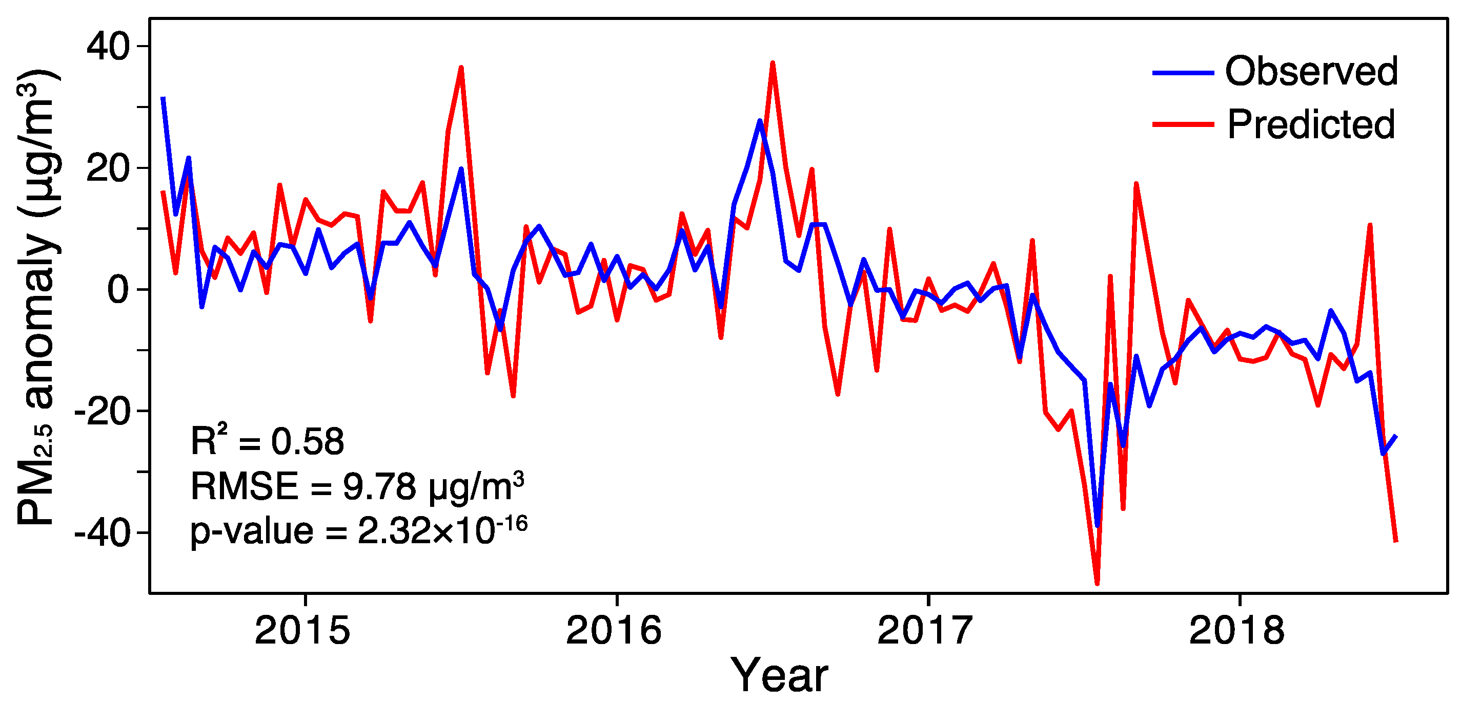
3.3. Relative Contributions of SO₂ and NO₂ to PM_2.5 Variations in Northern China

An MLR model was established to assess the relative contribution of SO₂ and NO₂ to PM_2.5 variations observed over northern China. First, PM_2.5 anomaly time series in northern China were extracted by averaging PM_2.5 anomaly time series at all stations located in BTH and nearby regions (i.e., hotspot regions identified from PM_2.5 homogeneity and heterogeneity covariance maps). The first two principal components (PC1 and PC2) of SO₂ and NO₂ (denoted as SO₂_PC1, SO₂_PC2, NO₂_PC1 and NO₂_PC2) were then extracted over the identified SO₂ hotspot region (outlined region in Figure 4b) and used as explanatory variables to proximate the observed PM_2.5 variations in northern China. All regressors were standardized by subtracting their mean values and then divided by their standard deviations to make them unitless and comparable. The MLR model can be expressed as:

$${\mathrm{PM}}_{2.5} ~ {\mathrm{SO}}_2\_\mathrm{PC}1+ {\mathrm{SO}}_2\_\mathrm{PC}2+{\mathrm{NO}}_2\_\mathrm{PC}1+{\mathrm{NO}}_2\_\mathrm{PC}2$$

(1)

Figure 6 simply compares the observed PM_2.5 variations in northern China and the predicted one, using the first two principal components of SO₂ and NO₂. It shows that about 58% (R² = 0.58) of the observed PM_2.5 variances can be explained by local SO₂ and NO₂ variations therein. Nonetheless, the predicted time series were prone to larger oscillations than the observed one.

Table 2. Estimated regression coefficients and LMG measures for each regressor. L-SPR (F-SPR) denotes the semi-partial coefficient of determination gains when the regressor was added as the least (first) regressor into the model. Numbers in brackets are percent variances explained by each principal component.

Regressor	Regression Coefficient	p-Value	LMG	L-SPR	F-SPR
SO2_PC1 (58.26%)	8.48	1.64 $\times {10}^{-5}$	0.31	0.10	0.53
SO2_PC2 (24.30%)	1.41	0.41	0.02	3.18 $\times {10}^{-3}$	0.03
NO2_PC1 (30.70%)	3.33	0.04	0.21	0.02	0.42
NO2_PC2 (24.07%)	0.20	0.92	0.03	4.72 $\times {10}^{-5}$	0.03

summarizes the regression coefficients and the estimated LMG measures for each regressor. It shows that only two regressors (SO₂_PC1 and NO₂_PC1) were statistically significant at the 95% confidence interval.

In terms of LMG measures, SO₂_PC1 had the largest LMG fraction, indicating the most significant role of SO₂ in contributing to the observed PM_2.5 variation. In contrast, NO₂_PC1 played a relative weak role. These effects were also evidenced by their semi-partial coefficient of determination (SPR), as the inclusion of SO₂_PC1 would result in salient improvement of R² regardless of the sequence. Since the largest value of estimated VIF between these four regressors was 1.93, which is far less than the threshold of 10, we may therefore claim that the collinearity between these four regressors can be neglected. In general, the modeling results clearly revealed the relative important role of SO₂ over NO₂ in contributing to the observed PM_2.5 variations in northern China from 2015 to 2018.

Nevertheless, this does not mean PM_2.5 variations in northern China have no inherent linkage with NO₂. Rather, there is no statistically significant linkage found between them in our cases. On the other hand, we should be aware of the fact that the temporal phase (i.e., warm versus cold or day versus night) of the relationship between PM_2.5 and NO₂ and SO₂ was not accounted for in the present study, though it plays critical roles in the formation of nitrates and sulfates [30,31,32]. The effect could be explored in the future by performing MCA analysis between PM_2.5 and day and/or night averaged NO₂ and SO₂ to better examine their possible linkage in space and time.

4. Conclusions

By taking advantage of in situ air quality records acquired from the China national air quality monitoring network, linear trends for PM_2.5, SO₂, and NO₂ were evaluated for the time period of 2015 to 2018. Prior to trend analysis, data values from neighboring stations were integrated on a semi-monthly basis to improve data completeness and to reduce dimensionality. The estimated linear trends indicate salient decreasing trends for PM_2.5 and SO₂, especially over northern China. Moreover, trends estimated from large values almost doubled those of the all-value averaged data, indicating the need to take data magnitudes into consideration in trend analysis in order to better assess the effectiveness of clean air actions. However, no evident decreasing trend was detected for NO₂ concentrations, even using their large data values.

The MCA results revealed an evident spatiotemporal coupled pattern between PM_2.5 and SO₂ in northern China from 2015 to 2018, but with different hot spot regions. Such an effect indicates a possible linkage that PM_2.5 variations in BTH might be attributed to SO₂ emissions, even in Shanxi province, to some degree. In contrast, no significant coupled pattern was found between PM_2.5 and NO₂. Further modeling practices revealed that about 58% of the observed PM_2.5 variations in northern China could be explained by local NO₂ and SO₂ variations collectively. Moreover, the observed PM_2.5 variations should be attributed largely to SO₂ variations in northern China, given the relatively larger importance found for SO₂ rather than NO₂. These results collectively suggest the need to implement more stringent emission control on NO₂ in China in the future. Given the constraint of temporal limitation of the in situ data record, a long-term study could be performed in the future by making use of satellite-derived PM_2.5 estimations and remotely sensed NO₂ and SO₂ columns, measured by the Ozone Monitoring Instrument (OMI), to better explore their associations in space and time.

References

1. Bai, K.; Ma, M.; Chang, N.-B.; Gao, W. Spatiotemporal trend analysis for fine particulate matter concentrations in China using high-resolution satellite-derived and ground-measured PM2.5 data. J. Environ. Manag. 2019, 233, 530–542. [Google Scholar] [CrossRef] [PubMed]
2. Cai, S.; Wang, Y.; Zhao, B.; Wang, S.; Chang, X.; Hao, J. The impact of the “Air Pollution Prevention and Control Action Plan” on PM2.5 concentrations in Jing–Jin–Ji region during 2012–2020. Sci. Total Environ. 2017, 580, 197–209. [Google Scholar] [CrossRef] [PubMed]
3. Zheng, Y.; Xue, T.; Zhang, Q.; Geng, G.; Tong, D.; Li, X.; He, K. Air quality improvements and health benefits from China’s clean air action since 2013. Environ. Res. Lett. 2017, 12. [Google Scholar] [CrossRef]
4. Xie, Y.; Zhao, B.; Zhang, L.; Luo, R. Spatiotemporal variations of PM2.5 and PM10 concentrations between 31 Chinese cities and their relationships with SO2, NO2, CO and O3. Particuology 2015, 20, 141–149. [Google Scholar] [CrossRef]
5. Huang, X.H.H.; Bian, Q.; Ng, W.M.; Louie, P.K.K.; Yu, J.Z. Characterization of PM2.5 Major Components and Source Investigation in Suburban Hong Kong: A One Year Monitoring Study. Aerosol Air Qual. Res. 2014, 14, 237–250. [Google Scholar] [CrossRef]
6. Xue, J.; Yuan, Z.; Griffith, S.M.; Yu, X.; Lau, A.K.H.; Yu, J.Z. Sulfate Formation Enhanced by a Cocktail of High NOx, SO2, Particulate Matter, and Droplet pH during Haze-Fog Events in Megacities in China: An Observation-Based Modeling Investigation. Environ. Sci. Technol. 2016, 50, 7325–7334. [Google Scholar] [CrossRef] [PubMed]
7. Ye, W.-F.; Ma, Z.-Y.; Ha, X.-Z. Spatial-temporal patterns of PM2.5 concentrations for 338 Chinese cities. Sci. Total Environ. 2018, 631–632, 524–533. [Google Scholar] [CrossRef]
8. Ma, Z.; Hu, X.; Sayer, A.M.; Levy, R.; Zhang, Q.; Xue, Y.; Tong, S.; Bi, J.; Huang, L.; Liu, Y. Satellite-based spatiotemporal trends in PM2.5 concentrations: China, 2004–2013. Environ. Health Perspect. 2016, 124, 184–192. [Google Scholar] [CrossRef]
9. Mi, K.; Zhuang, R.; Zhang, Z.; Gao, J.; Pei, Q. Spatiotemporal characteristics of PM2.5 and its associated gas pollutants, a case in China. Sustain. Cities Soc. 2019, 45, 287–295. [Google Scholar] [CrossRef]
10. Si, Y.; Yu, C.; Zhang, L.; Zhu, W.; Cai, K.; Cheng, L.; Chen, L.; Li, S. Assessment of satellite-estimated near-surface sulfate and nitrate concentrations and their precursor emissions over China from 2006 to 2014. Sci. Total Environ. 2019, 669, 362–376. [Google Scholar] [CrossRef]
11. Li, K.; Jacob, D.J.; Liao, H.; Shen, L.; Zhang, Q.; Bates, K.H. Anthropogenic drivers of 2013–2017 trends in summer surface ozone in China. Proc. Natl. Acad. Sci. 2019, 116, 422–427. [Google Scholar] [CrossRef]
12. Yang, D.; Wang, X.; Xu, J.; Xu, C.; Lu, D.; Ye, C.; Wang, Z.; Bai, L. Quantifying the influence of natural and socioeconomic factors and their interactive impact on PM2.5 pollution in China. Environ. Pollut. 2018, 241, 475–483. [Google Scholar] [CrossRef] [PubMed]
13. Yang, Q.; Yuan, Q.; Yue, L.; Li, T.; Shen, H.; Zhang, L. The relationships between PM2.5 and aerosol optical depth (AOD) in mainland China: About and behind the spatio-temporal variations. Environ. Pollut. 2019, 248, 526–535. [Google Scholar] [CrossRef]
14. Zhong, J.; Zhang, X.; Wang, Y. Relatively weak meteorological feedback effect on PM2.5 mass change in Winter 2017/18 in the Beijing area: Observational evidence and machine-learning estimations. Sci. Total Environ. 2019, 664, 140–147. [Google Scholar] [CrossRef] [PubMed]
15. Behera, S.N.; Sharma, M. Degradation of SO2, NO2 and NH3 leading to formation of secondary inorganic aerosols: An environmental chamber study. Atmos. Environ. 2011, 45, 4015–4024. [Google Scholar] [CrossRef]
16. Hsu, Y.-M.; Clair, T.A. Measurement of fine particulate matter water-soluble inorganic species and precursor gases in the Alberta Oil Sands Region using an improved semicontinuous monitor. J. Air Waste Manag. Assoc. 2015, 65, 423–435. [Google Scholar] [CrossRef] [PubMed]
17. Bretherton, C.S.; Smith, C.; Wallace, J.M. An Intercomparison of Methods for Finding Coupled Patterns in Climate Data. J. Clim. 1992, 5, 541–560. [Google Scholar] [CrossRef] [Green Version]
18. Wallace, J.M.; Smith, C.; Bretherton, C.S. Singular Value Decomposition of Wintertime Sea Surface Temperature and 500-mb Height Anomalies. J. Clim. 1992, 5, 561–576. [Google Scholar] [CrossRef]
19. Bai, K.; Chang, N.-B.; Gao, W. Quantification of relative contribution of Antarctic ozone depletion to increased austral extratropical precipitation during 1979–2013. J. Geophys. Res. Atmos. 2016, 121, 1459–1474. [Google Scholar] [CrossRef]
20. Ding, Q.; Steig, E.J.; Battisti, D.S.; Küttel, M. Winter warming in West Antarctica caused by central tropical Pacific warming. Nat. Geosci. 2011, 4, 398–403. [Google Scholar] [CrossRef] [Green Version]
21. Casey, K.S. Sea surface temperature and sea surface height variability in the North Pacific Ocean from 1993 to 1999. J. Geophys. Res. 2002, 107, 3099. [Google Scholar] [CrossRef]
22. Wu, Q. Observed impact of subtropical-midlatitude South Atlantic SST anomalies on the atmospheric circulation. Geophys. Res. Lett. 2008, 35. [Google Scholar] [CrossRef]
23. Hu, Q. On the Uniqueness of the Singular Value Decomposition in Meteorological Applications. J. Clim. 1997, 10, 1762–1766. [Google Scholar] [CrossRef]
24. Coelho, C.A.S.; Uvo, C.B.; Ambrizzi, T. Exploring the impacts of the tropical Pacific SST on the precipitation patterns over South America during ENSO periods. Theor. Appl. Climatol. 2002, 71, 185–197. [Google Scholar] [CrossRef]
25. Qiao, S.; Gong, Z.; Feng, G.; Qian, Z. Relationship between cold winters over Northern Asia and the subsequent hot summers over mid-lower reaches of the Yangtze River valley under global warming. Atmos. Sci. Lett. 2015, 16, 479–484. [Google Scholar] [CrossRef]
26. Renwick, J.A.; Wallace, J.M. Predictable Anomaly Patterns and the Forecast Skill of Northern Hemisphere Wintertime 500-mb Height Fields. Mon. Weather Rev. 1995, 123, 2114–2131. [Google Scholar] [CrossRef] [Green Version]
27. Frankignoul, C.; Chouaib, N.; Liu, Z. Estimating the Observed Atmospheric Response to SST Anomalies: Maximum Covariance Analysis, Generalized Equilibrium Feedback Assessment, and Maximum Response Estimation. J. Clim. 2011, 24, 2523–2539. [Google Scholar] [CrossRef] [Green Version]
28. Brien, R.M.O. A Caution Regarding Rules of Thumb for Variance Inflation Factors. Qual. Quant. 2007, 41, 637–690. [Google Scholar] [CrossRef]
29. Grömping, U. Relative Importance for Linear Regression in R: The Package relaimpo. J. Stat. Softw. 2006, 17, 1–27. [Google Scholar] [CrossRef]
30. Guo, H.; Liu, J.; Froyd, K.D.; Roberts, J.M.; Veres, P.R.; Hayes, P.L.; Jimenez, J.L.; Nenes, A.; Weber, R.J. Fine Particle pH and Gas-Particle Phase Partitioning of Inorganic Species in Pasadena, California, during the 2010 CalNex Campaign. Atmos. Chem. Phys. 2017, 17, 5703–5719. [Google Scholar] [CrossRef]
31. Vasilakos, P.; Russell, A.; Weber, R.; Nenes, A. Understanding Nitrate Formation in A World with Less Sulfate. Atmos. Chem. Phys. 2018, 18, 12765–12775. [Google Scholar] [CrossRef]
32. Dawson, J.P.; Adams, P.J.; Pandis, S.N. Sensitivity of PM2.5 to Climate in the Eastern US: A Modeling Case Study. Atmos. Chem. Phys. 2007, 7, 4295–4309. [Google Scholar] [CrossRef]
Figure 1. The seven major Chinese geographic divisions (a) and an illustrative example of spatial hierarchy clustering (b). Gray dots represent the original monitoring stations and blue crosses denote the aggregated stations after spatial clustering.
Ijerph 16 02352 g001
Figure 2. Site-specific linear trends for PM2.5 (fine particulate matter), SO2 and NO2 at 499 clustered stations across China from January 2015 to December 2018. (ac) Trends derived from all data value averaged PM2.5, SO2 and NO2 concentrations; (df) trends derived from large values (averaged for values greater than the fourth quartile). Note that the radius of circles varies with the magnitudes of trend values, and the hollow circles indicate trends that failed to pass the significant test at the 95% confidence level.
Ijerph 16 02352 g002
Figure 3. Squared covariance fraction for the first six maximum covariance analysis (MCA) modes between PM2.5 and SO2 as well as NO2, where 95% UPCI (upper limit of confidence interval) denotes the estimated squared covariance fraction at the 95% quantile of all values derived from the Monte Carlo simulations.
Ijerph 16 02352 g003
Figure 4. The first MCA mode between PM2.5 and SO2 coupled in the spatial and temporal domains. (ab) Homogeneous covariance maps (covariance between expansion coefficient and time series of the same original field); (cd) heterogeneous covariance maps (covariance between expansion coefficient and time series of another field); (e) standardized expansion coefficient (divided by their standard deviations) of the first MCA mode. Note that the annual cycle has been removed from each field prior to MCA analysis.
Ijerph 16 02352 g004
Figure 5. Same as Figure 4, but for coupled fields between PM2.5 and NO2. (ab) Homogeneous covariance maps (covariance between expansion coefficient and time series of the same original field); (cd) heterogeneous covariance maps (covariance between expansion coefficient and time series of another field); (e) standardized expansion coefficient (divided by their standard deviations) of the first MCA mode.
Ijerph 16 02352 g005
Figure 6. Comparison of the observed PM2.5 variations in northern China and the predicted one. Note that the annual cycles have been removed from each variable prior to modeling analysis.
Ijerph 16 02352 g006