Joint Risk of Rainfall and Storm Surges during Typhoons in a Coastal City of Haidian Island, China


Abstract
1. Introduction
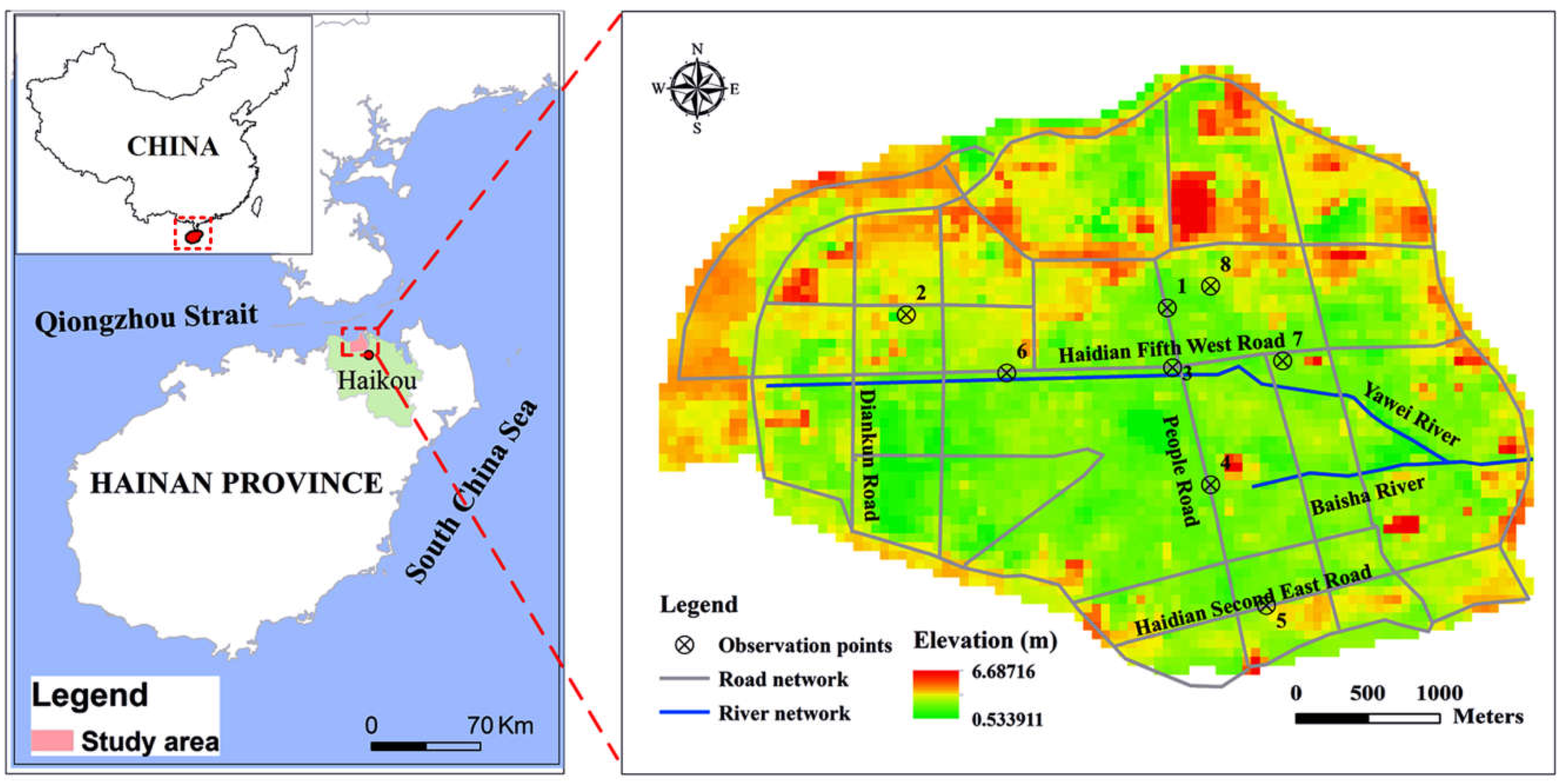
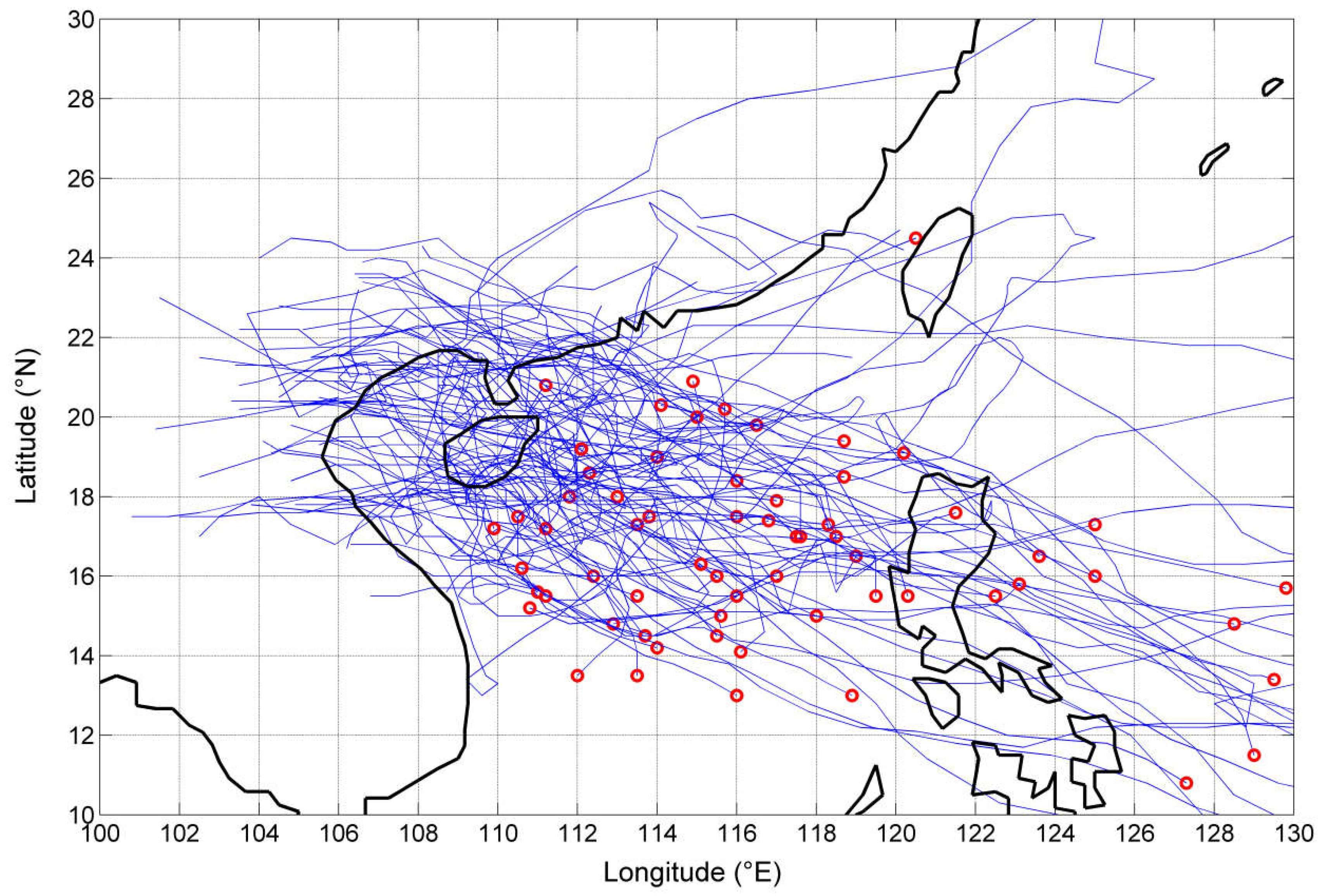
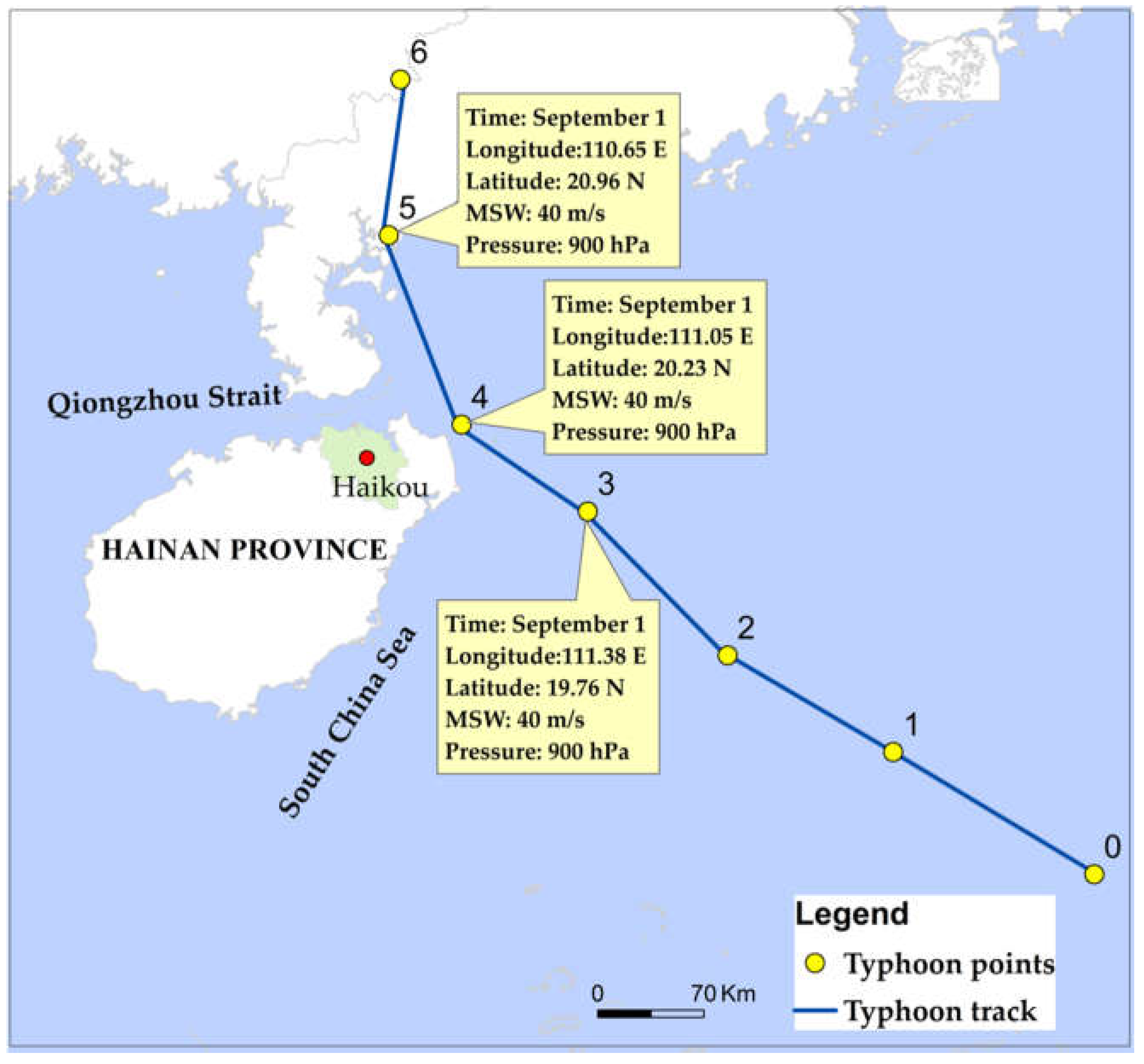
2. Study Area and Data
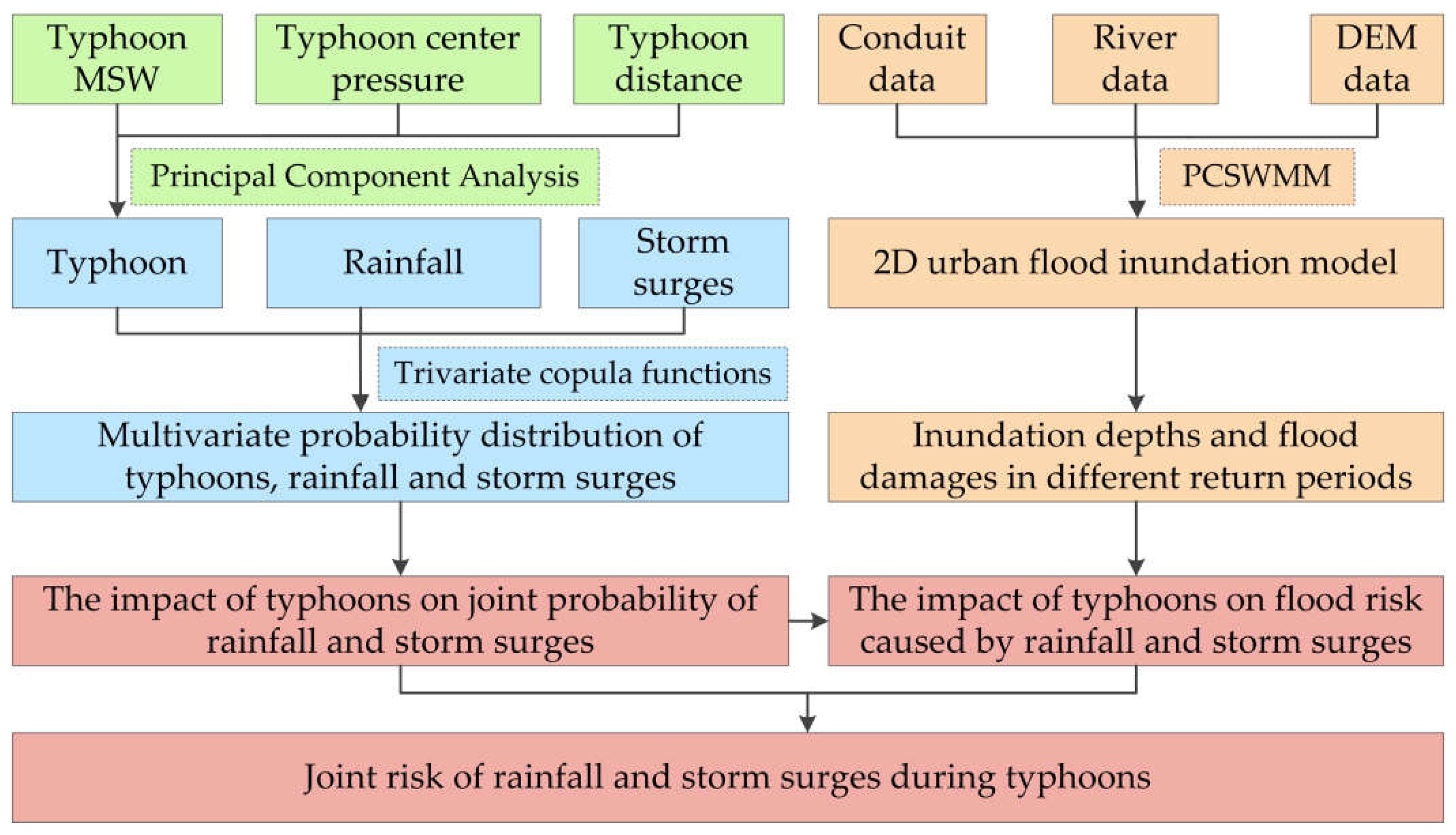
3. Methods
3.1. Principal Component Analysis
3.2. Copula Function
3.3. Expected Annual Damage Evaluation
4. Results and Discussion
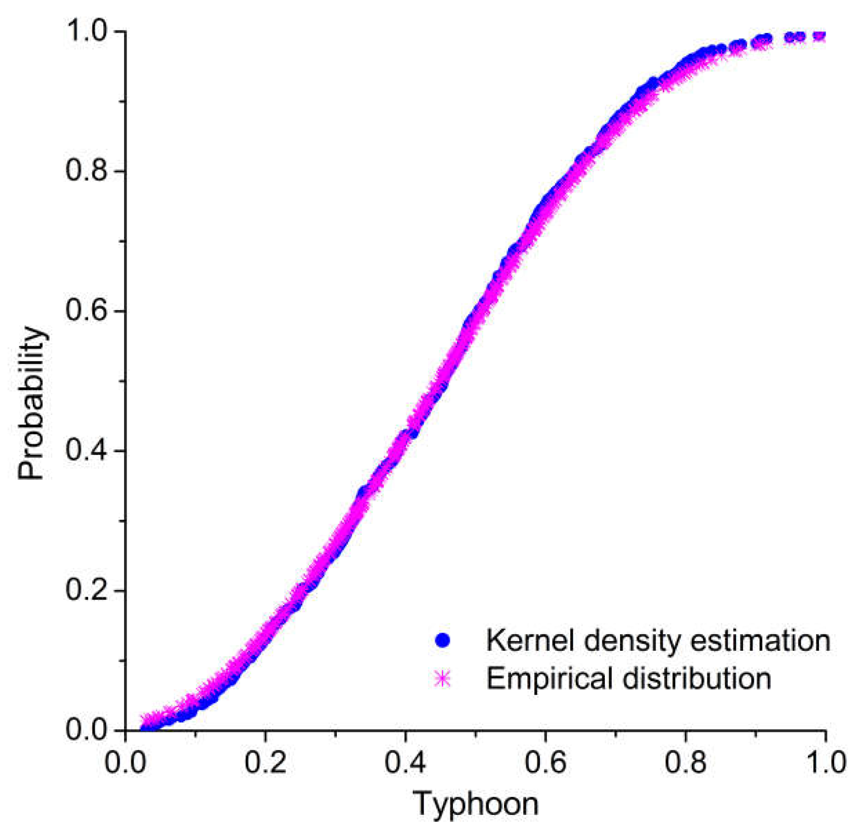
4.1. Quantification of Typhoons
4.2. Multivariate Joint Probability Distribution of Typhoons, Rainfall, and Storm Surges
4.2.1. Correlation among Typhoons, Rainfall, and Storm Surges
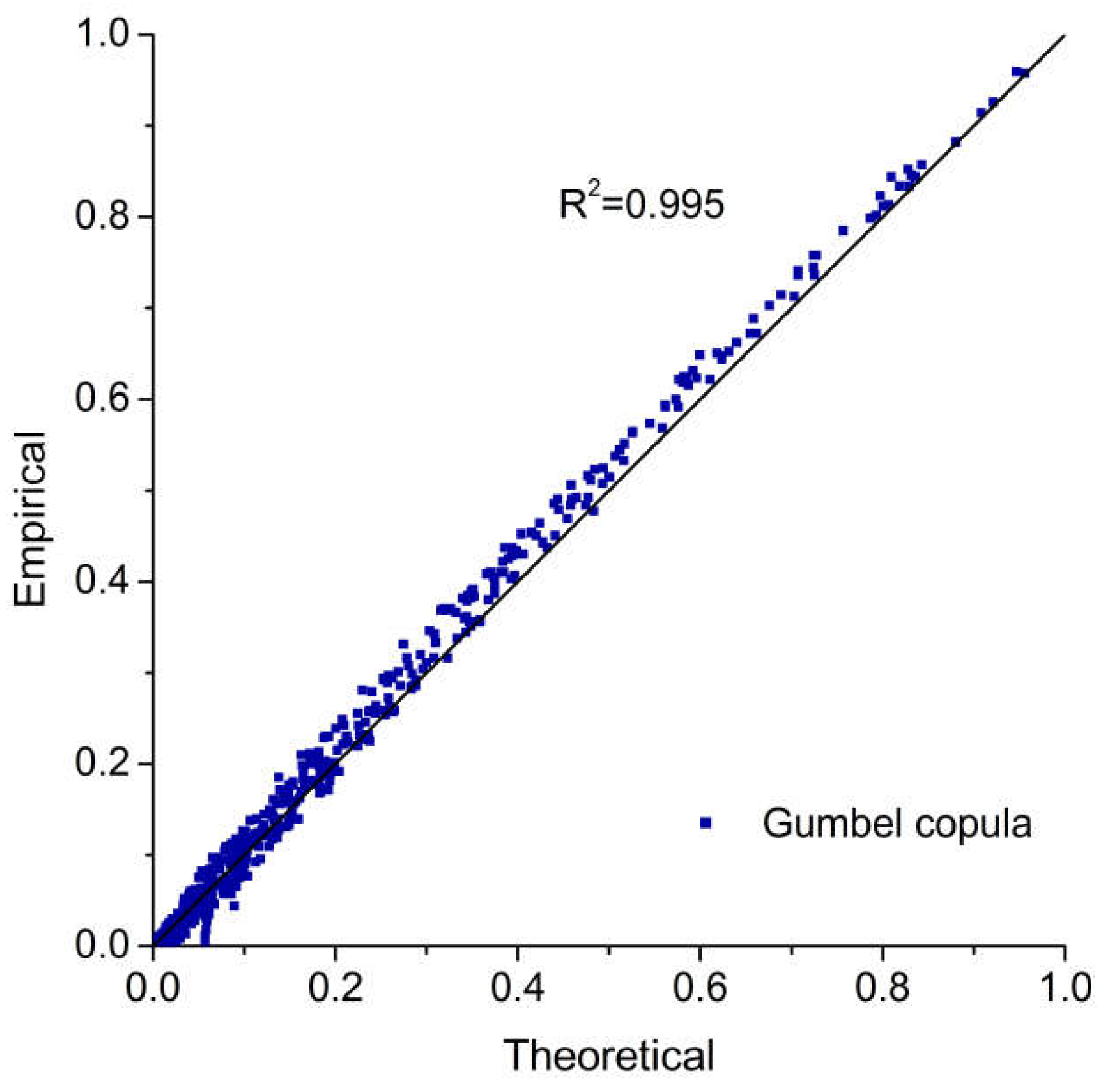
4.2.2. Trivariate Joint Probability Distribution of Typhoon–Rainfall–Storm Surge
4.2.3. Joint Probability of Typhoon–Rainfall–Storm Surge Analysis
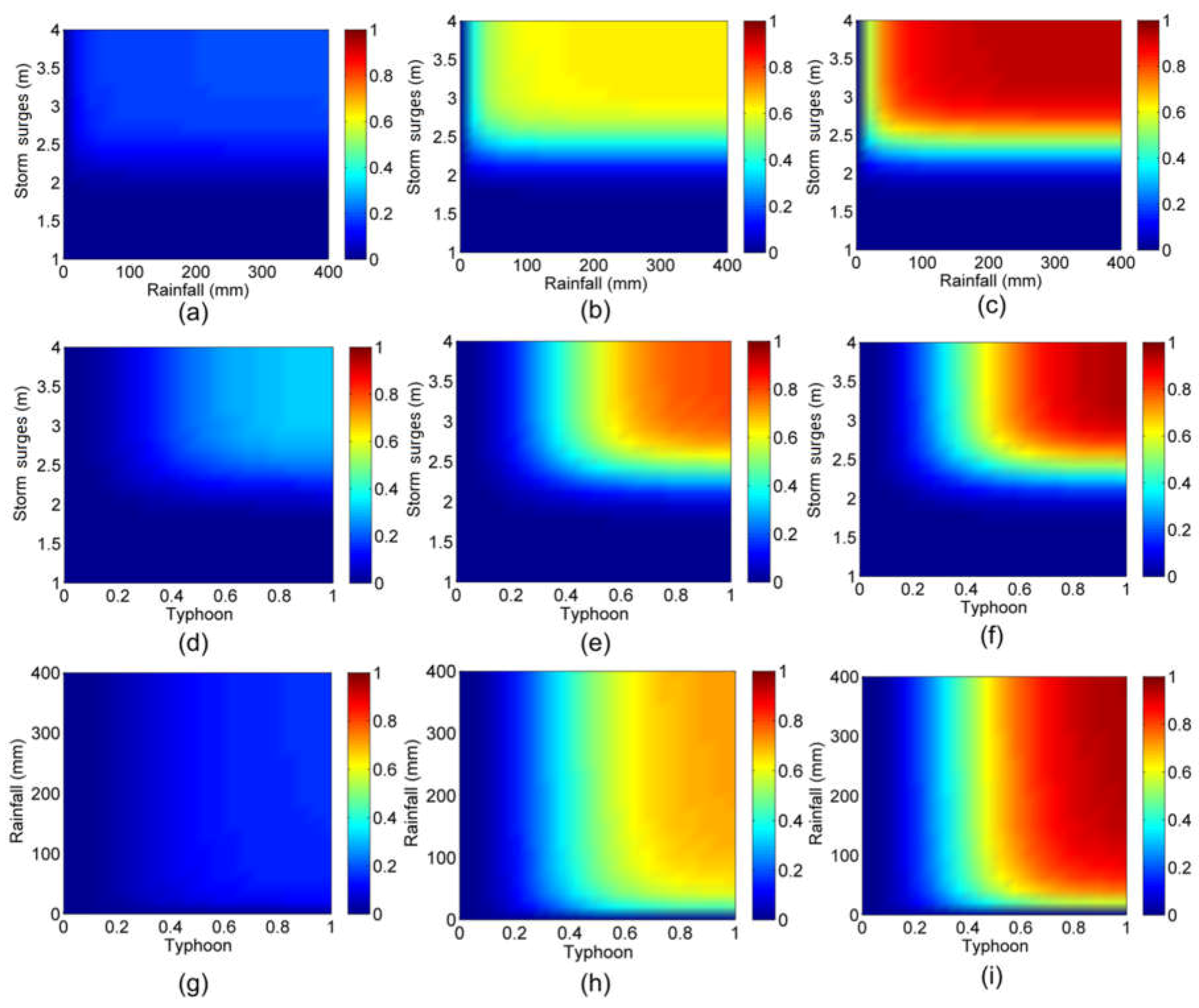
4.3. Joint Risk of Rainfall and Storm Surges during Typhoons on Haidian Island
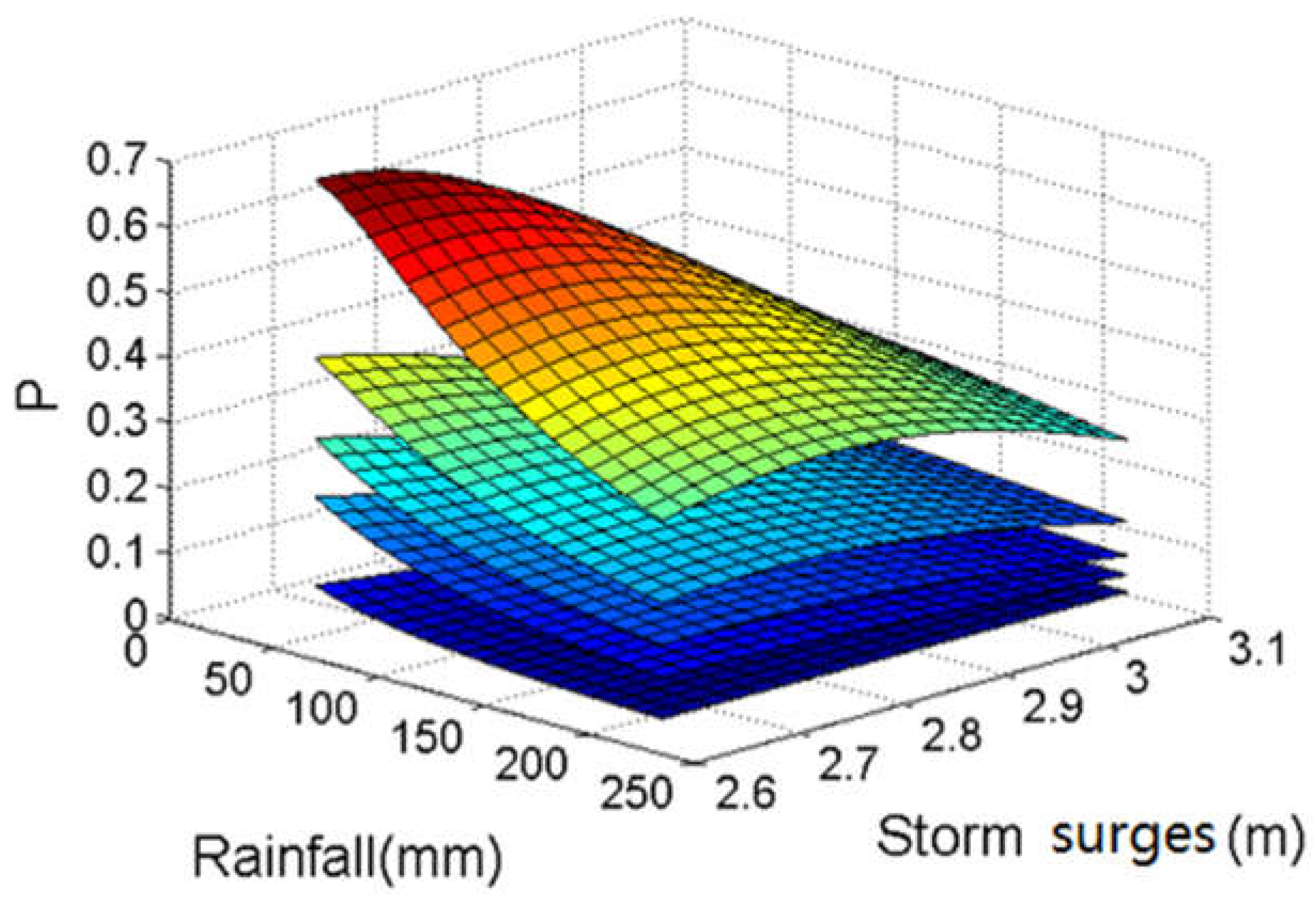
4.3.1. Impact of Typhoons on Joint Probability of Rainfall and Storm Surges
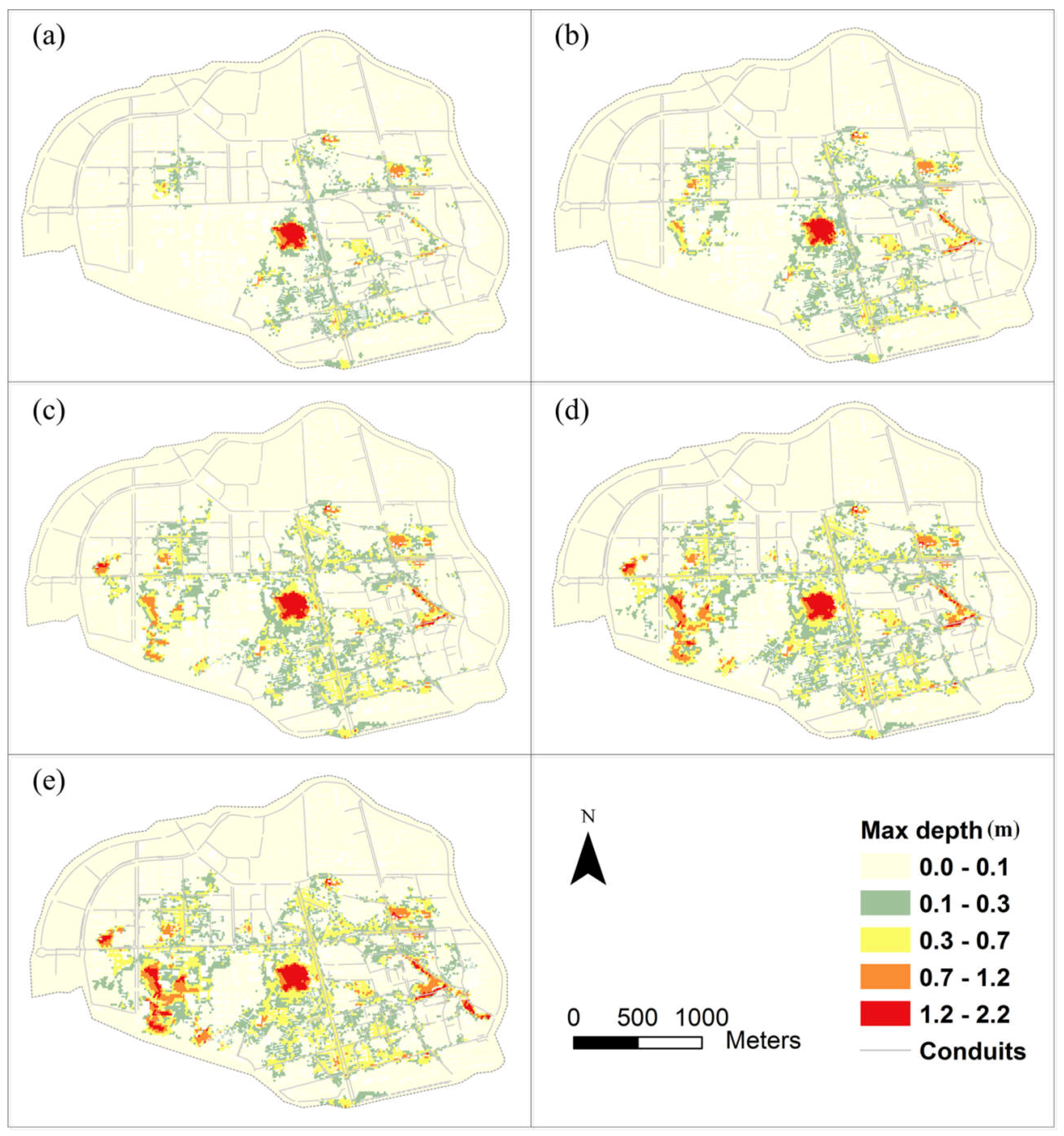
4.3.2. Impact of Typhoons on Flood Risk Caused by Rainfall and Storm Surges
5. Conclusions
Author Contributions
Funding
Acknowledgments
Conflicts of Interest
Appendix A. Introduction of Copula Functions

| Copulas | C(u,v) |
|---|---|
| Gumbel | |
| Clayton | |
| Frank | |
| Gaussian | |
| Student’s t |
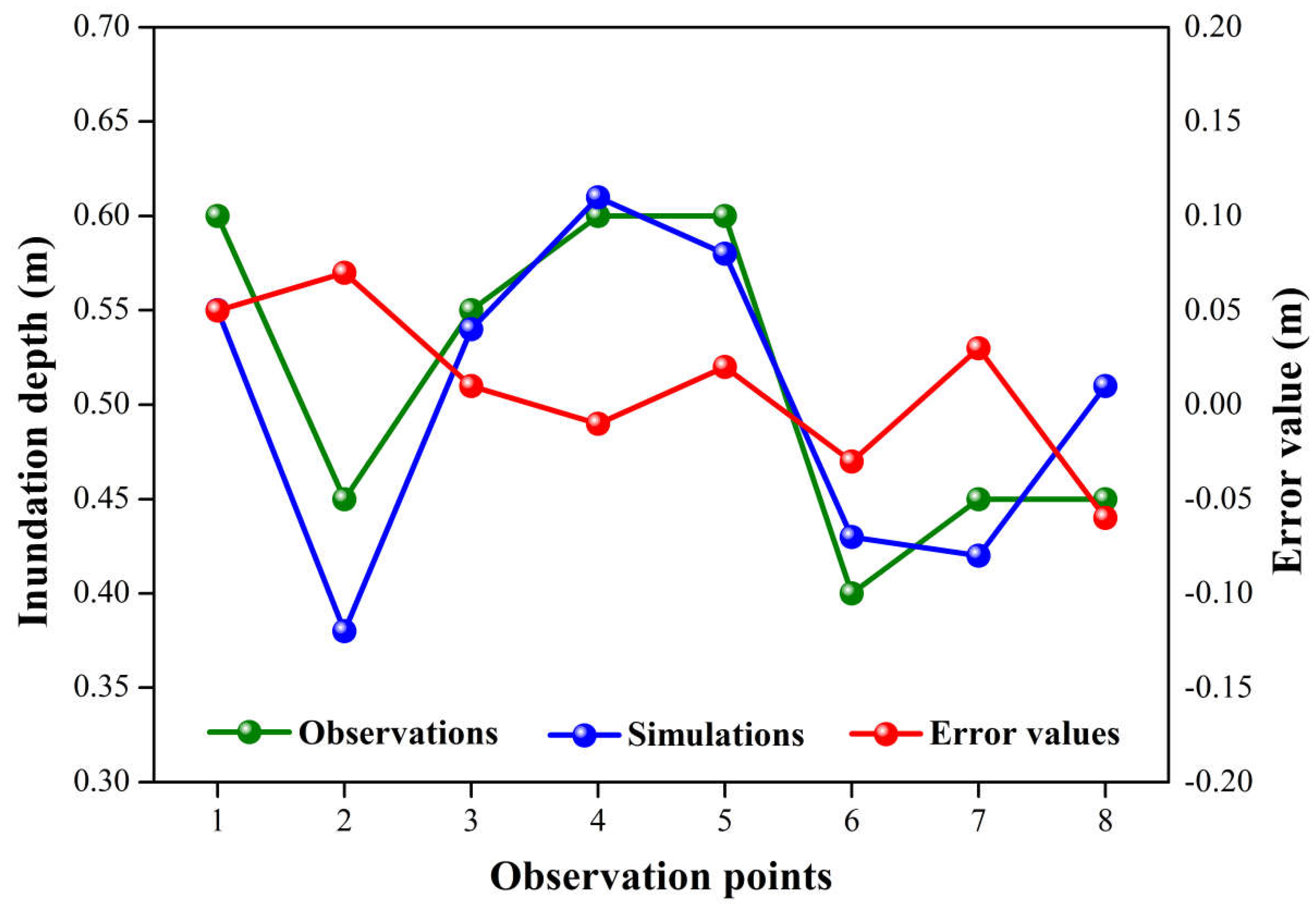
Appendix B. Urban Flood Inundation Model on Haidian Island

References
- Zhang, W.; Wang, W.; Lin, J.; Zhang, Y.; Shang, X.; Wang, X.; Huang, M.; Liu, S.; Ma, W. Perception, Knowledge and Behaviors Related to Typhoon: A Cross Sectional Study among Rural Residents in Zhejiang, China. Int. J. Environ. Res. Public Health 2017, 14, 492. [Google Scholar] [CrossRef] [PubMed]
- Zhong, H.; Van Overloop, P.J.; van Gelder, P.H.A.J.M. A joint probability approach using a 1-D hydrodynamic model for estimating high water level frequencies in the Lower Rhine Delta. Nat. Hazard Earth Syst. 2013, 13, 1841–1852. [Google Scholar] [CrossRef]
- Zheng, F.; Westra, S.; Sisson, S. Quantifying the dependence between extreme rainfall and storm surge in the coastal zone. J. Hydrol. 2013, 505, 172–187. [Google Scholar] [CrossRef]
- Zheng, F.; Seth, W.; Michael, L.; Sisson, S. Modeling dependence between extreme rainfall and storm surge to estimate coastal flooding risk. Water Resour. Res. 2014, 50, 2050–2071. [Google Scholar] [CrossRef]
- Lian, J.; Xu, K.; Ma, C. Joint impact of rainfall and tidal level on flood risk in a coastal city with a complex river network: A case study of Fuzhou City, China. Hydrol. Earth Syst. Sci. 2013, 17, 679–689. [Google Scholar] [CrossRef]
- Archetti, R.; Bolognesi, A.; Casadio, A.; Maglionico, M. Development of flood probability charts for urban drainage network in coastal areas through a simplified joint assessment approach. Hydrol. Earth Syst. Sci. 2011, 15, 3115–3122. [Google Scholar] [CrossRef]
- Xu, K.; Ma, C.; Lian, J.; Bin, L. Joint probability analysis of extreme precipitation and storm tide in a coastal city under changing environment. PLoS ONE 2014, 9, e109341. [Google Scholar] [CrossRef] [PubMed]
- Hurk, B.V.D.; Meijgaard, E.V.; Valk, P.D.; van Heeringen, K.-J.; Gooijer, J. Analysis of a compounding surge and precipitation event in the Netherlands. Environ. Res. Lett. 2015, 10, 035001. [Google Scholar] [CrossRef]
- Wu, Z.; Zhao, L.; Ge, Y. Statistical analysis of wind velocity and rainfall intensity joint probability distribution of Shanghai area in typhoon condition. Acta Aerodyn. Sin. 2010, 28, 393–399. [Google Scholar]
- Dong, S.; Jiao, C.; Tao, S. Joint return probability analysis of wind speed and rainfall intensity in typhoon-affected sea area. Nat. Hazards 2017, 86, 1193–1205. [Google Scholar] [CrossRef]
- Konrad, C.E. The most extreme precipitation events over the eastern United States from 1950 to 1996: Considerations of scale. J. Hydrometeorol. 2001, 2, 309–325. [Google Scholar] [CrossRef]
- Matyas, C.J. Associations between the size of hurricane rain fields at landfall and their surrounding environments. Meteorol. Atmos. Phys. 2010, 106, 135–148. [Google Scholar] [CrossRef]
- Zhu, L.; Quiring, S.M.; Emanuel, K.A. Estimating tropical cyclone precipitation risk in Texas. Geophys. Res. Lett. 2013, 40, 6225–6230. [Google Scholar] [CrossRef]
- Lonfat, M.; Marks, F.D.; Chen, S. Precipitation distribution in tropical cyclones using the Tropical Rainfall Measuring Mission (TRMM) Microwave Imager: A global perspective. Mon. Weather. Rev. 2004, 132, 1645–1660. [Google Scholar] [CrossRef]
- Wang, Z.; Liu, G.; Gong, Z.; Zhang, C. Exceeding cumulative probability analysis of seawall considering the joint probability distribution of tide level and wind speed. Adv. Sci. Technol. Water Resour. 2014, 34, 18–22. [Google Scholar]
- Zhang, L.; Singh, V. Bivariate flood frequency analysis using the copula method. J. Hydrol. Eng. 2006, 11, 150–164. [Google Scholar] [CrossRef]
- Chebana, F.; Ouarda, T. Index flood-based multivariate regional frequency analysis. Water Resour. Res. 2009, 45, W10435. [Google Scholar] [CrossRef]
- Li, F.; Zheng, Q. Probabilistic modelling of flood events using the entropy copula. Adv. Water Resour. 2016, 97, 233–240. [Google Scholar] [CrossRef]
- Eagleson, P.S. Dynamics of flood frequency. Water Resour. Res. 1972, 8, 878–898. [Google Scholar] [CrossRef]
- Goel, N.K.; Kurothe, R.S.; Mathur, B.S.; Vogel, R.M. A derived flood frequency distribution for correlated rainfall intensity and duration. J. Hydrol. 2000, 228, 56–67. [Google Scholar] [CrossRef]
- Zhang, L.; Singh, V. Bivariate rainfall frequency distributions using Archimedean copulas. J. Hydrol. 2007, 332, 93–109. [Google Scholar] [CrossRef]
- Kao, S.; Govindaraju, R. Probabilistic structure of storm surface runoff considering the dependence between average intensity and storm duration of rainfall events. Water Resour. Res. 2007, 43, W06410. [Google Scholar] [CrossRef]
- Vandenberghe, S.; Verhoest, N.; De Baets, B. Fitting bivariate copulas to the dependence structure between storm characteristics: A detailed analysis based on 105 year 10 min rainfall. Water Resour. Res. 2010, 46, 489–496. [Google Scholar] [CrossRef]
- Zhang, Q.; Singh, V.; Li, J.; Jiang, F.; Bai, Y. Spatio-temporal variations of precipitation extremes in Xinjiang, China. J. Hydrol. 2012, 434–435, 7–18. [Google Scholar] [CrossRef]
- Wang, Y.; Li, C.; Liu, J.; Yu, F.; Qiu, Q.; Tian, J. Multivariate analysis of joint probability of different rainfall frequencies based on copulas. Water 2017, 9, 198. [Google Scholar] [CrossRef]
- Lee, T.; Modarres, R.; Ouarda, T. Data-based analysis of bivariate copula tail dependence for drought duration and severity. Hydrol. Process. 2012, 27, 1454–1463. [Google Scholar] [CrossRef]
- Saghafian, B.; Mehdikhani, H. Drought characterization using a new copula-based trivariate approach. Nat. Hazards 2013, 72, 1391–1407. [Google Scholar] [CrossRef]
- Ma, M.; Song, S.; Ren, L.; Jiang, S.; Song, J. Multivariate drought characteristics using trivariate gaussian and student t copulas. Hydrol. Process. 2013, 27, 1175–1190. [Google Scholar] [CrossRef]
- Xu, K.; Yang, D.; Xu, X.; Lei, H. Copula based drought frequency analysis considering the spatio-temporal variability in southwest China. J. Hydrol. 2015, 527, 630–640. [Google Scholar] [CrossRef]
- Zhao, P.; Lü, H.; Fu, G.; Zhu, Y.; Su, J.; Wang, J. Uncertainty of hydrological drought characteristics with copula functions and probability distributions: A case study of Weihe river, China. Water 2017, 9, 334. [Google Scholar] [CrossRef]
- Tariq, M.A.U.R. Risk-based flood zoning employing expected annual damages: The Chenab river case study. Stoch. Environ. Res. Risk Assess. 2013, 27, 1957–1966. [Google Scholar] [CrossRef]
- Lian, J.J.; Xu, H.S.; Xu, K.; Ma, C. Optimal management of the flooding risk caused by the joint occurrence of extreme rainfall and high tide level in a coastal city. Nat. Hazards 2017, 89, 183–200. [Google Scholar] [CrossRef]
- Tillinghast, E.D.; Hunt, W.F.; Jennings, G.D.; D’Arconte, P. Increasing stream geomorphic stability using storm water control measures in a densely urbanized watershed. J. Hydrol. Eng. 2012, 17, 1381–1388. [Google Scholar] [CrossRef]
- Ahiablame, L.; Shakya, R. Modeling flood reduction effects of low impact development at a watershed scale. J. Environ. Manag. 2016, 171, 81. [Google Scholar] [CrossRef] [PubMed]
- Akhter, M.S.; Hewa, G.A. The use of PCSWMM for assessing the impacts of land use changes on hydrological responses and performance of WSUD in managing the impacts at Myponga catchment, South Australia. Water 2016, 8, 511. [Google Scholar] [CrossRef]
- Paule-Mercado, M.A.; Lee, B.Y.; Memon, S.A.; Umer, S.R.; Salim, I.; Lee, C.H. Influence of land development on stormwater runoff from a mixed land use and land cover catchment. Sci. Total Environ. 2017, 599–600, 2142–2155. [Google Scholar] [CrossRef] [PubMed]
- Rossman, L.A. Storm Water Management Model User’s Manual; U.S. Environmental Protection Agency: Cincinnaty, OH, USA, 2015.
- Knapp, K.R.; Kruk, M.C.; Levinson, D.H.; Diamond, H.J.; Neumann, C.J. The International Best Track Archive for Climate Stewardship (IBTrACS): Unifying tropical cyclone data. Bull. Amer. Meteorol. Soc. 2010, 91, 363–376. [Google Scholar] [CrossRef]
- Ying, M.; Zhang, W.; Yu, H.; Lu, X.; Feng, J.; Fan, Y.; Zhu, Y.L.; Zhu, D. An overview of the China Meteorological Administration tropical cyclone database. J. Atmos. Ocean. Technol. 2014, 31, 287–301. [Google Scholar] [CrossRef]
- Jiang, H.Y.; Zipser, E.J. Contribution of tropical cyclones to the global precipitation from eight seasons of TRMM data: Regional, seasonal, and interannual variations. J. Clim. 2010, 23, 264–279. [Google Scholar] [CrossRef]
- Nogueira, R.C.; Keim, B.D. Contributions of Atlantic tropical cyclones to monthly and seasonal rainfall in the eastern United States 1960–2007. Theor. Appl. Climatol. 2011, 103, 213–227. [Google Scholar] [CrossRef]
- Witte, K.; Schobesberger, H.; Peham, C. Motion pattern analysis of gait in horseback riding by means of principal component analysis. Hum. Mov. Sci. 2009, 28, 394–405. [Google Scholar] [CrossRef] [PubMed]
- Jolliffe, I.T.; Cadima, J. Principal component analysis: A review and recent developments. Philos. Trans. A Math. Phys. Eng. Sci. 2016, 374, 20150202. [Google Scholar] [CrossRef] [PubMed]
- Ye, X.; Liu, G.; Liu, H.; Li, S. Study on model of aroma quality evaluation for flue-cured tobacco based on principal component analysis. J. Food Agric. Environ. 2011, 9, 501–504. [Google Scholar]
- Fernandez, P.; Mourato, S.; Moreira, M.; Pereira, L. A new approach for computing a flood vulnerability index using cluster analysis. Phys. Chem. Earth Parts A/B/C 2016, 94, 47–55. [Google Scholar] [CrossRef]
- Sklar, M. Fonctions de Répartition à n Dimensions et Leurs Marges; Université Paris 8: Saint-Denis, France, 1959. [Google Scholar]
- Madadgar, S.; Moradkhani, H. Drought analysis under climate change using copula. J. Hydrol. Eng. 2013, 18, 746–759. [Google Scholar] [CrossRef]
- Ganguli, P.; Reddy, M.J. Evaluation of trends and multivariate frequency analysis of droughts in three meteorological subdivisions of Western India. Int. J. Climatol. 2014, 34, 911–928. [Google Scholar] [CrossRef]
- Li, C.; Cheng, X.; Li, N.; Du, X.; Yu, Q.; Kan, G. A Framework for Flood Risk Analysis and Benefit Assessment of Flood Control Measures in Urban Areas. Int. J. Environ. Res. Public Health 2016, 13, 787. [Google Scholar] [CrossRef] [PubMed]
- Poulin, A.; Huard, D.; Favre, A.C.; Pugin, S. Importance of tail dependence in bivariate frequency analysis. J. Hydrol. Eng. 2007, 12, 394–403. [Google Scholar] [CrossRef]
- You, Q.; Liu, Y.; Liu, Z. Probability analysis of the water table and driving factors using a multidimensional copula function. Water 2018, 10, 472. [Google Scholar] [CrossRef]
- Omelka, M.; Gijbels, I.; Veraverbeke, N. Improved kernel estimation of copulas: Weak convergence and goodness-of-fit testing. Ann. Stat. 2009, 37, 3023–3058. [Google Scholar] [CrossRef]
- Salvadori, G.; Durante, F.; Tomasicchio, G.R.; Alessandro, F.D. Practical guidelines for the multivariate assessment of the structural risk in coastal and off-shore engineering. Coast. Eng. 2015, 95, 77–83. [Google Scholar] [CrossRef]
- Kazama, S.; Sato, A.; Kawagoe, S. Evaluating the cost of flood damage based on changes in extreme rainfall in Japan. Sustain. Sci. 2009, 4, 61–69. [Google Scholar] [CrossRef]
- Freni, G.; La Loggia, G.; Notaro, V. Uncertainty in urban flood damage assessment due to urban drainage modelling and depth-damage curve estimation. Water Sci. Technol. 2010, 61, 2979–2993. [Google Scholar] [CrossRef] [PubMed]
- Zhang, W.; Li, T. The influence of objective function and acceptability threshold on uncertainty assessment of an urban drainage hydraulic model with generalized likelihood uncertainty estimation methodology. Water Resour. Manag. 2015, 29, 2059–2072. [Google Scholar] [CrossRef]
- Computational Hydraulics International (CHI). Connecting a 1D Model to a 2D Overland Mesh; CHI Support: Guelph, ON, USA, 2014; Available online: http://support.chiwater.com/support/solutions/articles/179505-connecting-a-1d-model-to-a-2d-overland-mesh (accessed on 29 June 2018).


| Typhoon Parameters | Rainfall | Storm Surges |
|---|---|---|
| MSW | 0.454 * | 0.376 * |
| Center pressure | −0.448 * | −0.304 * |
| Distance between typhoon center and study area | −0.574 * | −0.354 * |
| SiR34 | 0.189 | 0.153 |
| Principal Component | Eigenvalue | Contribution Rate (%) | Cumulative Contribution Rate (%) |
|---|---|---|---|
| U1 | 0.092988 | 59.10052 | 59.10052 |
| U2 | 0.06183 | 39.29707 | 98.39759 |
| U3 | 0.002521 | 1.60241 | 100 |
| Variable | U1 | U2 | U2 |
|---|---|---|---|
| S1 | 0.74534 | −0.24722 | −0.61915 |
| S2 | 0.589417 | −0.18963 | 0.785257 |
| S3 | 0.311539 | 0.950223 | −0.00437 |
| Dependence Measure | Typhoon–Rainfall | Typhoon–Storm Surge | Rainfall–Storm Surge |
|---|---|---|---|
| Pearson’s r | 0.339 | 0.202 | 0.262 |
| Kendall’s τ | 0.249 | 0.102 | 0.142 |
| Spearman’s ρ | 0.368 | 0.151 | 0.209 |
| Upper-tail correlation coefficient λu | 0.416 | 0.218 | 0.300 |
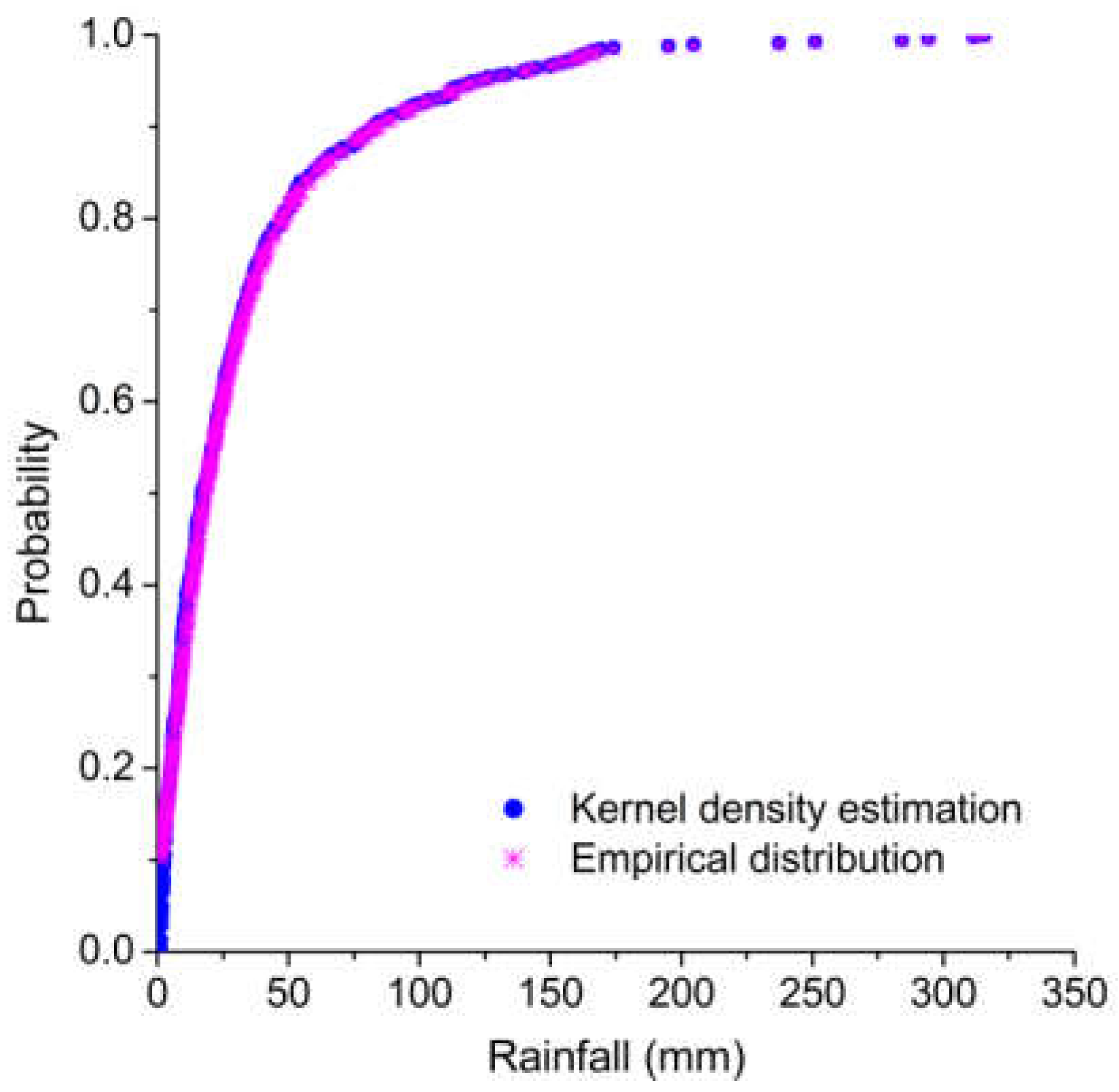
| Variate | Typhoon | Rainfall | Storm Surge |
|---|---|---|---|
| K–S statistic D | 0.017 | 0.066 | 0.011 |
| Pair | Gaussian Copula | Student’s t-Copula | Clayton Copula | Frank Copula | Gumbel Copula | |||||
|---|---|---|---|---|---|---|---|---|---|---|
| KS | AIC | KS | AIC | KS | AIC | KS | AIC | KS | AIC | |
| Typhoon–rainfall | 0.081 | −963.566 | 0.084 | −948.301 | 0.084 | −542.389 | 0.080 | −978.488 | 0.066 | −1169.123 |
| Typhoon–storm surge | 0.049 | −1047.931 | 0.046 | −1082.368 | 0.066 | −726.048 | 0.051 | −1030.418 | 0.040 | −1274.238 |
| Rainfall–storm surge | 0.086 | −815.687 | 0.085 | −837.389 | 0.085 | −570.130 | 0.085 | −825.573 | 0.064 | −971.122 |
| Distribution | Gaussian Copula | Student’s t Copula | Gumbel Copula |
|---|---|---|---|
| AIC | −925.276 | −901.062 | −957.371 |
| K–S | 0.068 | 0.069 | 0.057 |
| Return Period (Years) | 5 | 10 | 20 | 50 | 100 |
|---|---|---|---|---|---|
| 0.430 | 0.233 | 0.121 | 0.050 | 0.025 | |
| 0.053 | 0.024 | 0.011 | 0.004 | 0.002 | |
| 0.008 | 0.001 | 1.25 × 10⁻⁴ | 8 × 10⁻⁶ | 1 × 10⁻⁶ |
| RP (years) | Typhoon T | Rainfall H (mm) | Storm Surge Z (m) | P(H|T) | P(Z|T) | P(H,Z) | P(H,Z|T) |
|---|---|---|---|---|---|---|---|
| 5 | 0.65 | 46 | 2.67 | 0.434 | 0.334 | 0.069 | 0.266 |
| 10 | 0.74 | 80 | 2.82 | 0.375 | 0.258 | 0.027 | 0.239 |
| 20 | 0.81 | 125.6 | 2.95 | 0.345 | 0.221 | 0.012 | 0.229 |
| 50 | 0.9 | 210.7 | 3.1 | 0.328 | 0.198 | 0.004 | 0.225 |
| 100 | 0.96 | 294.2 | 3.21 | 0.322 | 0.191 | 0.002 | 0.223 |
| Year | Rainfall Events | Inundation Depth (m) | Economic Loss (Million Dollars) |
|---|---|---|---|
| 2008 | RE-1 | 1.5 | 51.72 |
| 2009 | RE-2 | 0.5 | 9.01 |
| RE-3 | 0.7 | 6.06 | |
| RE-4 | 0.5 | 4.74 |
| Return Period (Years) | 5 | 10 | 20 | 50 | 100 |
|---|---|---|---|---|---|
| P(H,Z) | 0.069 | 0.027 | 0.012 | 0.004 | 0.002 |
| P(H,Z|T) | 0.266 | 0.239 | 0.229 | 0.225 | 0.223 |
| Flood damage (million dollars) | 7.38 | 11.17 | 16.51 | 20.66 | 24.83 |
© 2018 by the authors. Licensee MDPI, Basel, Switzerland. This article is an open access article distributed under the terms and conditions of the Creative Commons Attribution (CC BY) license (http://creativecommons.org/licenses/by/4.0/).
Share and Cite
Xu, H.; Xu, K.; Bin, L.; Lian, J.; Ma, C. Joint Risk of Rainfall and Storm Surges during Typhoons in a Coastal City of Haidian Island, China. Int. J. Environ. Res. Public Health 2018, 15, 1377. https://doi.org/10.3390/ijerph15071377
Xu H, Xu K, Bin L, Lian J, Ma C. Joint Risk of Rainfall and Storm Surges during Typhoons in a Coastal City of Haidian Island, China. International Journal of Environmental Research and Public Health. 2018; 15(7):1377. https://doi.org/10.3390/ijerph15071377
Chicago/Turabian StyleXu, Hongshi, Kui Xu, Lingling Bin, Jijian Lian, and Chao Ma. 2018. "Joint Risk of Rainfall and Storm Surges during Typhoons in a Coastal City of Haidian Island, China" International Journal of Environmental Research and Public Health 15, no. 7: 1377. https://doi.org/10.3390/ijerph15071377
APA StyleXu, H., Xu, K., Bin, L., Lian, J., & Ma, C. (2018). Joint Risk of Rainfall and Storm Surges during Typhoons in a Coastal City of Haidian Island, China. International Journal of Environmental Research and Public Health, 15(7), 1377. https://doi.org/10.3390/ijerph15071377