Assessing the Impact of Urbanization on Direct Runoff Using Improved Composite CN Method in a Large Urban Area


Abstract
1. Introduction
2. Materials and Methods
2.1. Study Area and Data
2.2. Direct Runoff Simulation Method
2.3. Linear Spectral Mixture Analysis
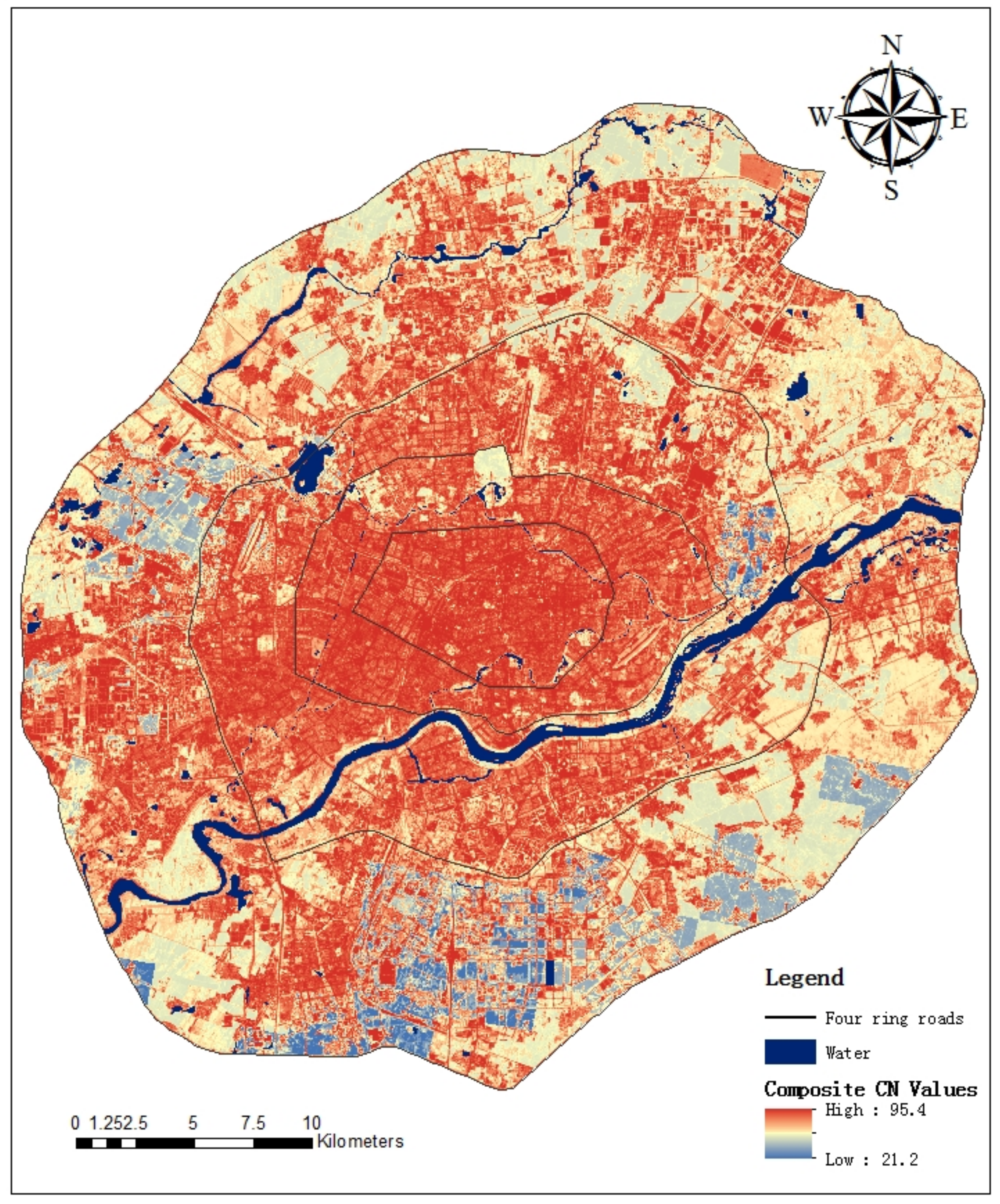
2.4. Improved Composite CN Method
2.5. Trend and Risk Analysis for Direct Runoff
3. Results and Discussion
3.1. LSMA Accuracy Assessment
3.2. Direct Runoff Volume and Risk
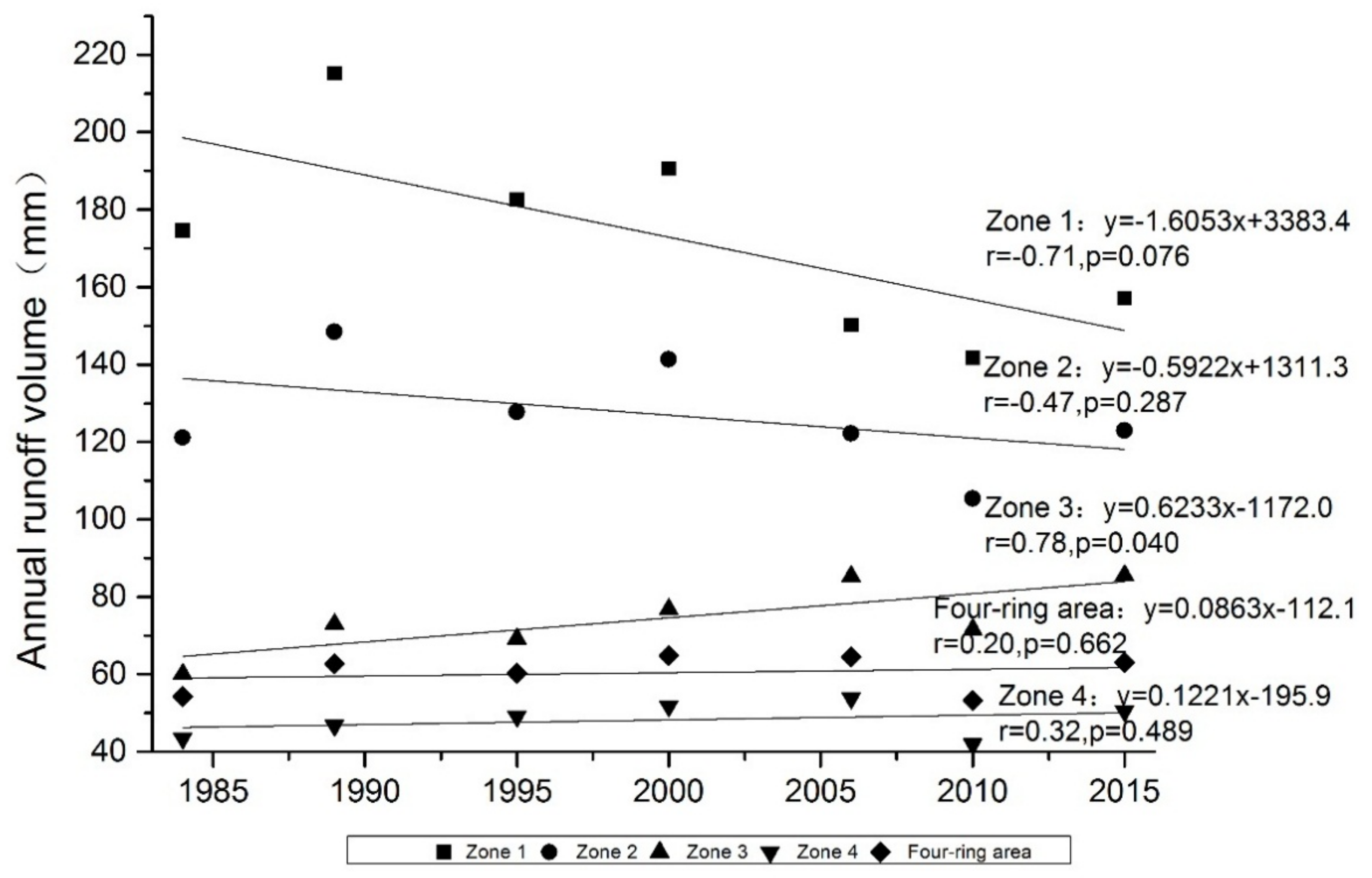
3.3. Variation Trends of Direct Runoff at Regional Scale
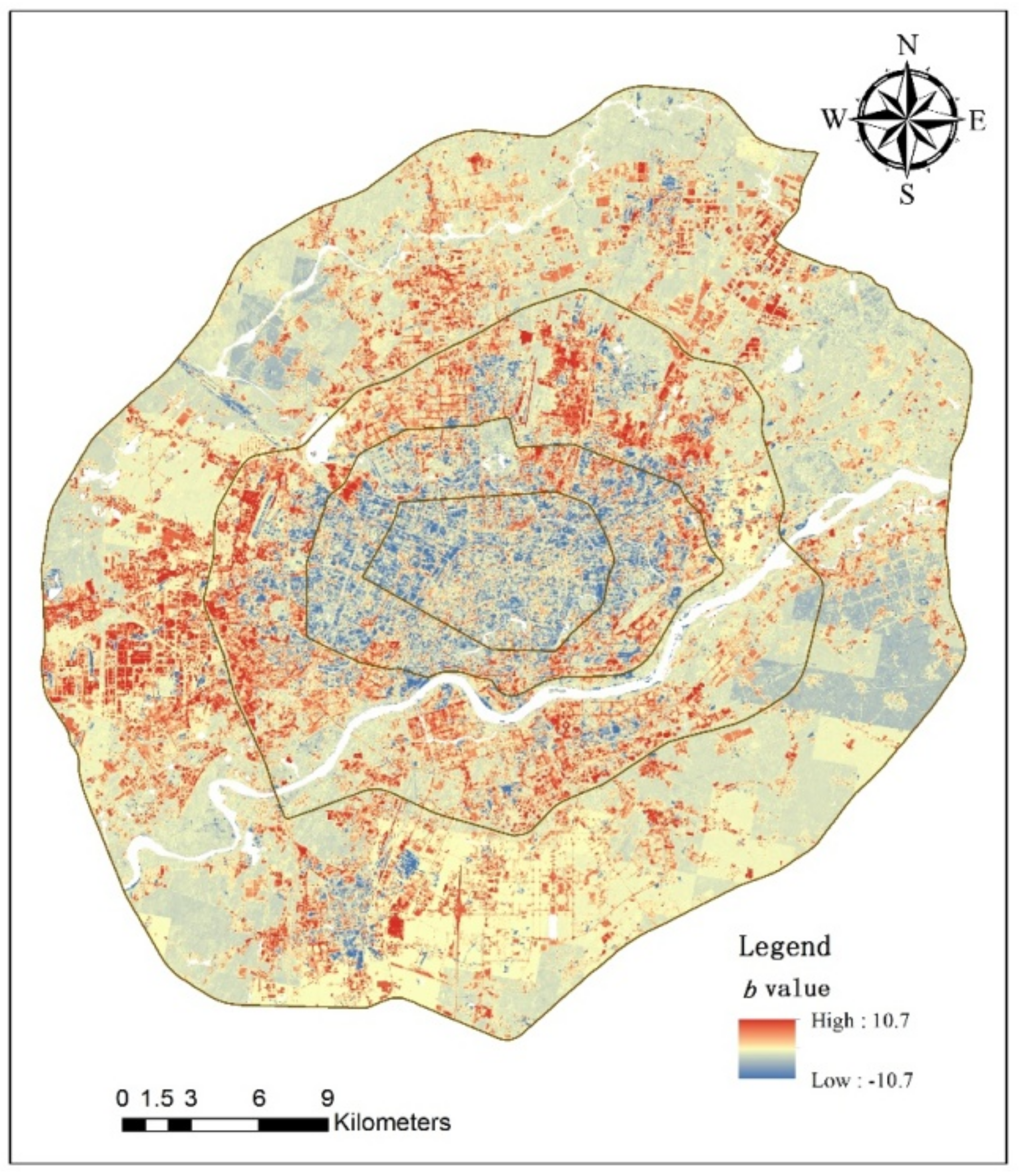
3.4. Trends of Direct Runoff at Pixel Scale
3.4.1. Trend and Extent
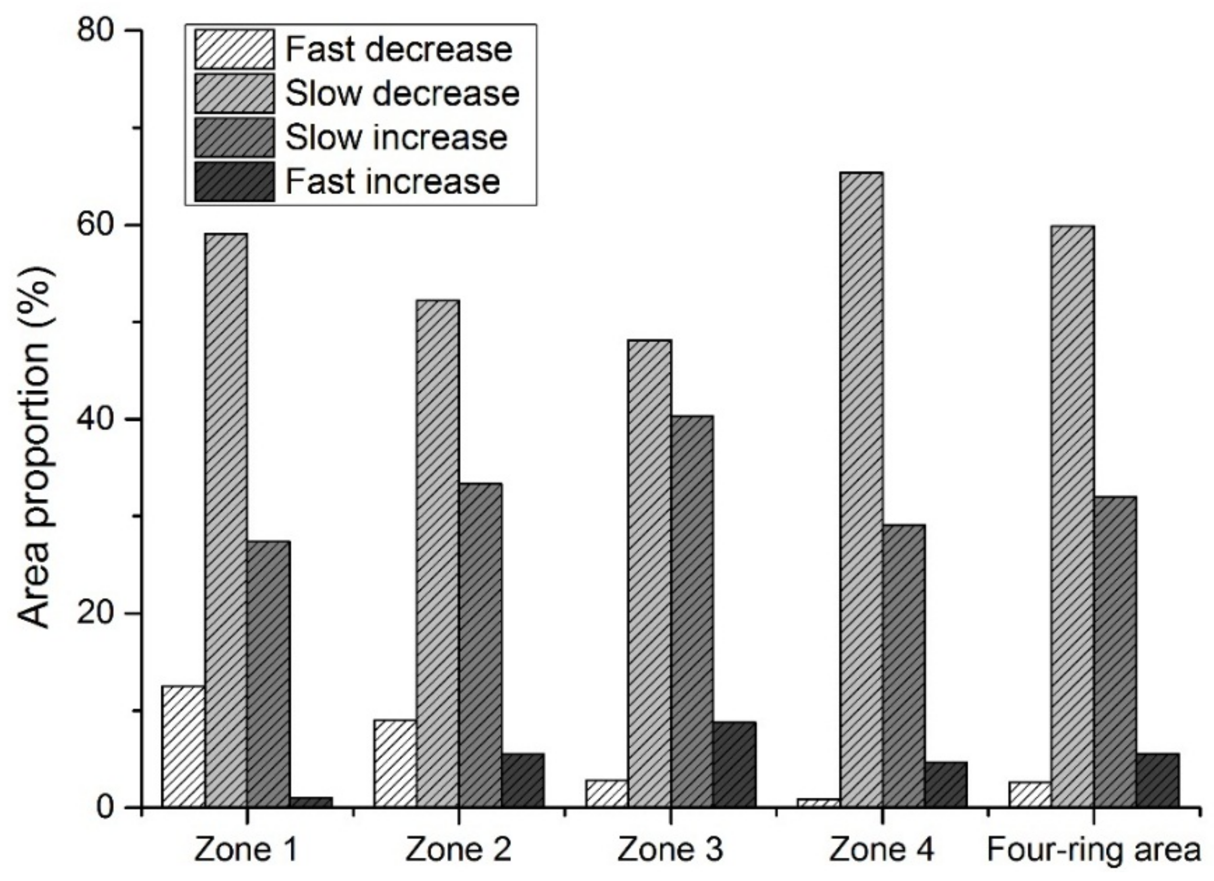
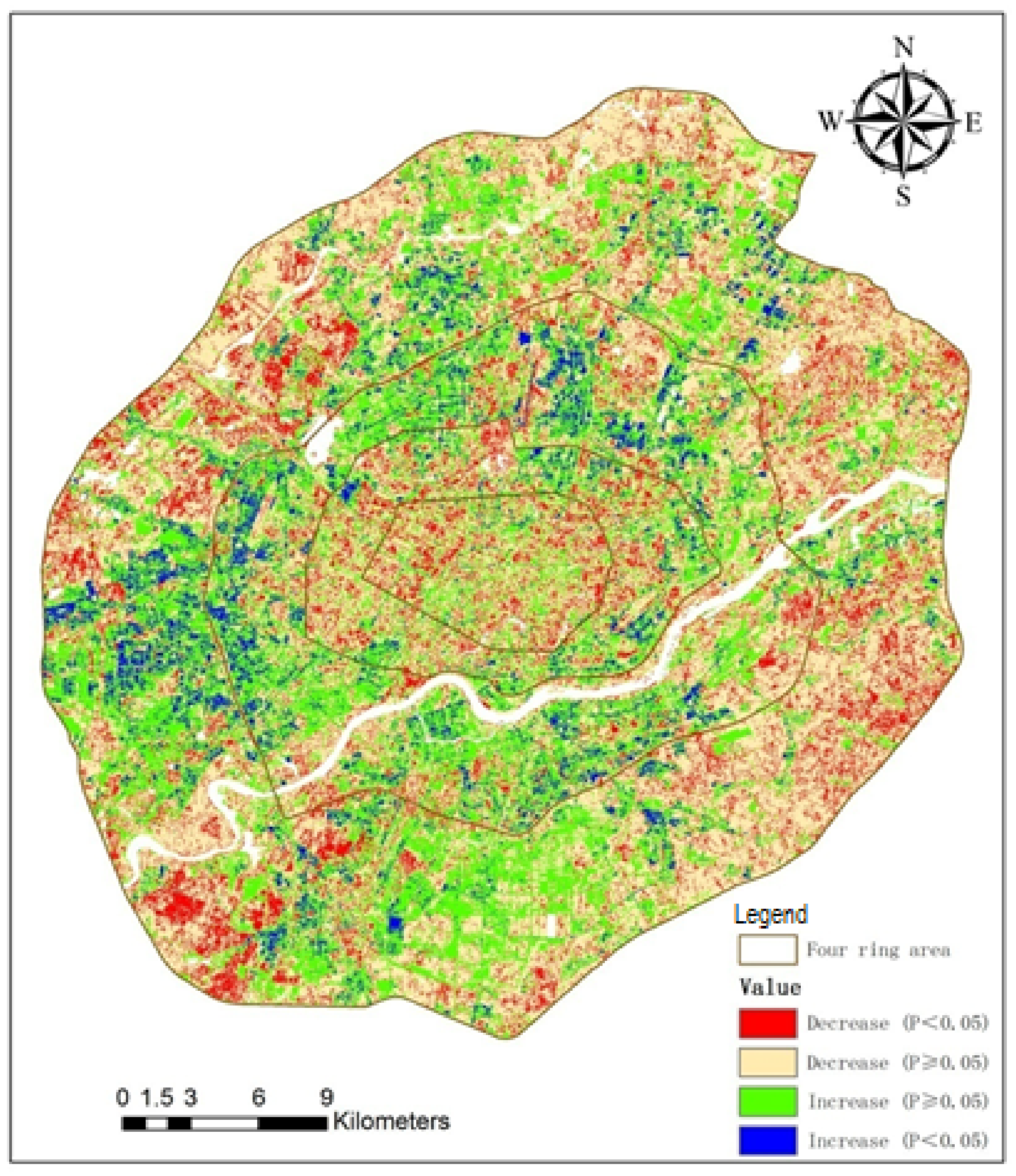
3.4.2. Significance Level Analysis
4. Conclusions
Acknowledgments
Author Contributions
Conflicts of Interest
References
- Miller, J.D.; Kim, H.; Kjeldsen, T.R.; Packman, J.; Grebby, S.; Dearden, R. Assessing the impact of urbanization on storm runoff in a peri-urban catchment using historical change in Impervious Cover. J. Hydrol. 2014, 515, 59–70. [Google Scholar] [CrossRef]
- Du, S.Q.; Van Rompaey, A.; Shi, P.J.; Wang, J.A. A dual effect of urban expansion on flood risk in the Pearl River Delta (China) revealed by land-use scenarios and direct runoff simulation. Nat. Hazards 2015, 77, 111–128. [Google Scholar] [CrossRef]
- Richert, E.; Bianchin, S.; Heilmeier, H.; Merta, M.; Seidler, C. A method for linking results from an evaluation of land use scenarios from the viewpoint of flood prevention and nature conservation. Landsc. Urban Plan. 2011, 103, 118–128. [Google Scholar] [CrossRef]
- Li, C.; Liu, M.; Hu, Y.; Gong, J.; Xu, Y. Modeling the quality and quantity of runoff in a highly urbanized catchment using storm water management model. Pol. J. Environ. Stud. 2016, 25, 1573–1581. [Google Scholar] [CrossRef]
- Wu, C.; Chau, K. A flood forecasting neural network model with genetic algorithm. Int. J. Environ. Pollut. 2006, 28, 261–273. [Google Scholar] [CrossRef]
- Walega, A.; Rutkowska, A.; Grzebinoga, M. Direct runoff assessment using modified SME method in catchments in the Upper Vistula River Basin. Acta Geophys. 2017, 65, 363–375. [Google Scholar] [CrossRef]
- Singh, P.K.; Yaduvanshi, B.K.; Patel, S.; Ray, S. SCS-CN based quantification of potential of rooftop catchments and computation of ASRC for rainwater harvesting. Water Resour. Manag. 2013, 27, 2001–2012. [Google Scholar] [CrossRef]
- Bartlett, M.S.; Parolari, A.J.; Mcdonnell, J.J.; Porporato, A. Beyond the SCS-CN method: A theoretical framework for spatially lumped rainfall-runoff response. Water Resour. Res. 2016, 52, 4608–4627. [Google Scholar] [CrossRef]
- Golding, B.L.; Smith, R.E.; Willeke, G.E.; Ponce, V.M.; Hawkins, R.H. Runoff curve number: Has it reached maturity? J. Hydrol. Eng. 1997, 2, 145–148. [Google Scholar] [CrossRef]
- Bonan, G. Ecological Climatology: Concepts and Applications; Cambridge University Press: Cambridge, UK, 2015. [Google Scholar]
- Yao, L.; Chen, L.D.; Wei, W.; Sun, R.H. Potential reduction in urban runoff by Green Spaces in Beijing: A scenario analysis. Urban For. Urban Green. 2015, 14, 300–308. [Google Scholar] [CrossRef]
- Mileti, D. Disasters by Design: A Reassessment of Natural Hazards in the United States; Joseph Henry Press: Washington, DC, USA, 1999. [Google Scholar]
- Maharjan, B.; Pachel, K.; Loigu, E. Modelling stormwater runoff, quality, and pollutant loads in a large urban catchment. Proc. Est. Acad. Sci. 2017, 66, 225–242. [Google Scholar] [CrossRef]
- Ebrahimian, A.; Gulliver, J.S.; Wilson, B.N. Effective impervious area for runoff in Urban Watersheds. Hydrol. Process. 2016, 30, 3717–3729. [Google Scholar] [CrossRef]
- Zhang, B.A.; Xie, G.D.; Zhang, C.Q.; Zhang, J. The economic benefits of rainwater-runoff reduction by urban green spaces: A case study in Beijing, China. J. Environ. Manag. 2012, 100, 65–71. [Google Scholar] [CrossRef] [PubMed]
- Brezonik, P.L.; Stadelmann, T.H. Analysis and predictive models of stormwater runoff volumes, loads, and pollutant concentrations from watersheds in the twin cities metropolitan area, Minnesota, USA. Water Res. 2002, 36, 1743–1757. [Google Scholar] [CrossRef]
- Fan, F.; Deng, Y.; Hu, X.; Weng, Q. Estimating composite curve number using an improved SCS-CN method with remotely sensed variables in Guangzhou, China. Remote Sens. 2013, 5, 1425–1438. [Google Scholar] [CrossRef]
- Taormina, R.; Chau, K.-W.; Sivakumar, B. Neural network river forecasting through baseflow separation and binary-coded swarm optimization. J. Hydrol. 2015, 529, 1788–1797. [Google Scholar] [CrossRef]
- Gholami, V.; Chau, K.; Fadaee, F.; Torkaman, J.; Ghaffari, A. Modeling of groundwater level fluctuations using dendrochronology in alluvial aquifers. J. Hydrol. 2015, 529, 1060–1069. [Google Scholar] [CrossRef]
- Wang, W.-C.; Xu, D.-M.; Chau, K.-W.; Lei, G.-J. Assessment of river water quality based on theory of variable fuzzy sets and fuzzy binary comparison method. Water Resour. Manag. 2014, 28, 4183–4200. [Google Scholar] [CrossRef]
- Jiao, P.J.; Xu, D.; Wang, S.L.; Yu, Y.D.; Han, S.J. Improved scs-cn method based on storage and depletion of antecedent daily precipitation. Water Resour. Manag. 2015, 29, 4753–4765. [Google Scholar] [CrossRef]
- Hawkins, R.H. Curve number method: Time to think anew? J. Hydrol. Eng. 2014, 19, 1059. [Google Scholar] [CrossRef]
- Ponce, V.M.; Hawkins, R.H. Runoff curve number: Has it reached maturity? J. Hydrol. Eng. 1996, 1, 11–19. [Google Scholar] [CrossRef]
- Patil, J.; Sarangi, A.; Singh, O.; Singh, A.; Ahmad, T. Development of a GIS interface for estimation of runoff from watersheds. Water Resour. Manag. 2008, 22, 1221–1239. [Google Scholar] [CrossRef]
- Dong, L.H.; Xiong, L.H.; Lall, U.; Wang, J.W. The effects of land use change and precipitation change on direct runoff in Wei River Watershed, China. Water Sci. Technol. 2015, 71, 289–295. [Google Scholar] [CrossRef] [PubMed]
- Randhir, T.O.; Tsvetkova, O. Spatiotemporal dynamics of landscape pattern and hydrologic process in watershed systems. J. Hydrol. 2011, 404, 1–12. [Google Scholar] [CrossRef]
- Huang, M.B.; Gallichand, J.; Wang, Z.L.; Goulet, M. A modification to the soil conservation service curve number method for steep slopes in the Loess Plateau of China. Hydrol. Process. 2006, 20, 579–589. [Google Scholar] [CrossRef]
- Patil, J.P.; Sarangi, A.; Singh, A.K.; Ahmad, T. Evaluation of modified CN methods for watershed runoff estimation using a GIS-based interface. Biosyst. Eng. 2008, 100, 137–146. [Google Scholar] [CrossRef]
- Liu, M.; Li, C.; Hu, Y.; Sun, F.; Xu, Y.; Chen, T. Combining clue-s and swat models to forecast land use change and non-point source pollution impact at a watershed scale in Liaoning province, China. Chin. Geogr. Sci. 2013, 24, 540–550. [Google Scholar] [CrossRef]
- Chen, X.; Chau, K.; Busari, A. A comparative study of population-based optimization algorithms for downstream river flow forecasting by a hybrid neural network model. Eng. Appl. Artif. Intell. 2015, 46, 258–268. [Google Scholar] [CrossRef]
- Chau, K. A split-step particle swarm optimization algorithm in river stage forecasting. J. Hydrol. 2007, 346, 131–135. [Google Scholar] [CrossRef]
- Tirkey, A.S.; Pandey, A.C.; Nathawat, M.S. Use of high-resolution satellite data, GIS and NRCS-CN technique for the estimation of rainfall-induced run-off in small catchment of Jharkhand India. Geocarto Int. 2014, 29, 778–791. [Google Scholar] [CrossRef]
- Goldshleger, N.; Maor, A.; Garzuzi, J.; Asaf, L. Influence of land use on the quality of runoff along Israel’s coastal strip (demonstrated in the cities of Herzliya and Ra’anana). Hydrol. Process. 2015, 29, 1289–1300. [Google Scholar] [CrossRef]
- Rejani, R.; Rao, K.V.; Osman, M.; Chary, G.R.; Reddy, K.S.; Rao, C.S. Spatial and temporal estimation of runoff in a semi-arid Microwatershed of Southern India. Environ. Monit. Assess. 2015, 187. [Google Scholar] [CrossRef] [PubMed]
- Li, C.; Liu, M.; Hu, Y.; Gong, J.; Sun, F.; Xu, Y. Characterization and first flush analysis in road and roof runoff in Shenyang, China. Water Sci. Technol. 2014, 70, 397–406. [Google Scholar] [CrossRef] [PubMed]
- Ridd, M.K. Exploring a V-I-S (vegetation-impervious-soil) model for urban ecosystem analysis through remote sensing: Comparative anatomy for citiest. Int. J. Remote Sens. 1995, 16, 2165–2185. [Google Scholar] [CrossRef]
- Silveira, L.; Charbonnier, F.; Genta, J.L. The antecedent soil moisture condition of the curve number procedure. Hydrol. Sci. J. 2000, 45, 3–12. [Google Scholar] [CrossRef]
- Sahu, R.K.; Mishra, S.K.; Eldho, T.I. An improved AMC-coupled runoff curve number model. Hydrol. Process. 2010, 24, 2834–2839. [Google Scholar] [CrossRef]
- Mishra, S.K.; Singh, V.P.; Singh, V.P.; Frevert, D. SCS-CN-based hydrologic simulation package. In Mathematical Models in Small Watershed Hydrology and Applications; Water Resources Publications: Saint Joseph County, IN, USA, 2002; pp. 391–464. [Google Scholar]
- Roberts, D.A.; Gardner, M.; Church, R.; Ustin, S.; Scheer, G.; Green, R.O. Mapping chaparral in the santa monica mountains using multiple endmember spectral mixture models. Remote Sens. Environ. 1998, 65, 267–279. [Google Scholar] [CrossRef]
- Adams, J.B.; Sabol, D.E.; Kapos, V.; Almeida, R.; Roberts, D.A.; Smith, M.O.; Gillespie, A.R. Classification of multispectral images based on fractions of endmembers–application to land-cover change in the Brazilian Amazon. Remote Sens. Environ. 1995, 52, 137–154. [Google Scholar] [CrossRef]
- Smith, M.O.; Ustin, S.L.; Adams, J.B.; Gillespie, A.R. Vegetation in deserts. 1. A regional measure of abundance from multispectral images. Remote Sens. Environ. 1990, 31, 1–26. [Google Scholar] [CrossRef]
- Yang, J.; He, Y. Automated mapping of impervious surfaces in urban and suburban areas: Linear spectral unmixing of high spatial resolution imagery. Int. J. Appl. Earth Obs. Geoinf. 2017, 54, 53–64. [Google Scholar] [CrossRef]
- Xu, J.; Zhao, Y.; Zhong, K.; Ruan, H.; Liu, X. Coupling modified linear spectral mixture analysis and soil conservation service curve number (SCS-CN) models to simulate surface runoff: Application to the main urban area of Guangzhou, China. Water 2016, 8, 550. [Google Scholar] [CrossRef]
- Angrill, S.; Petit-Boix, A.; Morales-Pinzón, T.; Josa, A.; Rieradevall, J.; Gabarrell, X. Urban rainwater runoff quantity and quality—A potential endogenous resource in cities? J. Environ. Manag. 2017, 189, 14–21. [Google Scholar] [CrossRef] [PubMed]
- Suribabu, C.R.; Bhaskar, J. Evaluation of urban growth effects on surface runoff using SCS-CN method and Green-Ampt infiltration model. Earth Sci. Inform. 2015, 8, 609–626. [Google Scholar] [CrossRef]
- Qin, H.-P.; He, K.-M.; Fu, G. Modeling middle and final flush effects of urban runoff pollution in an urbanizing catchment. J. Hydrol. 2016, 534, 638–647. [Google Scholar] [CrossRef]


| Vegetation Type | NDVI Range | CNV | ||||
|---|---|---|---|---|---|---|
| A | B | C | D | |||
| Vegetated | Good Condition | NDVI ≥ 0.7 | 21 | 41 | 55 | 63 |
| Fair Condition | 0.4 ≤ NDVI < 0.7 | 30 | 50 | 62 | 68 | |
| Poor Condition | 0 ≤ NDVI < 0.4 | 48 | 62 | 72 | 76 | |
| Non-Vegetated | NDVI < 0 | 59 | 72 | 80 | 85 | |
| Soil Type | Soil Texture | CNS |
|---|---|---|
| A | Sand ≥ 50% and clay ≤ 10% | 59 |
| B | Sand ≥ 50% and clay > 10% | 72 |
| C | Sand < 50% and clay ≤ 40% | 80 |
| D | Sand < 50% and clay > 40% | 85 |
| Zones | 1984 | 1989 | 1995 | 2000 | 2006 | 2010 | 2015 |
|---|---|---|---|---|---|---|---|
| Zone 1 | 165.32 | 208.79 | 175.7 | 182.19 | 137.89 | 134.20 | 148.41 |
| Zone 2 | 109.86 | 139.17 | 119.17 | 131.94 | 110.18 | 97.40 | 113.66 |
| Zone 3 | 55.12 | 68.35 | 64.01 | 71.13 | 76.64 | 66.30 | 78.50 |
| Zone 4 | 41.55 | 45.23 | 47.07 | 49.85 | 49.65 | 39.51 | 45.51 |
| Four-ring area | 54.79 | 64.21 | 61.57 | 66.27 | 64.01 | 53.86 | 62.40 |
| Zones | 1984 | 1989 | 1995 | 2000 | 2006 | 2010 | 2015 |
|---|---|---|---|---|---|---|---|
| Zone 1 | 6.97 | 8.80 | 7.41 | 7.68 | 5.81 | 5.66 | 6.26 |
| Zone 2 | 9.51 | 12.05 | 10.32 | 11.43 | 9.54 | 8.44 | 9.84 |
| Zone 3 | 13.95 | 17.30 | 16.20 | 18.00 | 19.40 | 16.78 | 19.87 |
| Zone 4 | 33.18 | 36.12 | 37.59 | 39.81 | 39.65 | 31.55 | 36.34 |
| Four-ring area | 63.62 | 74.28 | 71.52 | 76.92 | 74.41 | 62.43 | 72.31 |
| Zones | Low Runoff Risk | Medium Runoff Risk | High Runoff Risk | Extremely High Runoff Risk | ||||
|---|---|---|---|---|---|---|---|---|
| Area in 2015 | Area Change (2015–1984) | Area in 2015 | Area Change (2015–1984) | Area in 2015 | Area Change (2015–1984) | Area in 2015 | Area Change (2015–1984) | |
| Zone 1 | 19.68 | 3.80 | 10.46 | −0.14 | 11.11 | 0.03 | 14.93 | −3.69 |
| Zone 2 | 55.31 | −7.43 | 16.44 | 7.82 | 13.85 | 6.12 | 17.37 | −6.52 |
| Zone 3 | 197.20 | −53.51 | 27.42 | 21.63 | 20.78 | 16.52 | 32.82 | 15.37 |
| Zone 4 | 632.22 | −93.78 | 38.04 | 32.51 | 25.63 | 22.28 | 54.35 | 39.00 |
| Four−ring area | 904.40 | −150.92 | 92.36 | 61.80 | 71.37 | 44.95 | 119.47 | 44.18 |
| Area | Decrease Ratio (p < 0.05) | Decrease Ratio (p ≥ 0.05) | Increase Ratio (p ≥ 0.05) | Increase Ratio (p < 0.05) |
|---|---|---|---|---|
| Zone 1 | 20.69 | 50.89 | 25.98 | 2.44 |
| Zone 2 | 16.81 | 44.39 | 32.09 | 6.70 |
| Zone 3 | 10.96 | 40.00 | 39.04 | 10.00 |
| Zone 4 | 15.28 | 50.95 | 28.60 | 5.16 |
| Four-ring area | 14.66 | 47.82 | 31.22 | 6.30 |
© 2018 by the authors. Licensee MDPI, Basel, Switzerland. This article is an open access article distributed under the terms and conditions of the Creative Commons Attribution (CC BY) license (http://creativecommons.org/licenses/by/4.0/).
Share and Cite
Li, C.; Liu, M.; Hu, Y.; Shi, T.; Zong, M.; Walter, M.T. Assessing the Impact of Urbanization on Direct Runoff Using Improved Composite CN Method in a Large Urban Area. Int. J. Environ. Res. Public Health 2018, 15, 775. https://doi.org/10.3390/ijerph15040775
Li C, Liu M, Hu Y, Shi T, Zong M, Walter MT. Assessing the Impact of Urbanization on Direct Runoff Using Improved Composite CN Method in a Large Urban Area. International Journal of Environmental Research and Public Health. 2018; 15(4):775. https://doi.org/10.3390/ijerph15040775
Chicago/Turabian StyleLi, Chunlin, Miao Liu, Yuanman Hu, Tuo Shi, Min Zong, and M. Todd Walter. 2018. "Assessing the Impact of Urbanization on Direct Runoff Using Improved Composite CN Method in a Large Urban Area" International Journal of Environmental Research and Public Health 15, no. 4: 775. https://doi.org/10.3390/ijerph15040775
APA StyleLi, C., Liu, M., Hu, Y., Shi, T., Zong, M., & Walter, M. T. (2018). Assessing the Impact of Urbanization on Direct Runoff Using Improved Composite CN Method in a Large Urban Area. International Journal of Environmental Research and Public Health, 15(4), 775. https://doi.org/10.3390/ijerph15040775