Coupling between Land–Ocean–Atmosphere and Pronounced Changes in Atmospheric/Meteorological Parameters Associated with the Hudhud Cyclone of October 2014


Abstract
1. Introduction
1.1. Hudhud
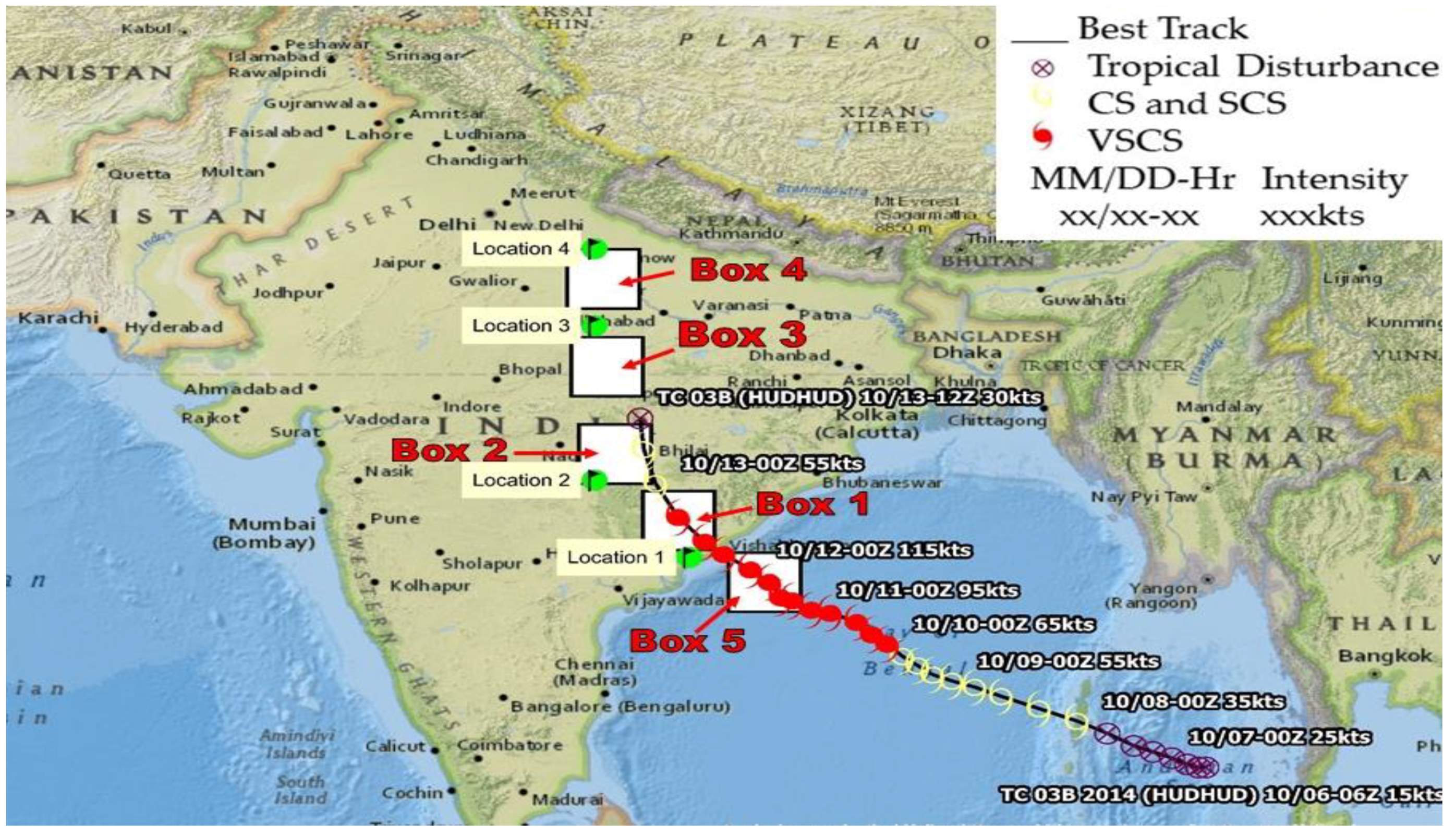
1.2. Study Area
2. Method and Materials
Data Used
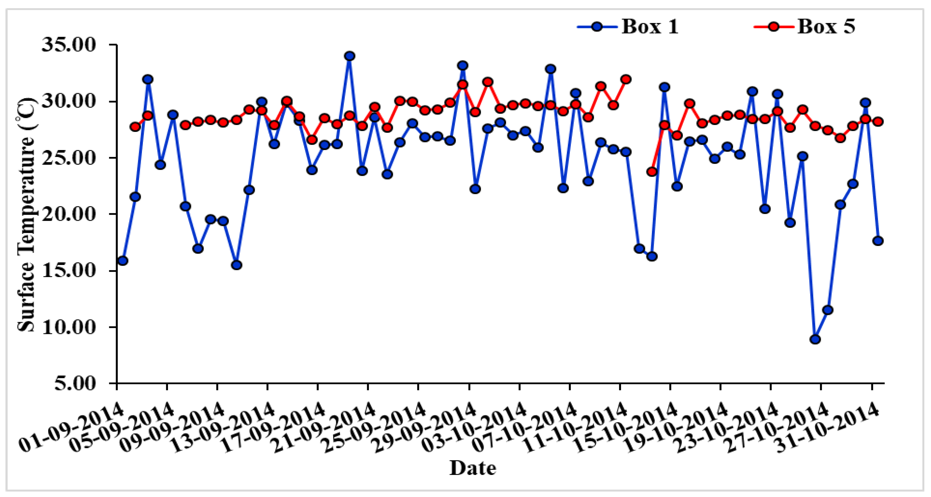
3. Results and Discussion
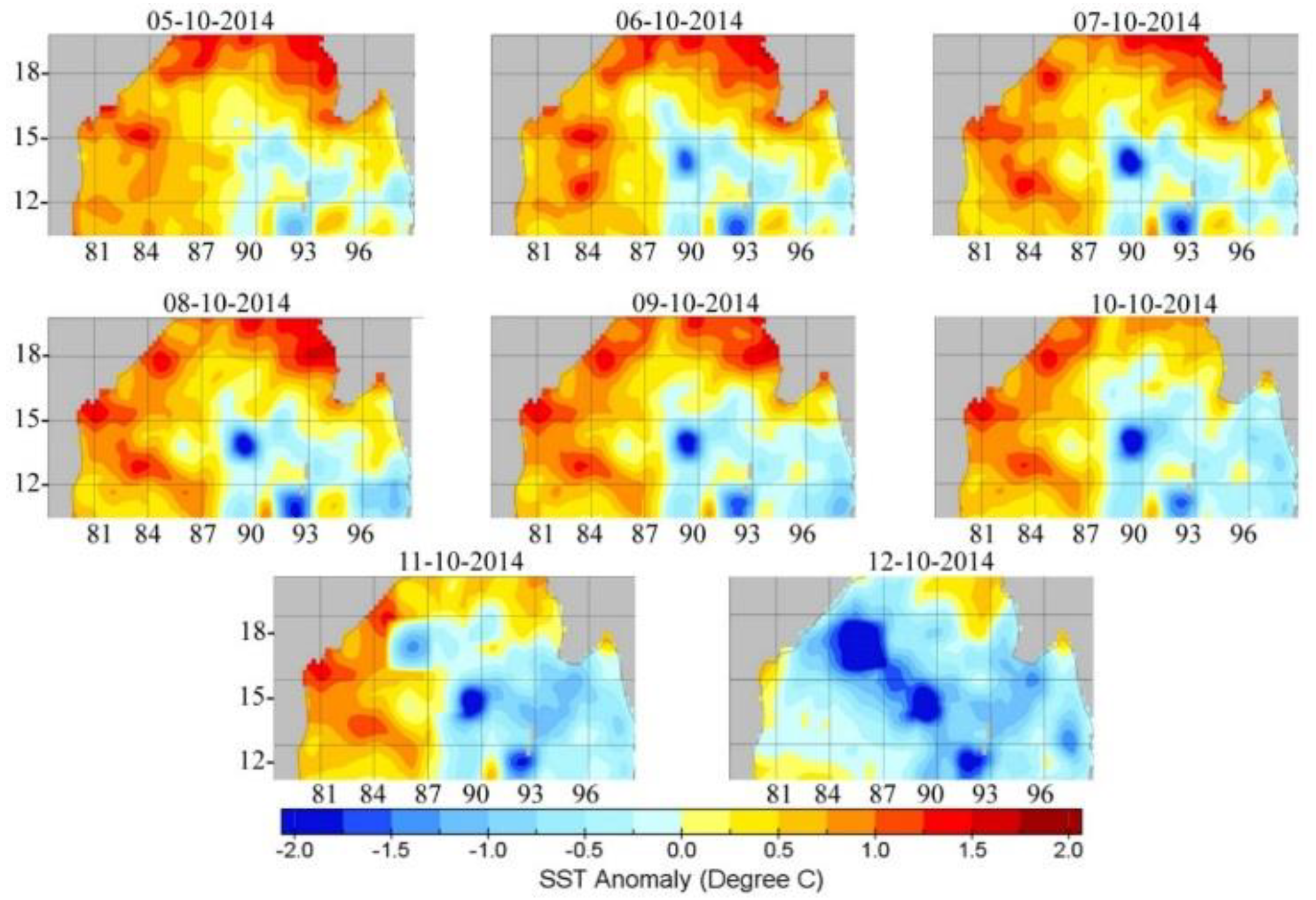
3.1. Spatio-Temporal Variability of SST Anomaly
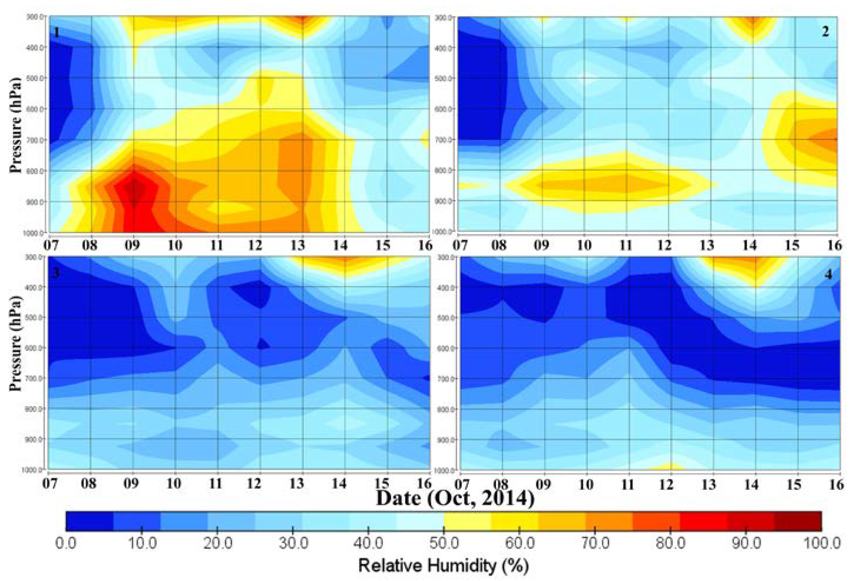
3.2. Relative Humidity
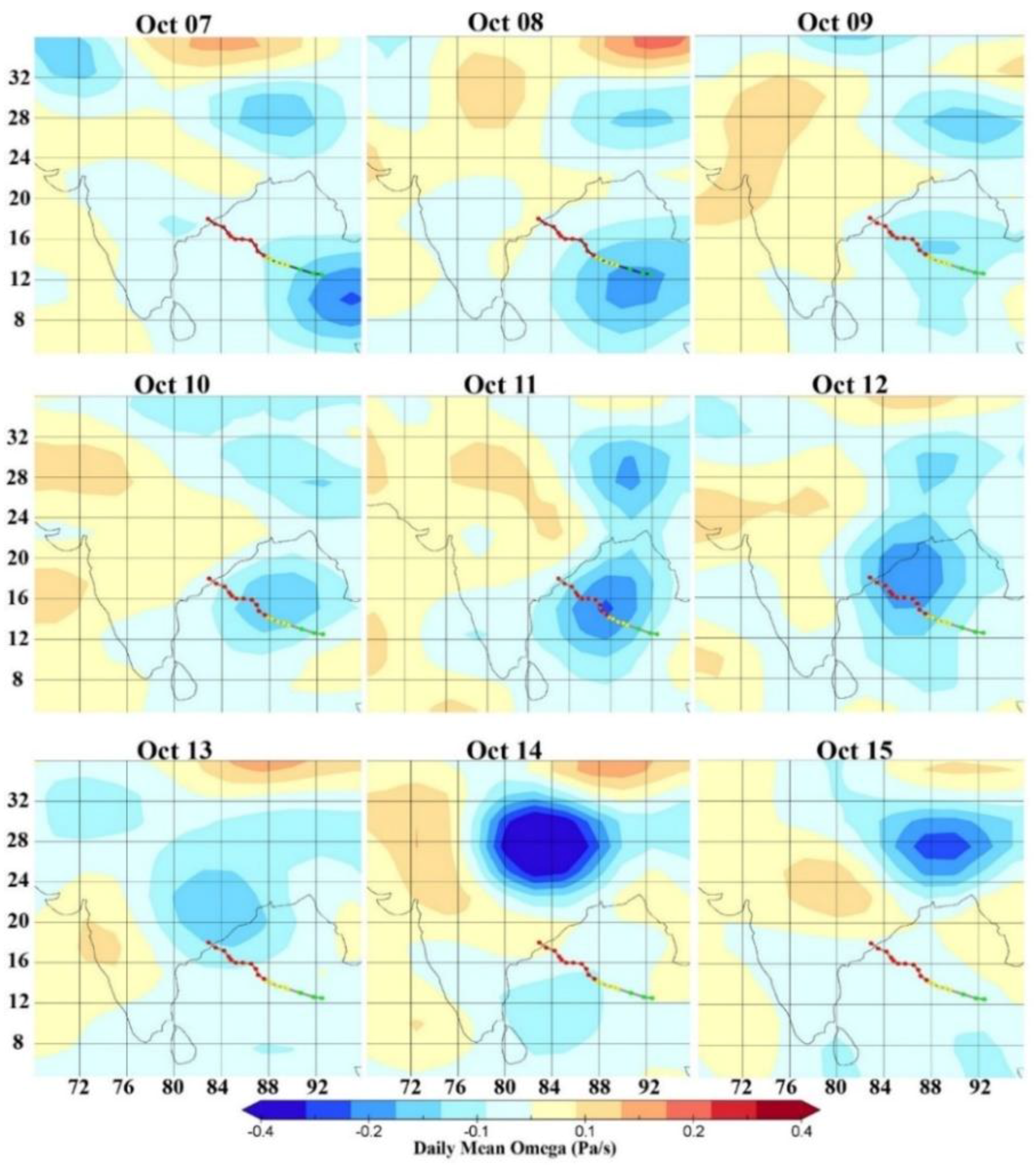
3.3. Omega
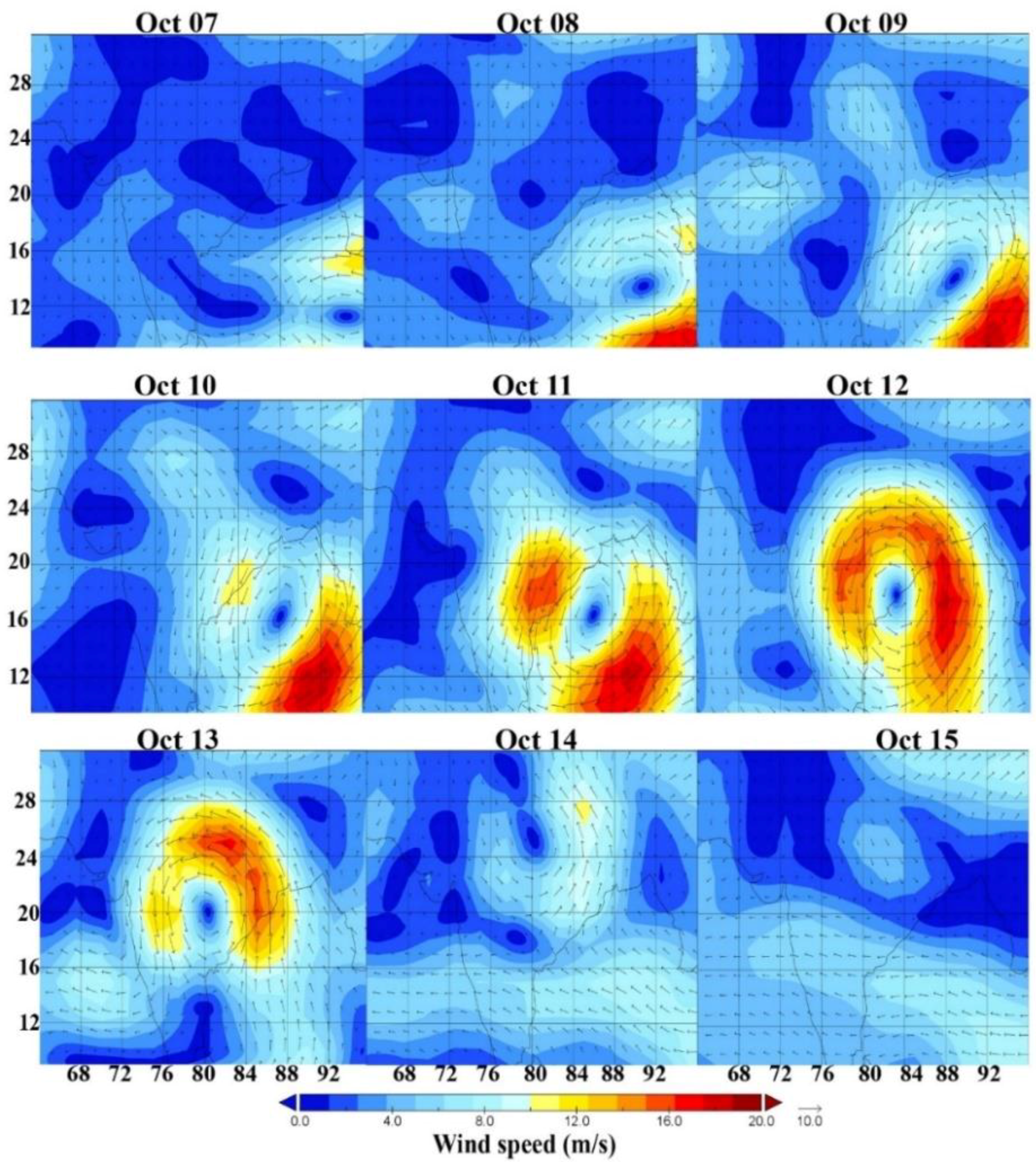
3.4. Wind Speed and Direction
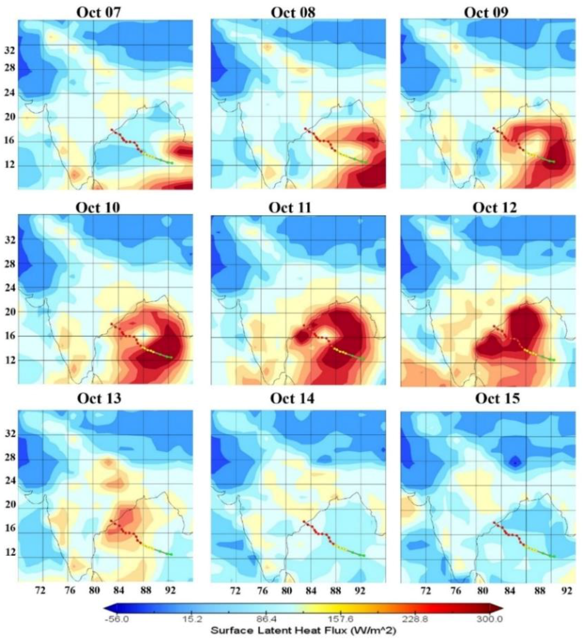
3.5. Surface Latent Heat Flux (SLHF)
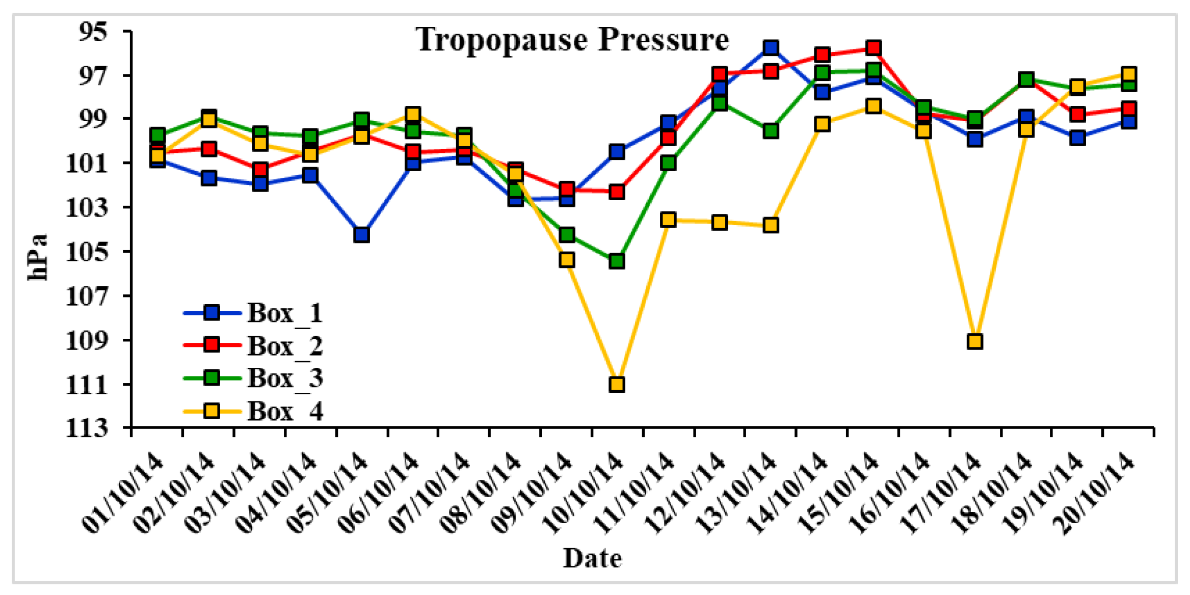
3.6. Tropopause Pressure
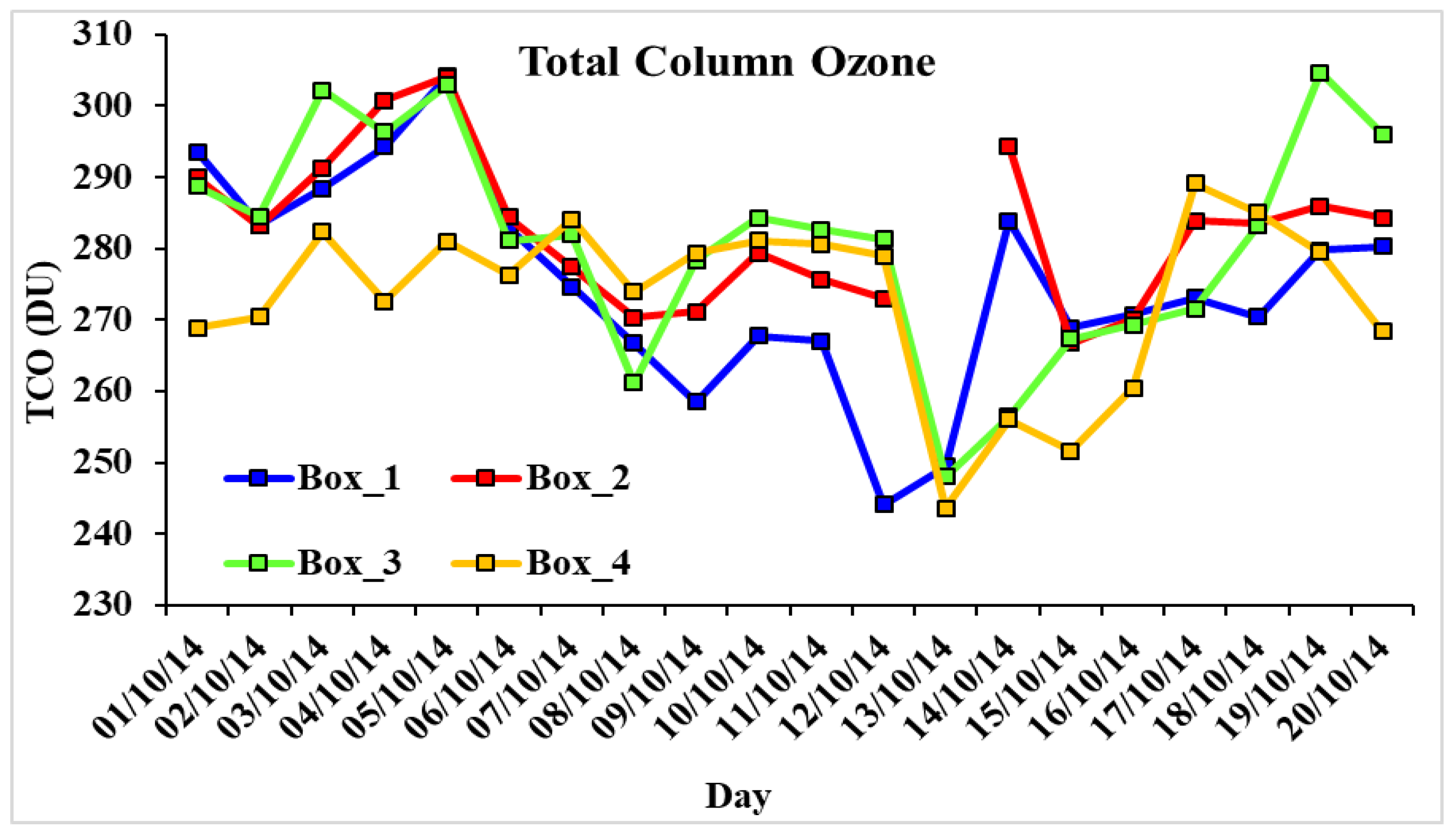
3.7. Total Column Ozone (TCO)
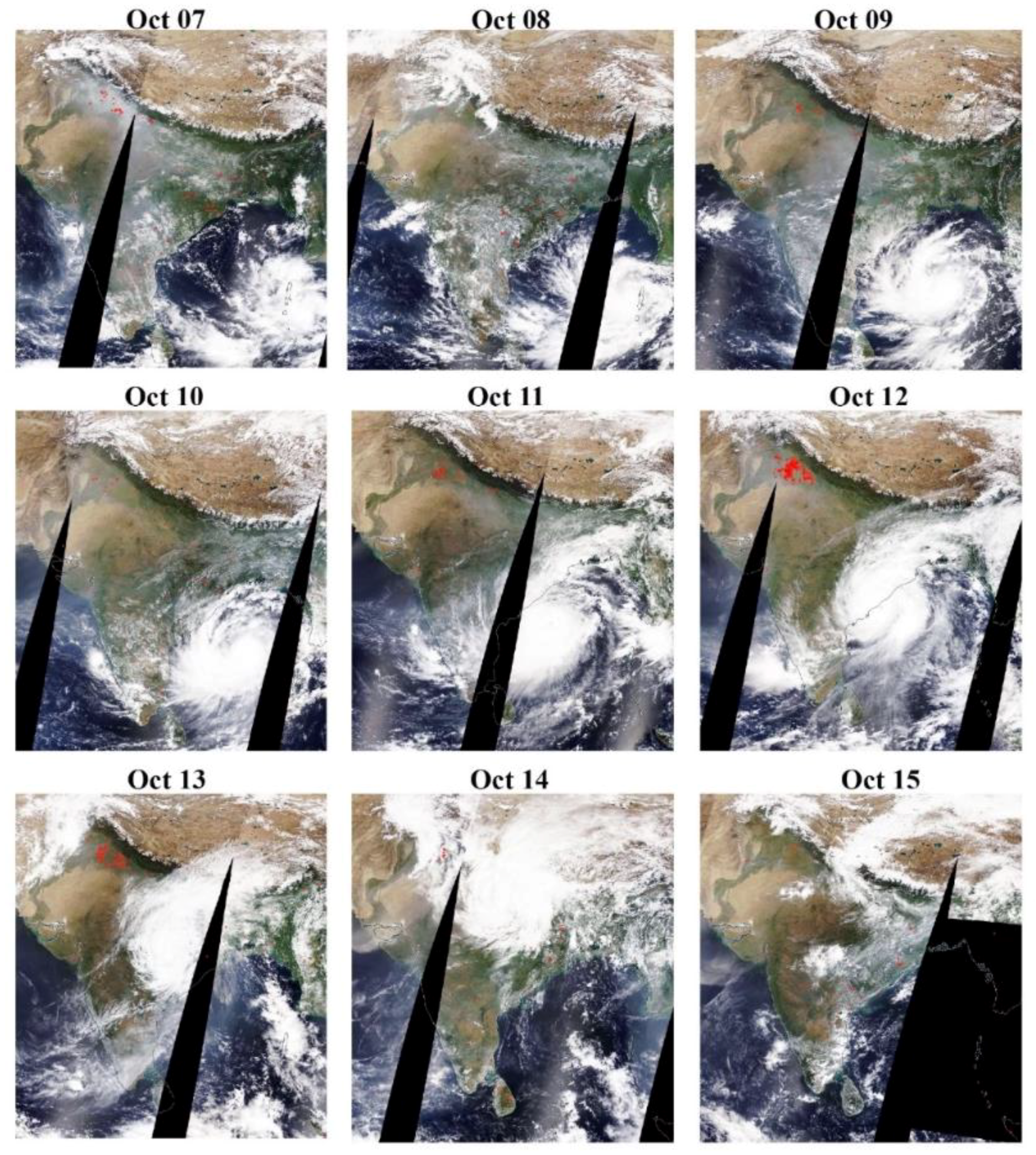
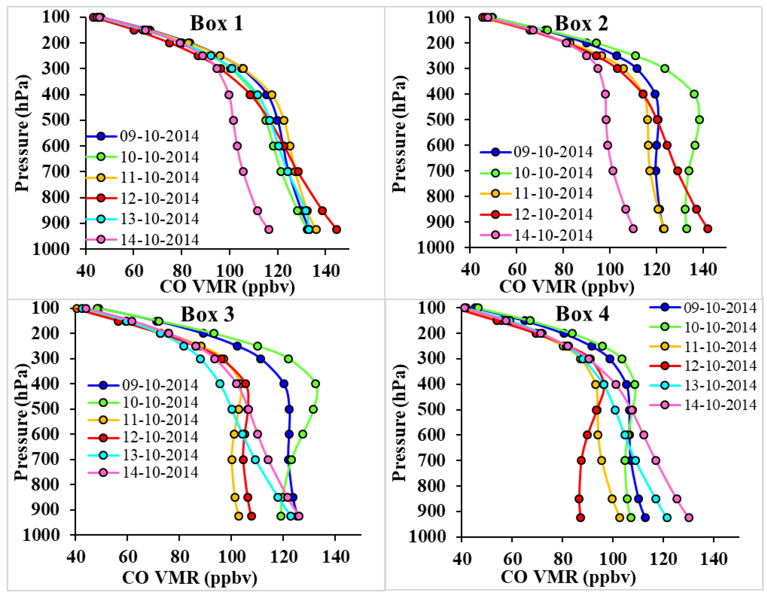
3.8. Variability of CO VMR
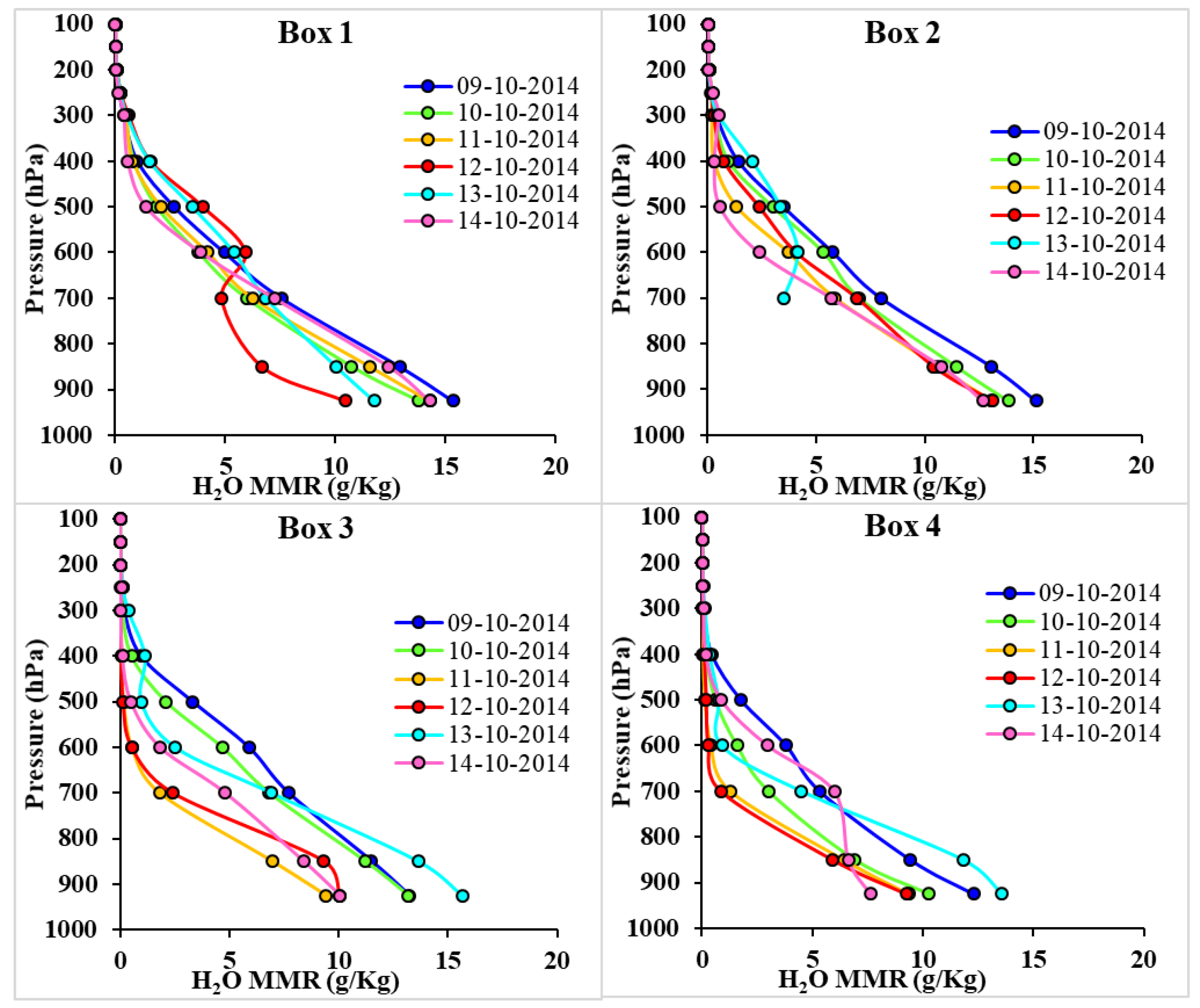
3.9. Variation of H2O MMR
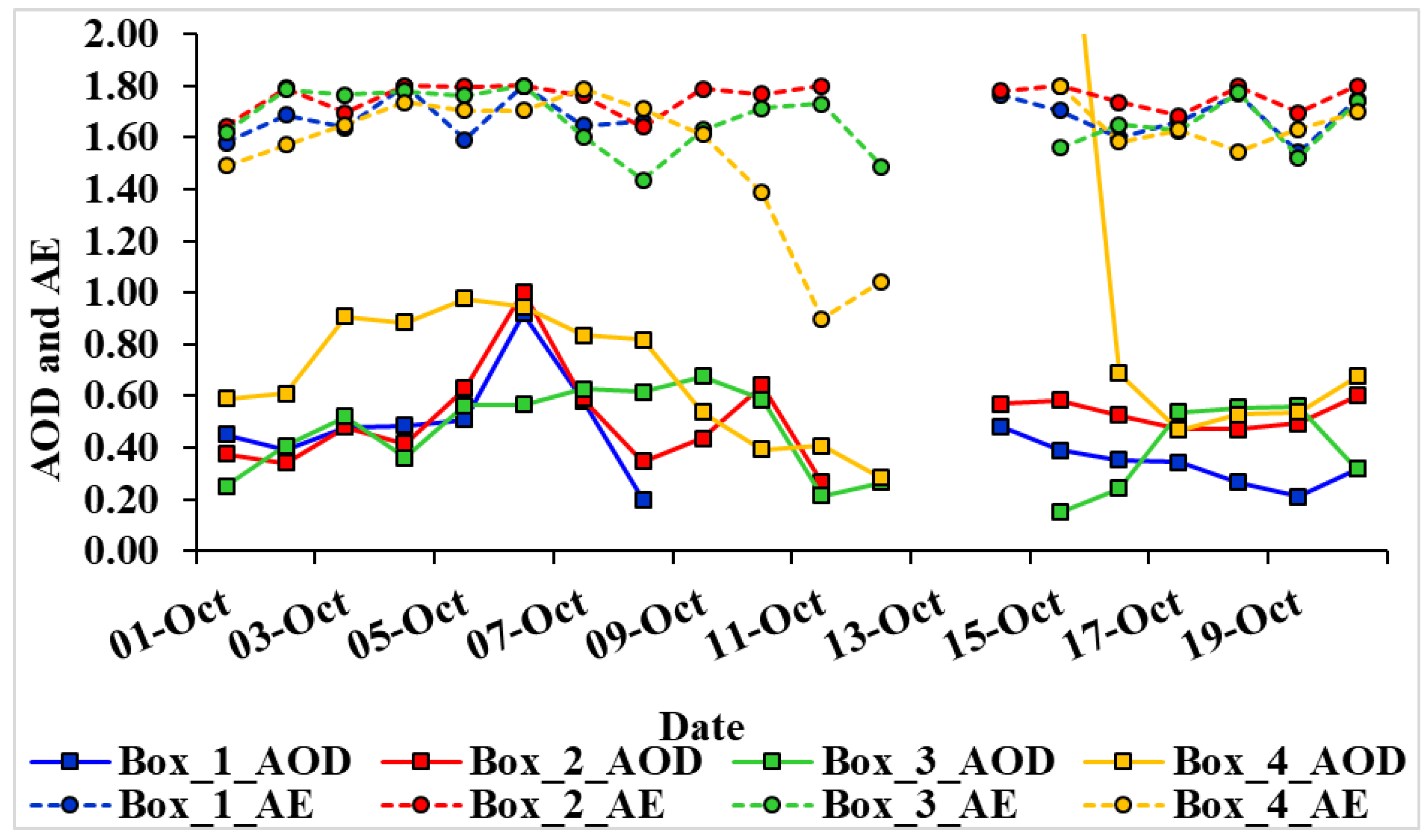
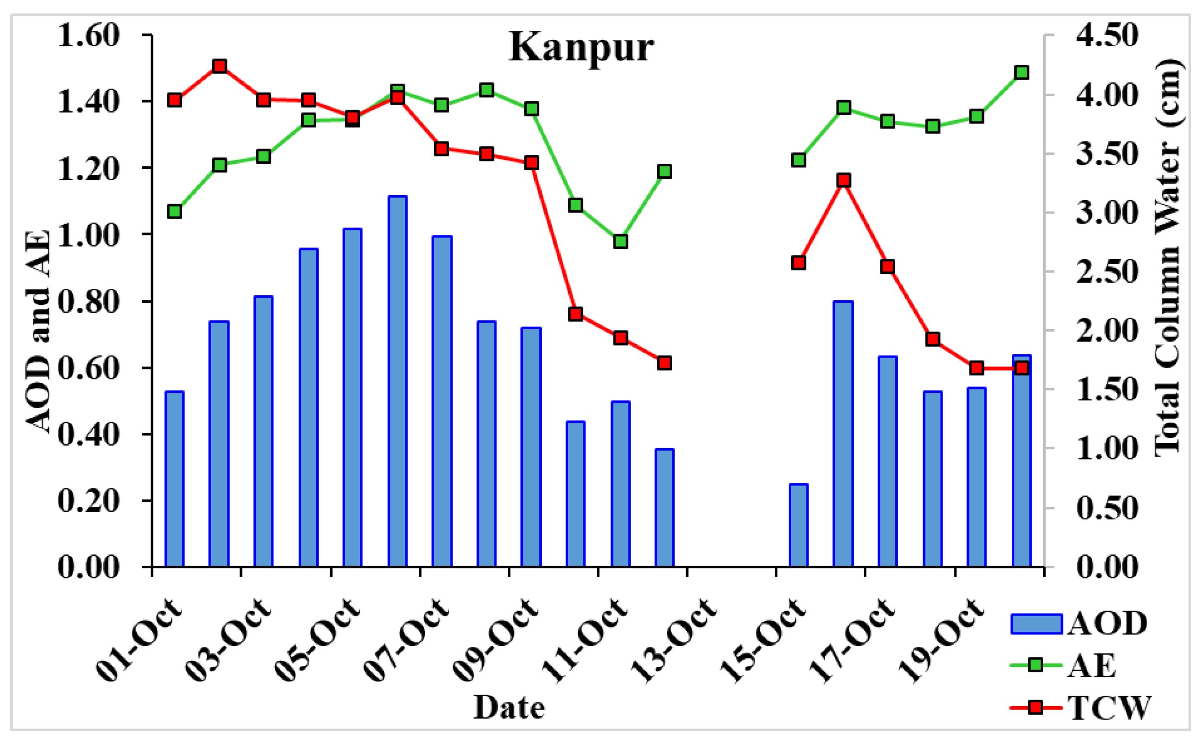
3.10. AOD, Angstrom Exponent (AE), and Total Column Water (TCW)
3.11. Single Scattering Albedo (SSA)
4. Conclusions
Author Contributions
Funding
Acknowledgments
Conflicts of Interest
References
- Singh, R.P. Early warning of natural hazards using satellite remote sensing. Curr. Sci. 2003, 89, 592–593. [Google Scholar]
- Cervone, G.; Singh, R.P.; Kafatos, M.; Yu, C. Wavelet maxima curves of surface latent heat flux anomalies associated with Indian earthquakes. Nat. Hazards Earth Syst. Sci. 2005, 5, 87–99. [Google Scholar] [CrossRef]
- Bhuiyan, C.; Singh, R.P.; Kogan, F.N. Monitoring drought dynamics in the Aravalli region (India) using different indices based on ground and remote sensing data. Int. J. Appl. Earth Obs. Geoinf. 2006, 8, 289–302. [Google Scholar] [CrossRef]
- Chauhan, A.; Zheng, S.; Xu, M.; Cao, C.; Singh, R.P. Characteristic changes in aerosol and meteorological parameters associated with dust event of 9 March 2013 Model. Earth Syst. Environ. 2016, 2, 1–10. [Google Scholar] [CrossRef]
- Behere, P.B.; Bhise, M.C. Farmers’ Suicide: Across Culture. Indian J. Psychiatry 2009, 51, 242–243. [Google Scholar] [CrossRef] [PubMed]
- Chow, E.C.H.; Li, R.C.V.; Zhou, W. Influence of Tropical Cyclones on Hong Kong Air Quality. Adv. Atmos. Sci. 2018, 35, 1177–1188. [Google Scholar] [CrossRef]
- Sarkar, S.; Singh, R.P.; Chauhan, A. Crop residue burning in northern India: Increasing threat to Greater India. J. Geophys. Res. Atmos. 2018, 123, 6920–6934. [Google Scholar] [CrossRef]
- Singh, R.P.; Cervone, G.; Kafatos, M.; Prasad, A.K.; Sahoo, A.K.; Sun, D.; Tang, D.L.; Yang, R. Multi-sensor studies of the Sumatra earthquake and tsunami of 26 December 2004. Int. J. Remote Sens. 2007, 28, 13–14. [Google Scholar] [CrossRef]
- Tang, D.L.; Satyanarayana, B.; Zhao, H.; Singh, R.P. A Preliminary Analysis of the Influence of Sumatran Tsunami on Indian Ocean CHL-A and SST. Adv. Geosci. 2006, 5, 15–20. [Google Scholar]
- Tang, D.; Zhao, H.; Satyanarayana, B.; Zheng, G.; Singh, R.P.; Lv, J.; Yan, Z. Variations of chlorophyll-a in the northeastern Indian Ocean after the 2004 South Asian tsunami. Int. J. Remote Sens. 2009, 30, 4553–4565. [Google Scholar] [CrossRef]
- Beckerman, W. Economic growth and the environment: Whose growth? whose environment? World Dev. 1992, 20, 481–496. [Google Scholar] [CrossRef]
- Acaravci, A.; Ozturk, I. On the relationship between energy consumption, CO2 emissions and economic growth in Europe. Energy 2010, 35, 5412–5420. [Google Scholar] [CrossRef]
- Alam, A.; Azam, M.; Bin Abdullah, A.; Malik, I.A.; Khan, A.; Hamzah, T.A.A.T.; Khan, M.M.; Zahoor, H.; Zaman, K. Environmental quality indicators and financial development in Malaysia: Unity in diversity. Environ. Sci. Pollut Res. 2014, 22, 8392–8404. [Google Scholar] [CrossRef] [PubMed]
- Boutabba, M.A. The impact of financial development, income, energy and trade on carbon emissions: Evidence from the Indian economy. Econ. Model. 2014, 40, 33–41. [Google Scholar] [CrossRef]
- Schandl, H.; Hatfield-Dodds, S.; Wiedmann, T.; Geschke, A.; Cai, Y.; West, J.; Newth, D.; Baynes, T.; Lenzen, M.; Owen, A. Decoupling global environmental pressure and economic growth: Scenarios for energy use, materials use and carbon emissions. J. Clean. Prod. 2016, 132, 45–56. [Google Scholar] [CrossRef]
- Ahmed, K.; Shahbaz, M.; Qasim, A.; Long, W. The linkages between deforestation, energy and growth for environmental degradation in Pakistan. Ecol. Indic. 2015, 49, 95–103. [Google Scholar] [CrossRef]
- Babu, T.S.A.; Kaechele, H. Dichotomy in carbon dioxide emissions: The case of India. Clim. Dev. 2015, 7, 165–174. [Google Scholar] [CrossRef]
- Rani, N.N.V.S.; Satyanarayana, A.N.V.; Bhaskaran, P.K. Coastal vulnerability assessment studies over India: A review. Nat. Hazards 2015, 77, 405–428. [Google Scholar] [CrossRef]
- Ohlan, R. The impact of population density, energy consumption, economic growth and trade openness on CO2 emissions in India. Nat. Hazards 2015, 79, 1409–1428. [Google Scholar] [CrossRef]
- Sarkar, S.; Singh, R.P.; Chauhan, A. Anomalous changes in meteorological parameters along the track of 2017 Hurricane Harvey. Remote Sens. Lett. 2018, 9, 487–496. [Google Scholar] [CrossRef]
- De, U.S.; Dube, R.K.; Rao, G.S.P. Extreme weather events over India in last 100 years. J. Indian Geophys. Union 2005, 9, 173–187. [Google Scholar]
- Prasad, A.K.; Singh, R.P. Changes in aerosol parameters during major dust storm events (2001–2005) over the Indo-Gangetic Plains using AERONET and MODIS data. J. Geophys Res. 2007, 112, D09208. [Google Scholar] [CrossRef]
- Sarkar, S.; Singh, R.P. June 19 2015 Rainfall Event Over Mumbai: Some Observational Analysis. J. Indian Soc Remote Sens. 2017, 45, 185. [Google Scholar] [CrossRef]
- Thomas, J.; Prasannakumar, V. Temporal analysis of rainfall (1871–2012) and drought characteristics over a tropical monsoon-dominated State (Kerala) of India. J. Hydrol. 2016, 534, 266–280. [Google Scholar] [CrossRef]
- Disaster Management of India: A status Report, Natural Disaster Management Division, Ministry of Home Affairs, Government of India, New Delhi. 2004. Available online: http://www.tezu.ernet.in/cdm/cdm_linkfile/link/study_material/indiastastsreport.pdf (accessed on 11 July 2018).
- Dey, S.; Tripathi, S.N.; Singh, R.P.; Holben, B.N. Influence of dust storms on the aerosol optical properties over the Indo-Gangetic basin. J. Geophys. Res. 2004, 109, D20211. [Google Scholar] [CrossRef]
- Gautam, R.; Hsu, N.C.; Tsay, S.C.; Lau, K.M.; Holben, B.; Bell, S.; Smirnov, A.; Li, C.; Hansell, R.; Ji, Q.; et al. Accumulation of aerosols over the Indo-Gangetic plains and southern slopes of the Himalayas: Distribution, properties and radiative effects during the 2009 pre-monsoon season. Atmos. Chem. Phys. 2011, 11, 12841–12863. [Google Scholar] [CrossRef]
- Gautam, R.; Hsu, C.N.; Eck, T.F.; Holben, B.N.; Janjai, S.; Jantarach, T.; Tsay, S.-C.; Lau, W.K. Characterization of aerosols over the Indochina peninsula from satellite-surface observations during biomass burning pre-monsoon season. Atmos. Environ. 2013, 78, 51–59. [Google Scholar] [CrossRef]
- Kaskaoutis, D.G.; Kumar, S.; Sharma, D.; Singh, R.P.; Kharol, S.K.; Sharma, M.; Singh, A.K.; Singh, S.; Singh, A.; Singh, D. Effects of crop residue burning on aerosol properties, plume characteristics, and long-range transport over northern India. J. Geophys. Res. Atmos. 2014, 119, 5424–5444. [Google Scholar] [CrossRef]
- Singh, R.P.; Kaskaoutis, D.G. Crop residue burning: A threat to South Asian air quality. Eos Trans. Am. Geophys. Union 2014, 95, 333–334. [Google Scholar] [CrossRef]
- Chauhan, A.; Singh, R.P. Poor air quality and dense haze/smog during 2016 in the indo-gangetic plains associated with the CRB and Diwali festival. In Proceedings of the IEEE International Geoscience and Remote Sensing Symposium (IGARSS), Fort Worth, TX, USA, 23–28 July 2017. [Google Scholar]
- Arif, M.; Kumar, R.; Kumar, R.; Zusman, E.; Singh, R.P.; Gupta, A. Assessment of indoor & outdoor black carbon emissions rural areas of Indo-Gangetic plain: Seasonal characteristics, source apportionment and radiative forcing. Atmos. Environ. 2018, in press. [Google Scholar]
- Nicholls, R.J. Coastal megacities and climate change. Geo J. 1995, 37, 369–379. [Google Scholar] [CrossRef]
- Pendleton, E.A.; Thieler, E.R.; Jeffress, S.W. Coastal Vulnerability Assessment of Golden Gate National Recreation Area to Sea-Level Rise; USGS Open-File Report; USGS: Reston, VI, USA, 2005; p. 1058. [Google Scholar]
- Knutson, T.R.; McBride, J.L.; Chan, J.; Emanuel, K.; Holland, G.; Landsea, C.; Held, I.; Kossin, J.P.; Srivastava, A.K.; Sugi, M. Tropical cyclones and climate change. Nat. Geosci. 2010, 3, 157–163. [Google Scholar] [CrossRef]
- Kafatos, M.; Sun, D.; Gautam, R.; Boybeyi, Z.; Yang, R.; Cervone, G. Role of anomalous warm gulf waters in the intensification of Hurricane Katrina. Geophys. Res. Lett. 2006, 33, L17802. [Google Scholar] [CrossRef]
- Gautam, R.; Cervone, G.; Singh, R.P.; Kafatos, M. Characteristics of meteorological parameters associated with Hurricane Isabel. Geophys. Res. Lett. 2005, 32, L04801. [Google Scholar] [CrossRef]
- Hoarau, K.; Bernard, J.; Chalonge, L. Intense tropical cyclone activities in the northern Indian Ocean. Int. J. Climatol. 2012, 32, 1935–1945. [Google Scholar] [CrossRef]
- Kundu, S.N.; Sahoo, A.K.; Mohapatra, S.; Singh, R.P. Change analysis using IRS-P4 OCM data after the Orissa super cyclone. Int. J. Remote Sens. 2001, 22, 1383–1389. [Google Scholar] [CrossRef]
- Murali, R.M.; Ankita, M.; Vethamony, P. A new insight to vulnerability of Central Odisha coast, India using analytical hierarchical process (AHP) based approach. J. Coast. Conserv. 2017, 22, 799–819. [Google Scholar]
- Shay, L.K.; Goni, G.J.; Black, P.G. Effects of a warm oceanic feature on Hurricane Opal. Mon. Weather Rev. 2000, 128, 1366–1383. [Google Scholar] [CrossRef]
- Gautam, R.; Singh, R.P.; Kafatos, M. Changes in ocean properties associated with Hurricane Isabel. Int. J. Remote Sens. 2005, 26, 643–649. [Google Scholar] [CrossRef]
- Pathakoti, M.; Sujatha, P.; Karri, S.R.; Sai Krishn, S.V.S.; Rao, P.V.N.; Dutt, C.B.S.; Dadhwal, V.K. Evidence of stratosphere-troposphere exchange during severe cyclones: A case study over Bay of Bengal, India. Geomatics. Nat. Hazards Risk 2016, 7, 1816–1823. [Google Scholar] [CrossRef]
- Cyclone Hudhud: Strategies and Lessons for Preparing Better & Strengthening Risk Resilience in Coastal Regions of India, National Disaster Management Authority of India, August 2015. Available online: https://ndma.gov.in/images/pdf/Hudhud-lessons.pdf (accessed on 11 July 2018).
- Chejarla, V.R.; Mandla, V.R.; Palanisamy, G.; Choudhary, M. Estimation of damage to agriculture biomass due to Hudhud cyclone and carbon stock assessment in cyclone affected areas using Landsat-8. Geocarto Int. 2017, 32, 589–602. [Google Scholar] [CrossRef]
- Reynolds, R.W.; Smith, T.M.; Chunying, L.D.B.; Chelton, K.S.C.; Schlax, M.G. Daily High-Resolution-Blended Analyses for Sea Surface Temperature. J. Clim. 2007, 20, 5473–5496. [Google Scholar] [CrossRef]
- Holben, B.N.; Eck, T.F.; Slutsker, I.; Tanre, D.; Buis, J.P.; Setzer, A.; Vermote, E.; Reagan, J.A.; Kaufman, Y.J.; Nakajima, T.; et al. AERONET—A federated instrument network and data archive for aerosol characterization. Remote Sens. Environ. 1998, 66, 1–16. [Google Scholar] [CrossRef]
- Dubovik, O.; King, M.D. A flexible inversion algorithm for retrieval of aerosol optical properties from Sun and sky radiance measurements. J. Geophys. Res. 2000, 105, 20673–20696. [Google Scholar] [CrossRef]
- Dubovik, O.; Smirnov, A.; Holben, B.N.; King, M.D.; Kaufman, Y.J.; Eck, T.F.; Slutsker, I. Accuracy assessments of aerosol optical properties retrieved from Aerosol Robotic federated instrument network and data archive for aerosol characterization. J. Geophys. Res. 2000, 105, 9791–9806. [Google Scholar] [CrossRef]
- Evan, A.T.; Kossin, J.P.; Chung, C. ‘Eddy’, Ramanathan, V. Arabian Sea tropical cyclones intensified by emissions of black carbon and other aerosols. Nature 2011, 479, 94–97. [Google Scholar] [CrossRef]


| Box | West | South | East | North |
|---|---|---|---|---|
| Box 1 | 81.22 | 17.69 | 83.22 | 19.69 |
| Box 2 | 79.54 | 19.84 | 81.54 | 21.84 |
| Box 3 | 79.33 | 22.67 | 81.33 | 24.67 |
| Box 4 | 79.23 | 25.51 | 81.23 | 27.51 |
| Box 5 | 83.48 | 15.69 | 85.48 | 17.69 |
| Location | (Center Latitude) North | (Center Longitude) East |
|---|---|---|
| Location 1 | 17.50 | 82.50 |
| Location 2 | 20.00 | 80.00 |
| Location 3 | 25.00 | 80.00 |
| Location 4 | 27.50 | 80.00 |
| S.No. | Parameters | Source |
|---|---|---|
| 1 | Surface Temperature | AIRS/Giovanni |
| 2 | SST Anomaly | NOAA NCDC |
| 3 | Relative Humidity | NCEP NCAR |
| 4 | Omega | NCEP NCAR |
| 5 | Wind Speed and Direction | NCEP NCAR |
| 6 | Surface Latent Heat Flux | NCEP NCAR |
| 7 | Tropopause Pressure | AIRS/Giovanni |
| 8 | Total Column Ozone | AIRS/Giovanni |
| 9 | CO VMR | AIRS/Giovanni |
| 10 | H2O MMR | AIRS/Giovanni |
| 11 | Aerosol Optical Depth (AOD) | MODIS and AERONET |
| 12 | Angstrom Exponent (AE) | MODIS and AERONET |
| 13 | Total Column Water (TCW) | AERONET |
| 14 | Rainfall | TRMM/Giovanni |
© 2018 by the authors. Licensee MDPI, Basel, Switzerland. This article is an open access article distributed under the terms and conditions of the Creative Commons Attribution (CC BY) license (http://creativecommons.org/licenses/by/4.0/).
Share and Cite
Chauhan, A.; Kumar, R.; Singh, R.P. Coupling between Land–Ocean–Atmosphere and Pronounced Changes in Atmospheric/Meteorological Parameters Associated with the Hudhud Cyclone of October 2014. Int. J. Environ. Res. Public Health 2018, 15, 2759. https://doi.org/10.3390/ijerph15122759
Chauhan A, Kumar R, Singh RP. Coupling between Land–Ocean–Atmosphere and Pronounced Changes in Atmospheric/Meteorological Parameters Associated with the Hudhud Cyclone of October 2014. International Journal of Environmental Research and Public Health. 2018; 15(12):2759. https://doi.org/10.3390/ijerph15122759
Chicago/Turabian StyleChauhan, Akshansha, Rajesh Kumar, and Ramesh P. Singh. 2018. "Coupling between Land–Ocean–Atmosphere and Pronounced Changes in Atmospheric/Meteorological Parameters Associated with the Hudhud Cyclone of October 2014" International Journal of Environmental Research and Public Health 15, no. 12: 2759. https://doi.org/10.3390/ijerph15122759
APA StyleChauhan, A., Kumar, R., & Singh, R. P. (2018). Coupling between Land–Ocean–Atmosphere and Pronounced Changes in Atmospheric/Meteorological Parameters Associated with the Hudhud Cyclone of October 2014. International Journal of Environmental Research and Public Health, 15(12), 2759. https://doi.org/10.3390/ijerph15122759