Algal Bloom Prediction Using Extreme Learning Machine Models at Artificial Weirs in the Nakdong River, Korea


Abstract
1. Introduction
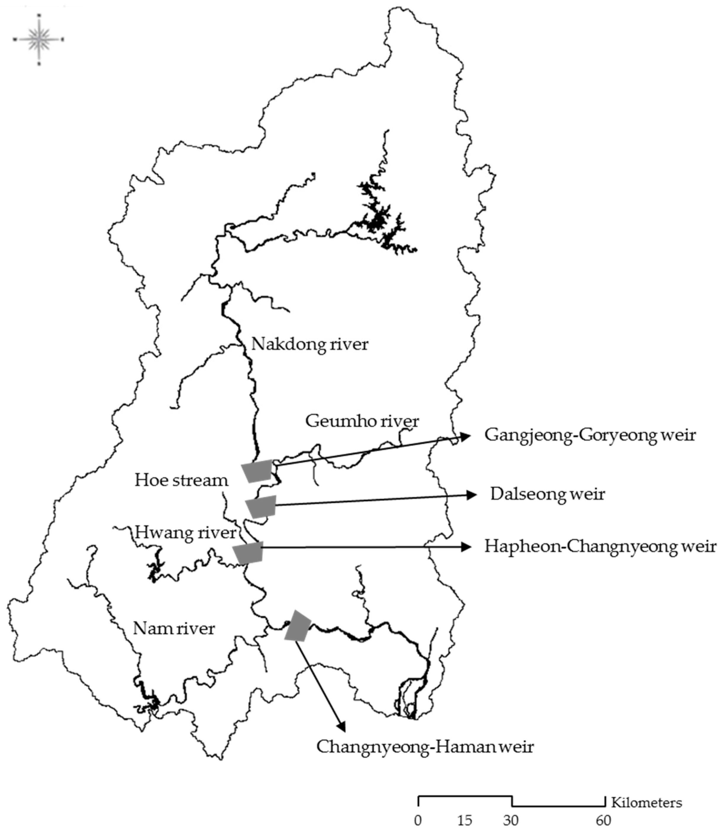
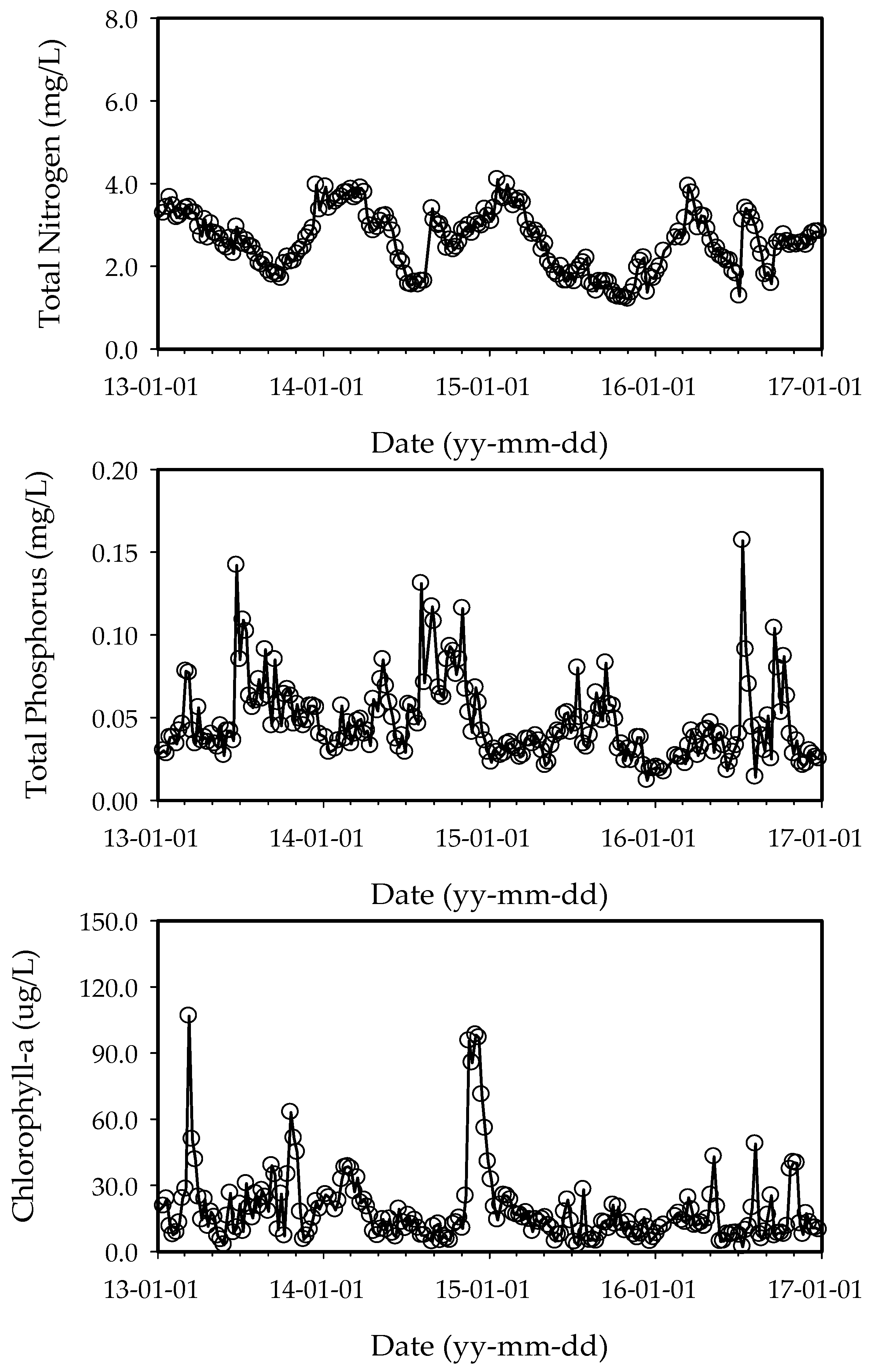
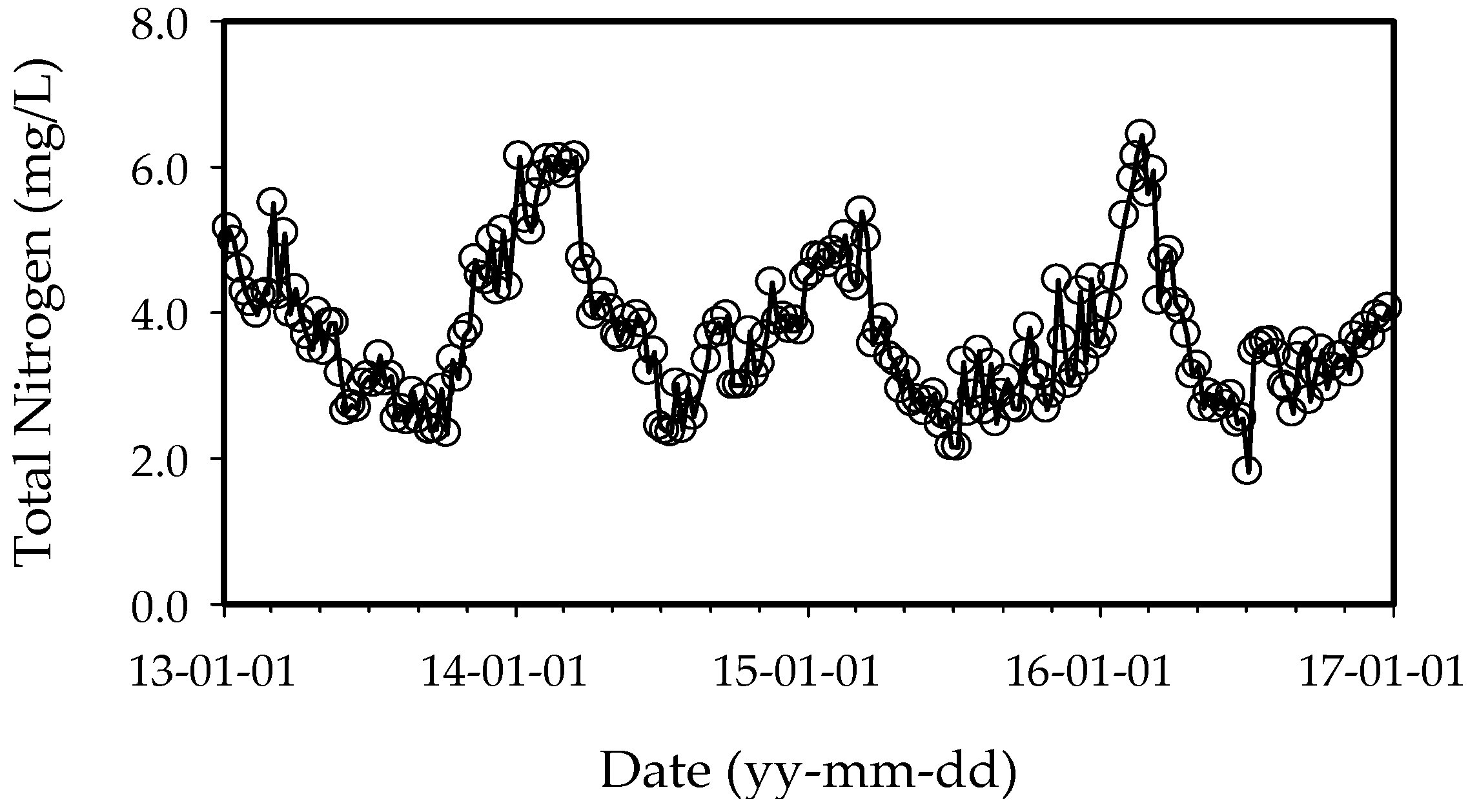
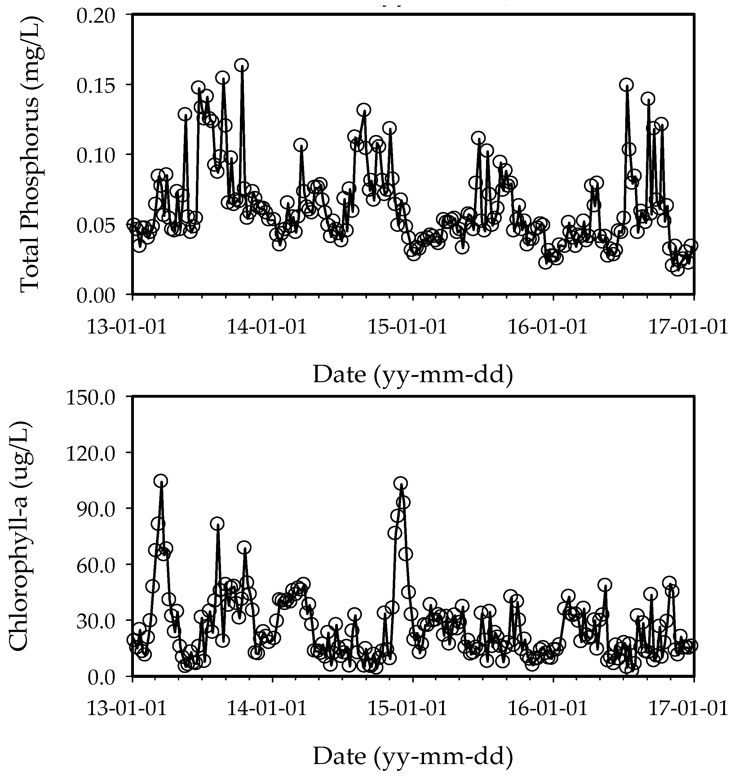
2. Study Area
3. Extreme Learning Machine
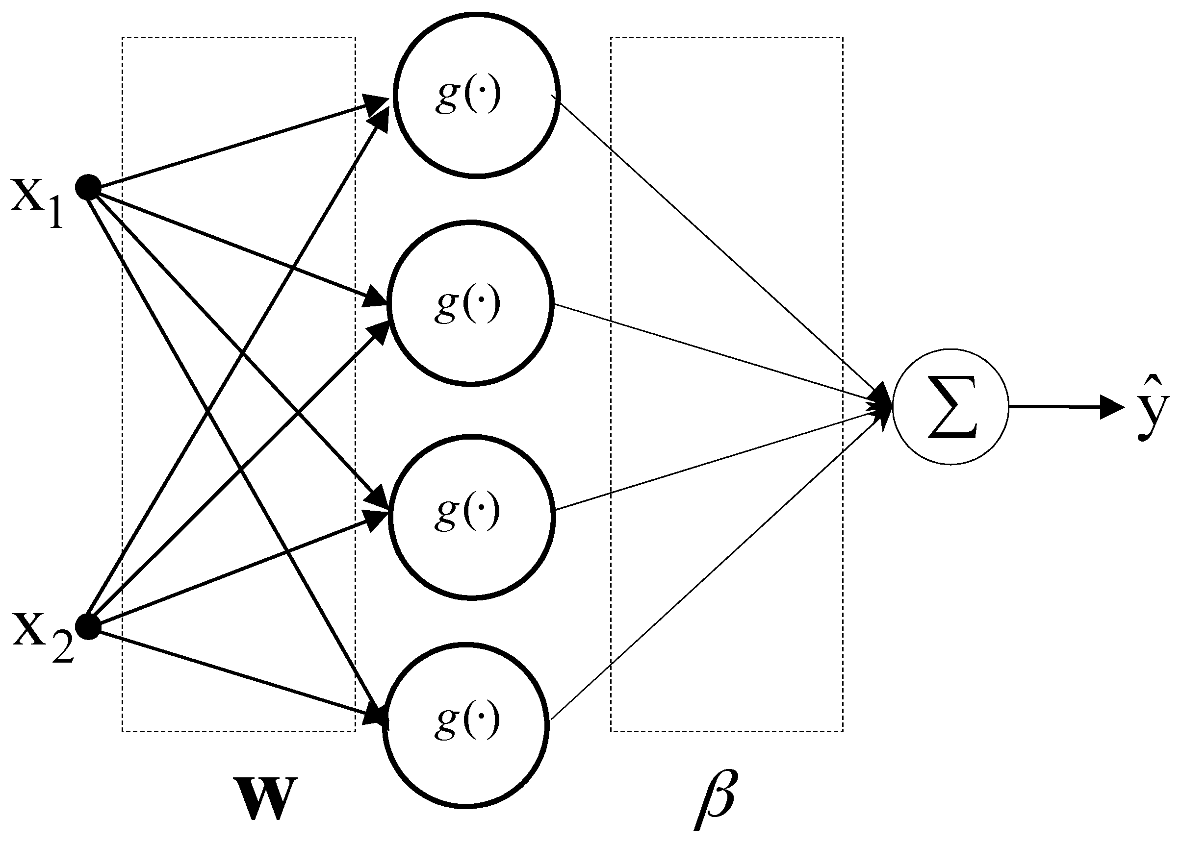
3.1. Architecture and Learning Method for ELM
- (Step 1) Randomly assign hidden node parameters
- (Step 2) Calculate the hidden layer output matrix
- (Step 3) Calculate the output weights β using a least squares estimate (LSE):where is the Moore-Penrose generalized inverse of matrix H. When is nonsingular, is the pseudo-inverse of H. This is a standard LSE problem, and the best solution for β is expressed as follows [16]:
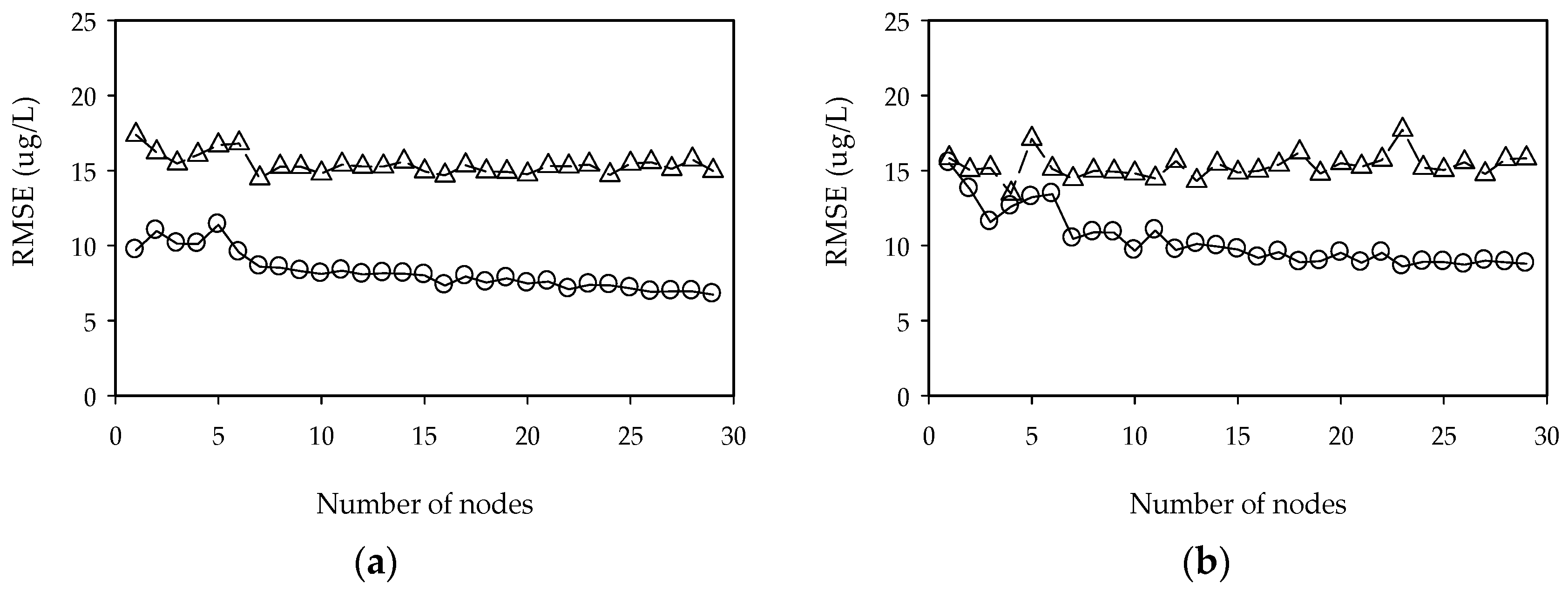
3.2. Model Application
4. Results and Discussion
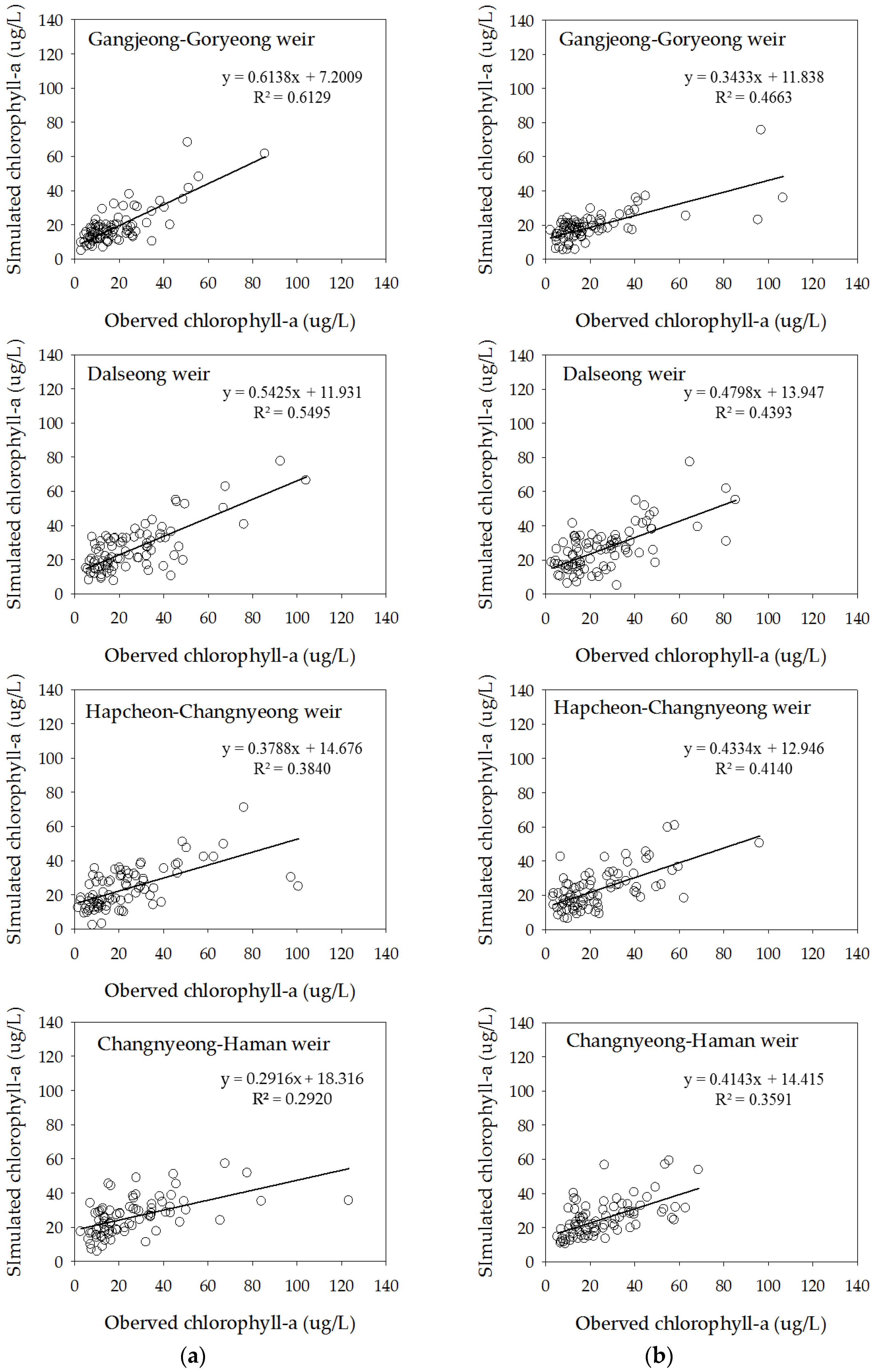
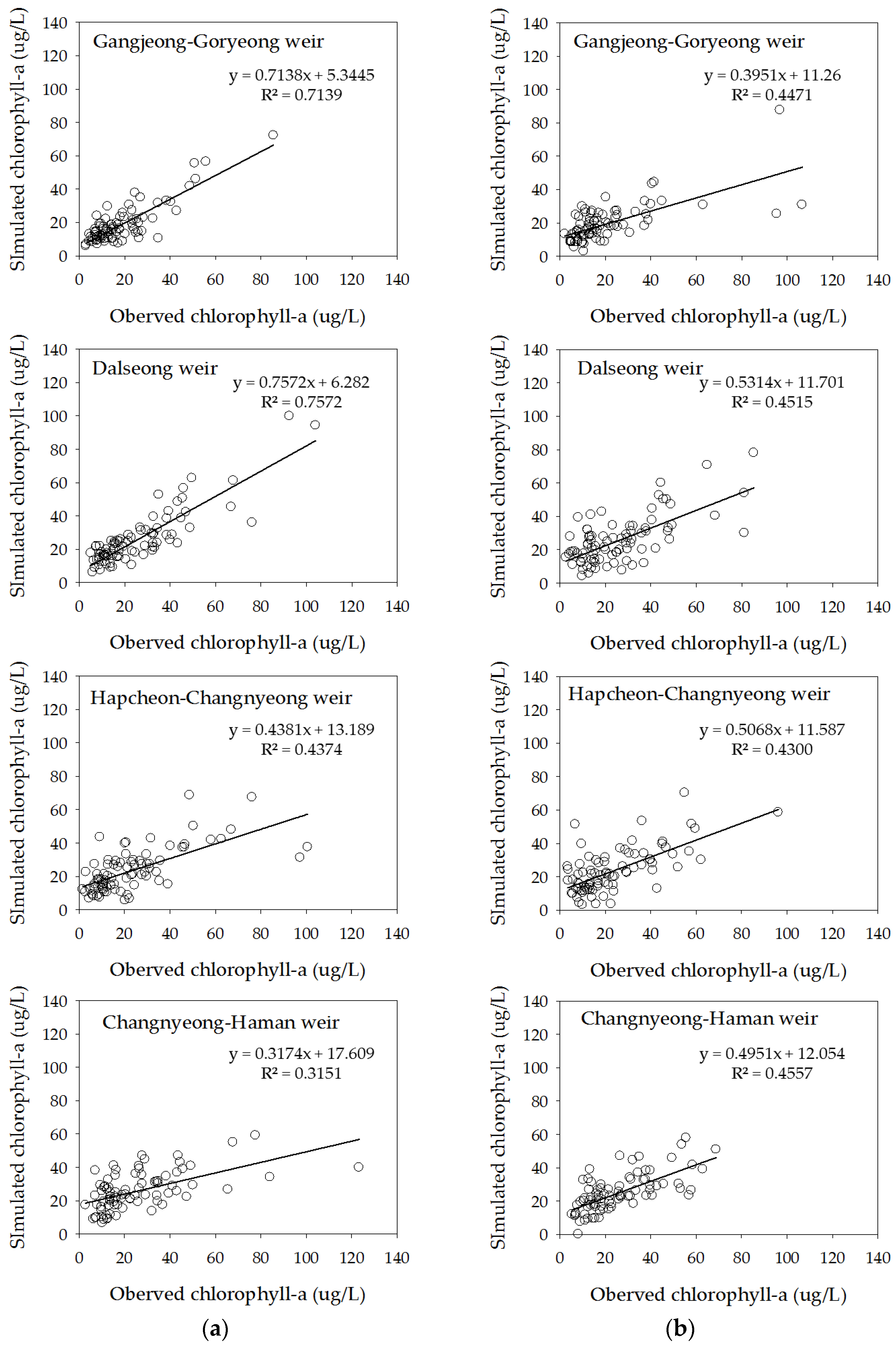
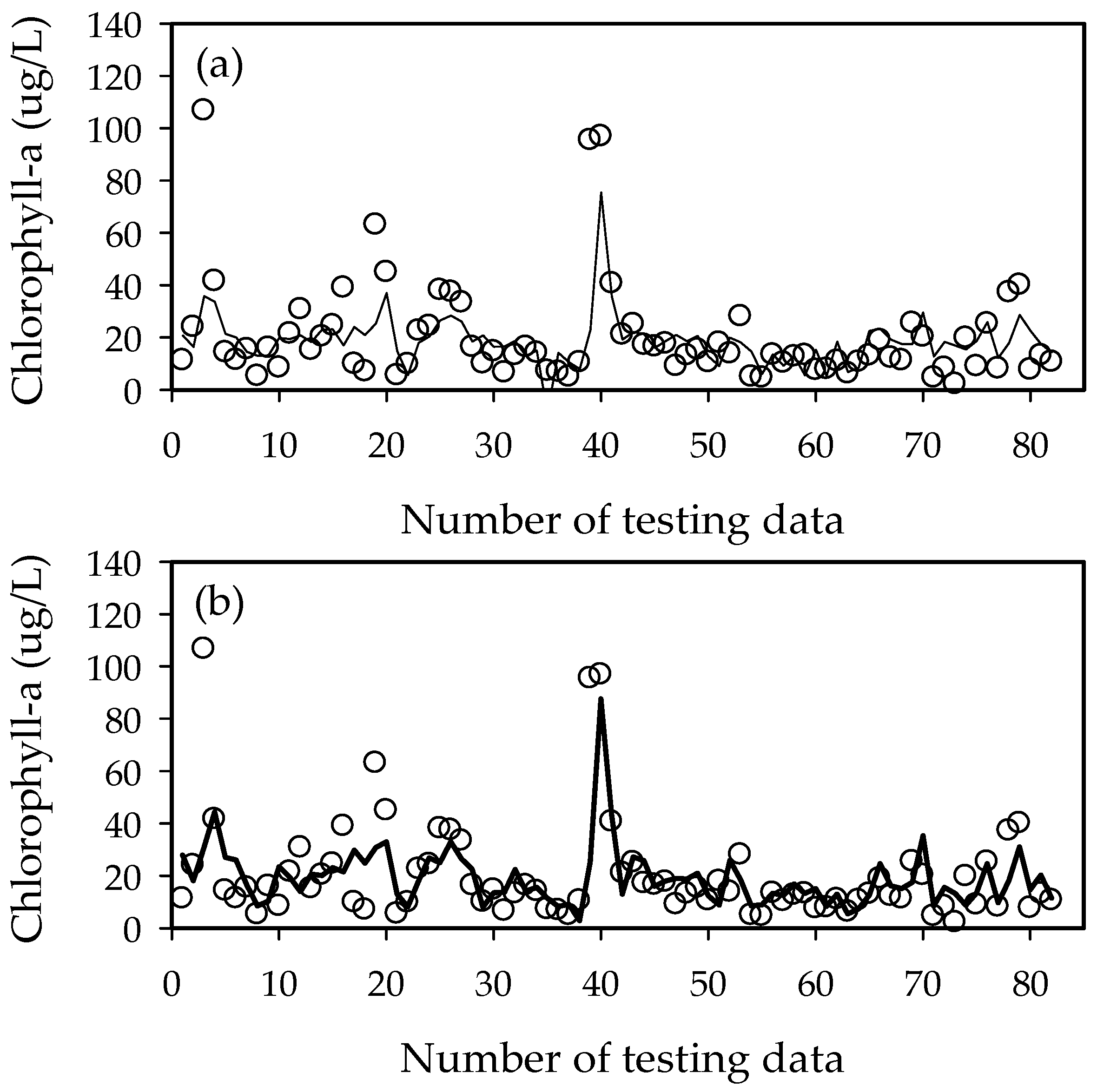
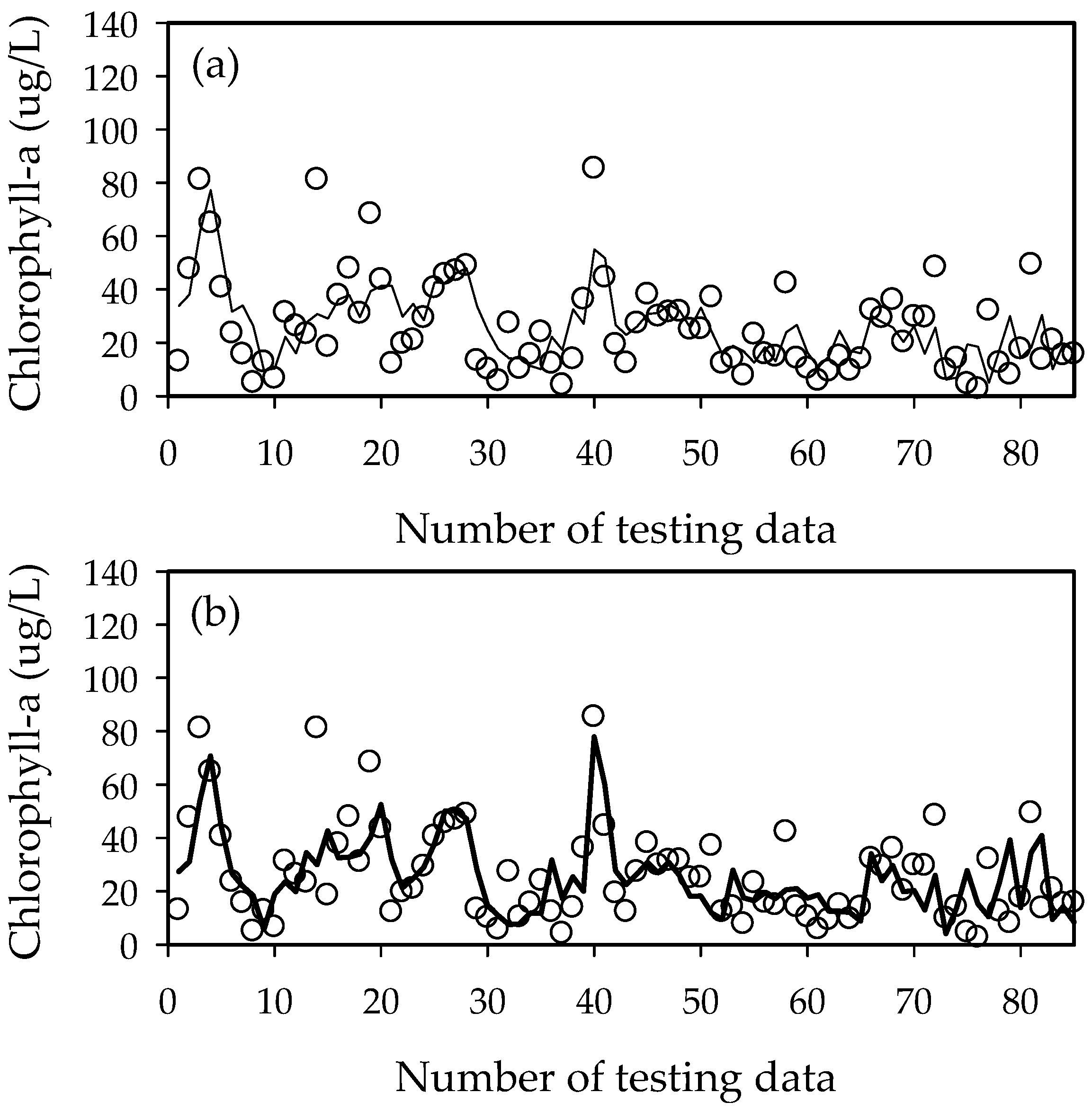
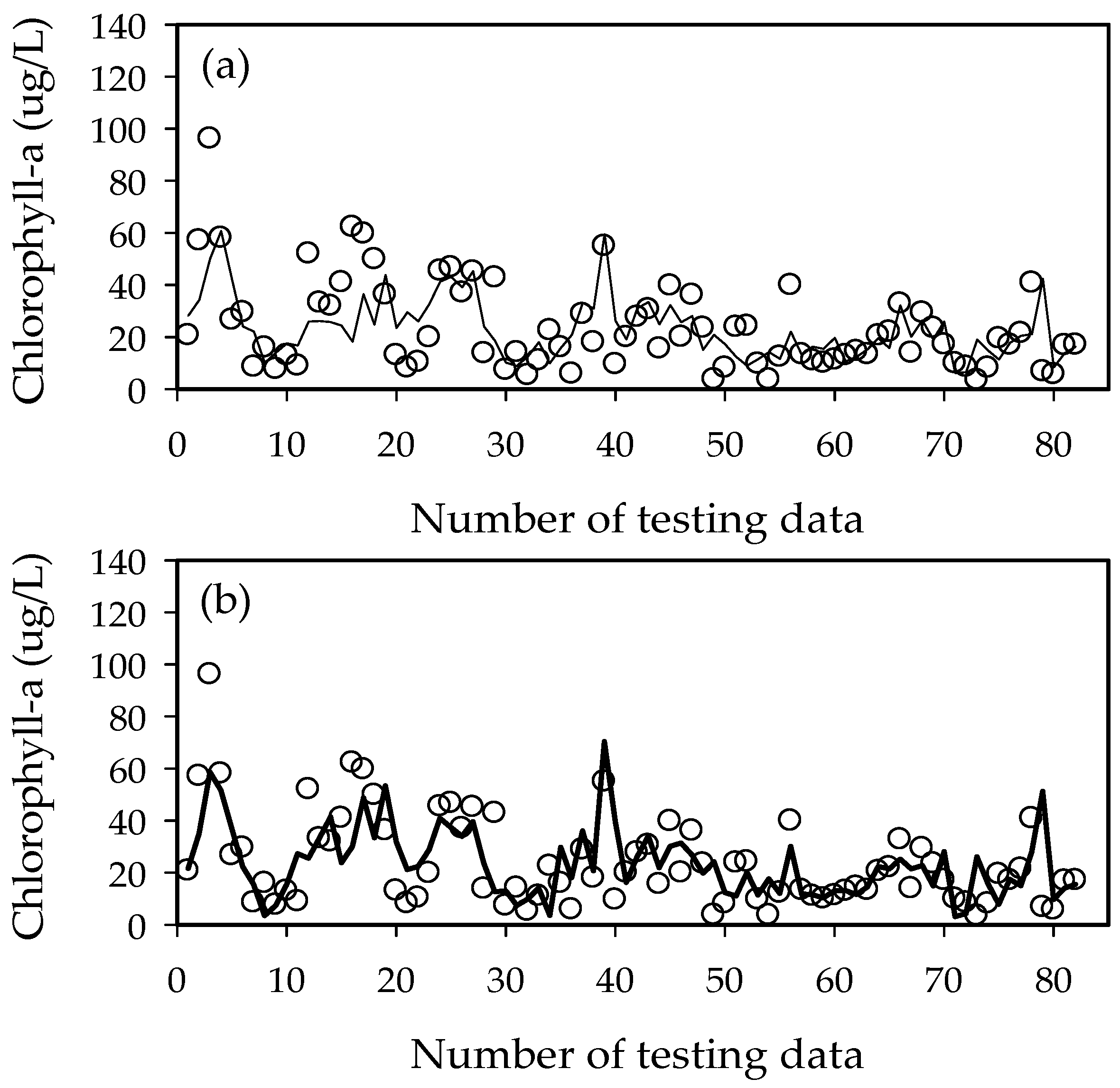
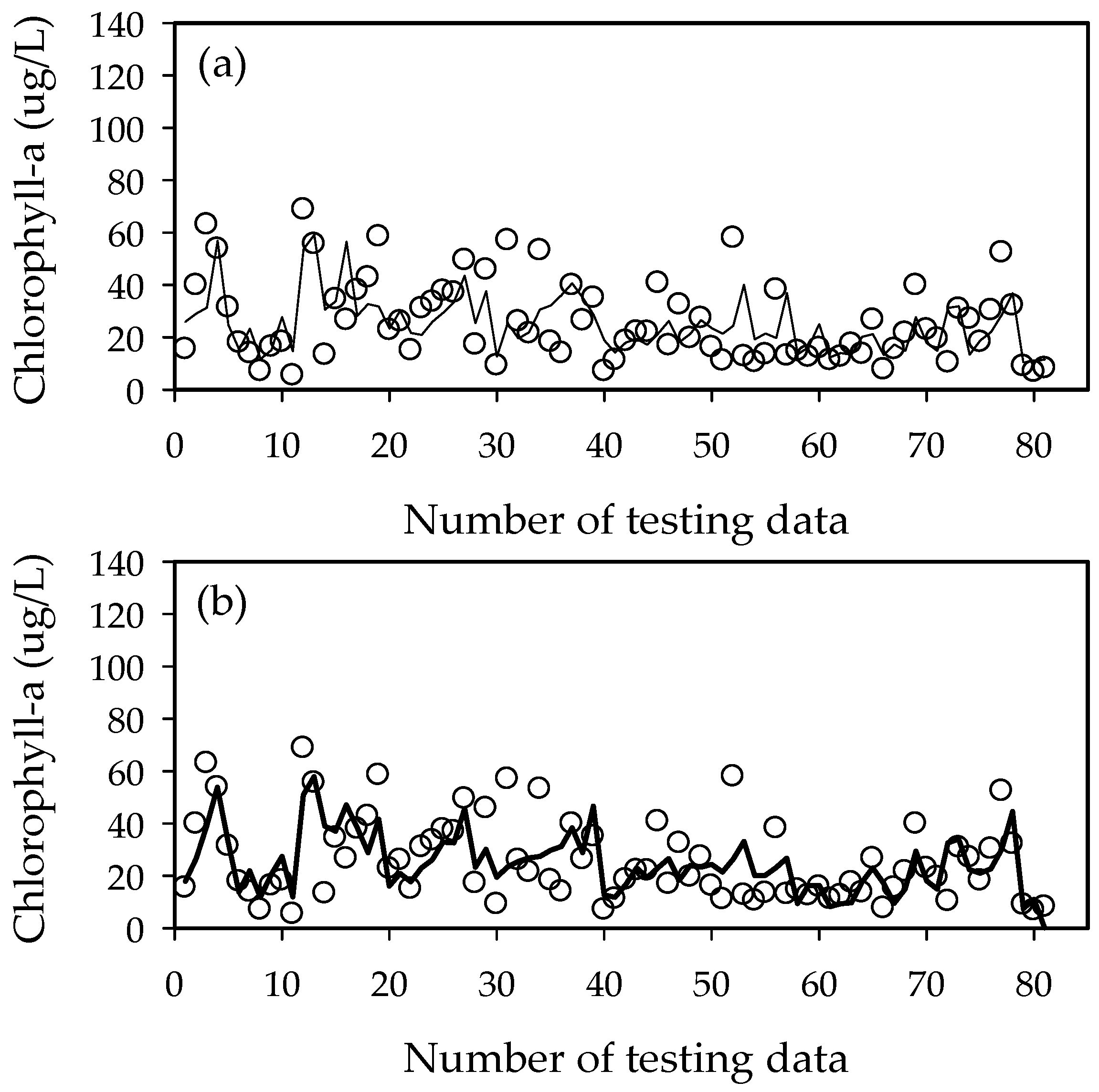
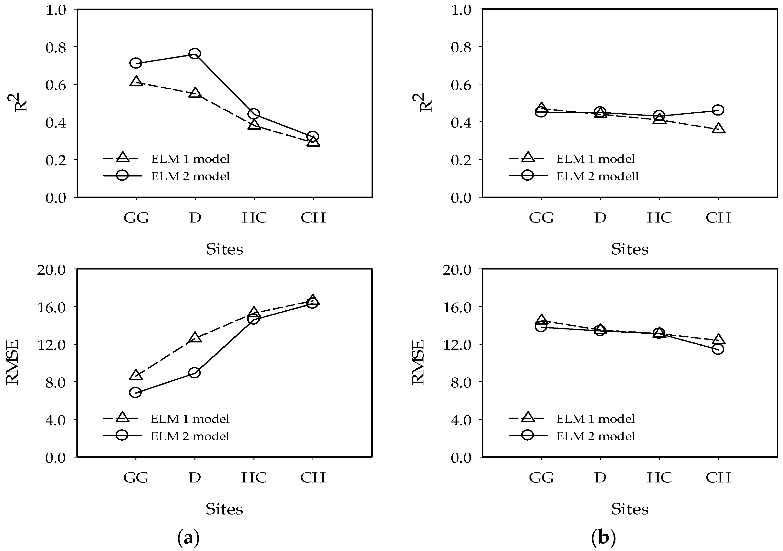
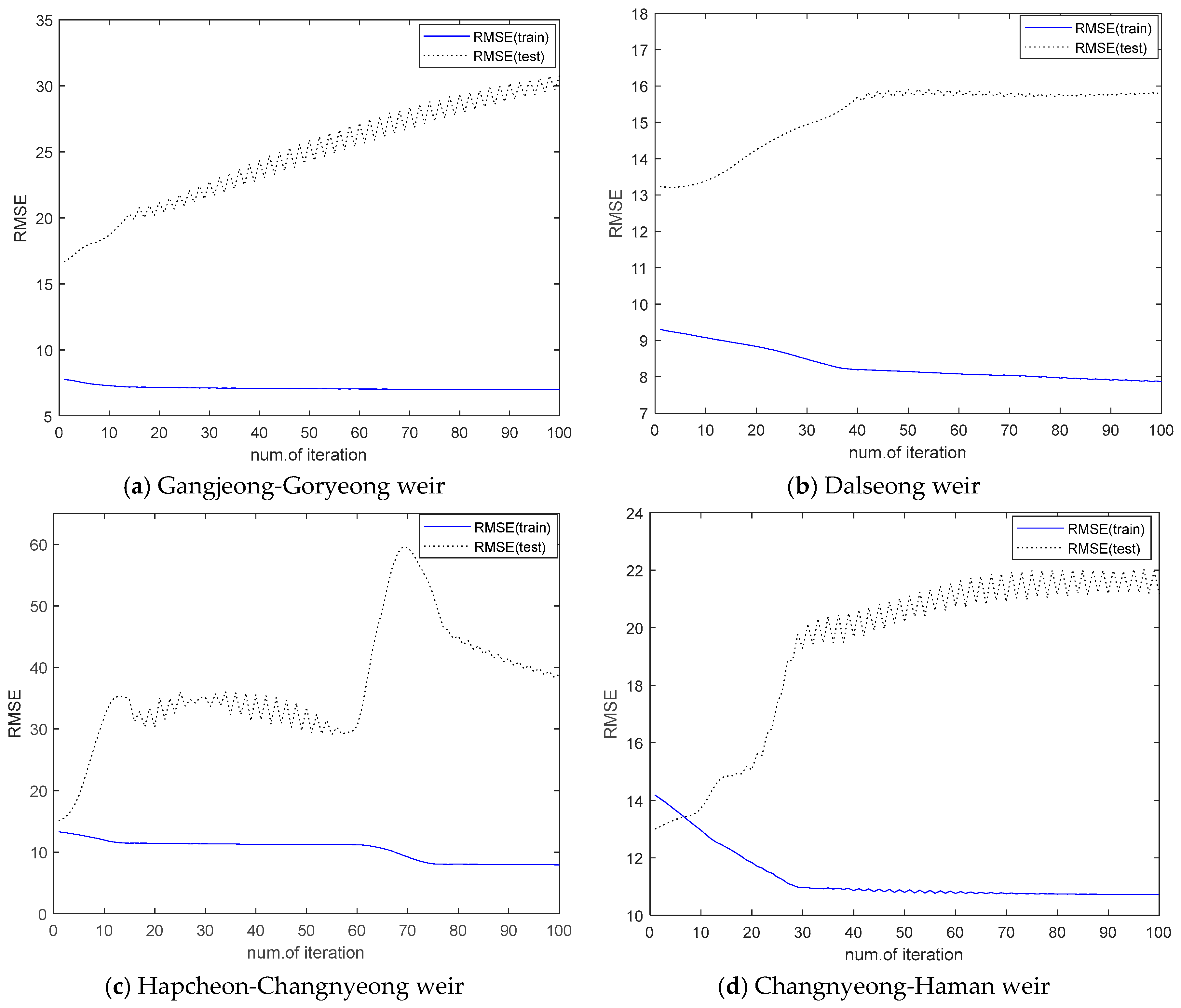
4.1. Experimental Results
4.2. ELM Performance Discussion
- -
- ELM consists of a simple tuning-free three-step algorithm.
- -
- The learning speed of ELM is extremely fast.
- -
- The hidden node parameters are independent of training data. Although hidden nodes are important, they need not be tuned.
- -
- ELM could generate the hidden node parameters before using the training data.
- -
- ELM can be effectively applied to most real-world problems such as compression, feature learning, clustering, regression and classification.
5. Conclusions
Author Contributions
Funding
Acknowledgments
Conflicts of Interest
References
- Anderson, D.M.; Cembella, A.D.; Hallegraeff, G.M. Progress in understanding harmful algal blooms: Paradigm shifts and new technologies for research, monitoring, and management. Ann. Rev. Mar. Sci. 2012, 4, 143–176. [Google Scholar] [CrossRef] [PubMed]
- Zhang, F.; Wang, Y.; Cao, M.; Sun, X.; Du, Z.; Liu, R.; Ye, X. Deep-Learning-Based Approach for Prediction of Algal Blooms. Sustainability 2016, 8, 1060. [Google Scholar] [CrossRef]
- Tian, W.; Liao, Z.; Zhang, J. An Optimization of artificial neural network model for predicting chlorophyll hynamics. Ecol. Model. 2017, 364, 42–52. [Google Scholar] [CrossRef]
- Ye, L.; Cai, Q.; Zhang, M.; Tan, L. Real-time observation, early warning and forecasting phytoplankton blooms by integrating in situ automated online sondes and hybrid evolutionary algorithm. Ecol. Inform. 2014, 22, 44–51. [Google Scholar] [CrossRef]
- Conley, D.J.; Paeral, H.W.; Howarth, R.W.; Boesch, D.F.; Seitzinger, S.P.; Haven, K.E.; Lancelot, C.; Liken, G.E. Controlling Eutrophication: Nitrogen and Phosphorus. Science 2009, 323, 1014–1015. [Google Scholar] [CrossRef] [PubMed]
- Recknagel, F.; French, M.; Harkonen, P.; Yabunaka, K.I. Artifitial neural network approach for modelling and prediction of algal blooms. Ecol. Model. 1997, 96, 11–28. [Google Scholar] [CrossRef]
- Zhang, X.; Recknagel, F.; Chen, Q.; Cao, H.; Li, R. Spatially-explicit modelling and forecasting of cyanobacteria growth in Lake Taihu by evolutionary computation. Ecol. Model. 2014, 306, 216–225. [Google Scholar] [CrossRef]
- Xie, Z.; Lou, I.; Ung, W.K.; Mok, K.M. Freshwater algal bloom prediction by Support vector machine in Macau Storage Reservoirs. Math. Probl. Eng. 2012, 27, 1–12. [Google Scholar] [CrossRef]
- Loi, I.; Xie, Z.; Ung, W.K. Freshwater algal bloom prediction by extreme learning machine in Macau Storage Reservoirs. Neural Comput. Appl. 2016, 27, 19–26. [Google Scholar] [CrossRef]
- Rogers, L.L.; Dowla, F.U. Optimization of groundwater remediation using artificial neural network with parallel solute transport modeling. Water Resour. Res. 1994, 30, 457. [Google Scholar] [CrossRef]
- Wong, K.I.; Wong, P.K.; Cheung, C.S.; Vong, C.M. Modeling and optimization of biodiesel engine performance using advanced machine learning methods. Energy 2013, 55, 519–529. [Google Scholar] [CrossRef]
- Deng, W.Y.; Zheng, Q.H.; Chen, L.; Xu, X.B. Power utility nontechnical loss analysis with extreme learning machine method. Chin. J. Comput. 2010, 33, 280–287. [Google Scholar] [CrossRef]
- Xu, Y.; Dai, Y.; Dong, Z.Y.; Zhang, R.; Meng, K. Extreme learning machine-based predictor for real-time frequency stability assessment of electric power systems. Neural Comput. Appl. 2013, 22, 501–508. [Google Scholar] [CrossRef]
- Sun, Z.I.; Ng, K.M.; Soszynska-Budny, J.; Habbullah, M.S. Application of the LP-ELM model on transportation system life-time optimization. IEEE Trans. Intell. Transp. Syst. 2011, 12, 1484–1494. [Google Scholar] [CrossRef]
- Vergara, G.; C’ozar, J.; Romero-Gonz’alez, C.; G’amez, J.A.; Soria-Olivas, E. Comparing ELM Against MLP for Electrical Power Prediction in Buildings. Bioinspired Comput. Artif. Syst. 2015, 409–418. [Google Scholar] [CrossRef]
- Yeom, C.U.; Kwak, K.C. Short-term electricity-load forecasting using a TSK-based extreme learning machine with knowledge representation. Energies 2017, 10, 1613. [Google Scholar] [CrossRef]
- Yadav, B.; Sudheer, C.; Shashi, M.; Adamowski, J. Discharge forecasting using an online sequential extreme learning machine (OS-ELM) model: A case study in Neckar River, Germany. Measurement 2016, 92, 433–445. [Google Scholar] [CrossRef]
- Yin, Z.; Peng, T.; Feng, Q.; Yang, L.; Deo, R.C.; Wen, X.; Si, J.; Xiao, S. Future Projection with an Extreme-Learning Machine and Support Vector Regression of Reference Evapotranspiration in a Mountainous Inland Watershed in North-West China. Water 2018, 9, 880. [Google Scholar] [CrossRef]
- Wang, L.; Wang, X.; Xu, Z.; Zhang, H.; Yao, J.; Jin, X.; Liu, C.; Shi, Y. Time-varying nonlinear modeling and analysis of algal bloom dynamics. Nonlinear Dyn. 2016, 84, 371–378. [Google Scholar] [CrossRef]
- Wang, X.; Yao, J.; Shi, Y.; Su, T.; Wang, L.; Xu, J. Research on hybrid mechanism modeling of algal bloom formation in urban lakes and reservoirs. Ecol. Model. 2016, 332, 67–73. [Google Scholar] [CrossRef]
- Wang, W.C.; Xu, D.M.; Chau, K.W.; Lei, G.J. Assessment of river water quality based on theory of variable fuzzy sets and fuzzy binary comparison method. Water Resour. Manag. 2014, 28, 4183–4200. [Google Scholar] [CrossRef]
- Olyaie, E.; Banejad, H.; Chau, K.W.; Melesse, A.M. A comparison of various artificial intelligence approaches performance for estimating suspended sediment load of river systems: A case study in United States. Environ. Monit. Assess. 2015, 187, 189. [Google Scholar] [CrossRef] [PubMed]
- Fotovatikhah, F.; Herrera, M.; Shamshirband, S.; Chau, K.W.; Ardabili, S.F.; Piran, M.J. Survey of computational intelligence as basis to big flood management: Challenges, research directions and future work. Eng. Appl. Comput. Fluid Mech. 2018, 12, 411–437. [Google Scholar] [CrossRef]
- Cha, Y.K.; Cho, K.H.; Lee, H.; Kang, T.K.; Kim, J.H. The relative importance of water temperature and residence time in predicting cyanobacteria abundance in regulated rivers. Water Res. 2017, 124, 11–19. [Google Scholar] [CrossRef] [PubMed]
- Paerl, H.W. Controlling cyanobacterial harmful blooms in freshwater ecosystems. Microb. Biotechnol. 2017, 10, 1106–1110. [Google Scholar] [CrossRef] [PubMed]
- U.S. Environmental Protection Agency. Water Quality Criteria Research of the U.S. Environmental Protection Agency: EPA-600/3-76-079. In Proceedings of the EPA Sponsored Symposium, Corvallis, OR, USA, 17–23 August 1975. [Google Scholar]
- Forsberg, C.; Ryding, S.O. Eutrophication parameters and trophic state indices in 30 Swedish waste-receiving lakes. Arch. Hydrobiol. 1980, 89, 189–207. [Google Scholar]
- Organisation for Economic Co-operation and Development (OECD). OECD Eutrophication Programme-Regional Project Alpine Lakes; Swiss Federal Board for Environmental Protection OECD: Bern, Switzerland, 1980. [Google Scholar]
- Huang, G.B.; Zhu, Q.Y.; Siew, C.K. Extreme learning machine; theory and applications. Neurocomputing 2006, 70, 489–501. [Google Scholar] [CrossRef]
- Huang, G.B.; Chen, L.; Siew, C.K. Universal approximation using incremental constructive feedforward networks with random hidden nodes. IEEE Trans. Neural Netw. 2006, 17, 879–892. [Google Scholar] [CrossRef] [PubMed]
- Akaike, H. Information theory and an extension of the maximum likelihood principle. In Proceedings of the Second International Symposium on Information Theory, Tsahkadsor, Armenia, 2–8 September 1971; Petrov, B.N., Csaki, F., Eds.; pp. 267–281. [Google Scholar]
- Yaseen, Z.M.; Ramal, M.M.; Diop, L.; Jaafar, O.; Demir, V.; Kisi, O. Hybrid Adaptive Neuro-Fuzzy Models for Water Quality Index Estimation. Water Resour. Manag. 2018, 32, 2227–2245. [Google Scholar] [CrossRef]
- Wang, W.C.; Chau, K.W.; Cheng, C.T.; Qiu, L. A comparison of performance of several artificial intelligence methods for forecasting monthly discharge time series. J. Hydrol. 2009, 374, 294–306. [Google Scholar] [CrossRef]
- Bruder, B.; Babbar-Sebens, M.; Tedesco, L.; Soyeux, E. Use of fuzzy logic models for prediction of taste and odor compounds in algal bloom-affected inland water bodies. Environ. Monit. Assess. 2014, 186, 1525–1545. [Google Scholar] [CrossRef] [PubMed]
- Gong, Y.; Zhang, Y.; Lan, S.; Wang, F. A Comparative Study of Artificial Neural Networks, Support Vector Machines and Adaptive Neuro Fuzzy Inference System for Forecasting Groundwater Levels near Lake Okeechobee, Florida. Water Resour. Manag. 2016, 30, 375–391. [Google Scholar] [CrossRef]
- Kisi, O.; Zounemat-Kermani, M. Suspended Sediment Modeling Using Neuro-Fuzzy Embedded Fuzzy c-Means Clustering Technique. Water Resour. Manag. 2016, 30, 3979–3994. [Google Scholar] [CrossRef]
- Najah, A.; El-Shafie, A.; Karim, O.A.; El-Shafie, A.H. Performance of ANFIS versus MLP-NN dissolved oxygen prediction models in water quality monitoring. Environ. Sci. Pollut. Res. 2014, 21, 1658–1670. [Google Scholar] [CrossRef] [PubMed]
- Mathworks. MATLAB R2018b Fuzzy Logic Toolbox. Available online: http://www.mathworks.com/products/fuzzy-logic.html (accessed on 20 September 2018).
- Sun, Z.-I.; Choi, T.-M.; Au, K.-F.; Yu, Y. Sales forecasting using extreme learning machine with applications in fashion retailing. Decis. Support Syst. 2008, 46, 411–419. [Google Scholar] [CrossRef]
- Sahin, M. Comparison of modelling ANN and ELM to estimate solar radiation over Turkey using NOAA satellite data. Int. J. Remote Sens. 2013, 34, 7508–7533. [Google Scholar] [CrossRef]
- Mohammadi, K.; Shamshirband, S.; Yee, P.L.; Petković, D.; Zamanid, M.; Ch, S. Predicting the wind power density based upon extreme learning machine. Energy 2015, 86, 232–239. [Google Scholar] [CrossRef]


| Variables | Gangjeong-Goryeong Weir | Dalseong Weir | Hapcheon-Changnyeong Weir | Changnyeong-Haman Weir |
|---|---|---|---|---|
| Chlorophyll-a (μg/L) | 19.0 (2.2–106.7) | 26.0 (2.7–104.1) | 23.2 (1.7–100.7) | 25.2 (2.9–123.3) |
| Total Nitrogen (mg/L) | 2.605 (1.201–4.100) | 3.723 (1.814–6.433) | 3.397 (1.842–6.207) | 2.778 (1.249–5.483) |
| Total Phosphorus (mg/L) | 0.048 (0.012–0.157) | 0.061 (0.017–0.163) | 0.058 (0.016–0.163) | 0.054 (0.015–0.174) |
| Items | Variables | Source |
|---|---|---|
| Weather | Air temperature, Rainfall, Solar radiation | Korea Meteorological Administration (http://kma.go.kr) |
| Water quality | Total Nitrogen, Total Phosphorus, N/P ratio, chlorophyll-a | Ministry of Environment, National Institute of Environmental Research (http://water.nier.go.kr) |
| ELM1 Model | Gangjeong-Goryeong Weir | Dalseong Weir | Hapcheon-Changnyeong Weir | Changnyeong-Haman Weir | |
|---|---|---|---|---|---|
| R2 | Training | 0.61 | 0.55 | 0.38 | 0.29 |
| Testing | 0.47 | 0.44 | 0.41 | 0.36 | |
| RMSE | Training | 8.6 | 12.6 | 15.3 | 16.6 |
| Testing | 14.5 | 13.5 | 13.1 | 12.4 | |
| AIC | Training | 371.2 | 444.6 | 461.3 | 469.0 |
| Testing | 452.2 | 455.8 | 436.1 | 421.9 | |
| ELM 2 Model | Gangjeong-Goryeong Weir | Dalseong Weir | Hapcheon-Changnyeong Weir | Changnyeong-Haman Weir | |
|---|---|---|---|---|---|
| R2 | Training | 0.71 | 0.76 | 0.44 | 0.32 |
| Testing | 0.45 | 0.45 | 0.43 | 0.46 | |
| RMSE | Training | 6.8 | 8.9 | 14.6 | 16.3 |
| Testing | 13.8 | 13.4 | 13.1 | 11.4 | |
| AIC | Training | 333.8 | 388.1 | 455.8 | 468.3 |
| Testing | 446.2 | 456.9 | 437.5 | 410.5 | |
| Model | RMSE | Gangjeong-Goryeong Weir | Dalseong Weir | Hapcheon-Changnyeong Weir | Changnyeong-Haman Weir |
|---|---|---|---|---|---|
| ELM2 | Training | 6.8 | 8.9 | 14.6 | 16.3 |
| Testing | 13.8 | 13.4 | 13.1 | 11.4 | |
| Multiple LR | Training | 11.3 | 15.3 | 14.7 | 16.9 |
| Testing | 17.5 | 20.7 | 13.9 | 14.0 | |
| NN with BP | Training | 9.3 | 11.4 | 14.7 | 16.7 |
| Testing | 15.7 | 14.1 | 13.4 | 11.4 | |
| ANFIS-FCM (r = 2) | Training | 7.8 | 9.3 | 13.3 | 14.2 |
| Testing | 16.7 | 13.2 | 15.1 | 13.0 | |
| ANFIS-FCM (r = 3) | Training | 6.7 | 8.9 | 12.9 | 12.2 |
| Testing | 29.9 | 16.8 | 15.2 | 14.6 |
© 2018 by the authors. Licensee MDPI, Basel, Switzerland. This article is an open access article distributed under the terms and conditions of the Creative Commons Attribution (CC BY) license (http://creativecommons.org/licenses/by/4.0/).
Share and Cite
Yi, H.-S.; Park, S.; An, K.-G.; Kwak, K.-C. Algal Bloom Prediction Using Extreme Learning Machine Models at Artificial Weirs in the Nakdong River, Korea. Int. J. Environ. Res. Public Health 2018, 15, 2078. https://doi.org/10.3390/ijerph15102078
Yi H-S, Park S, An K-G, Kwak K-C. Algal Bloom Prediction Using Extreme Learning Machine Models at Artificial Weirs in the Nakdong River, Korea. International Journal of Environmental Research and Public Health. 2018; 15(10):2078. https://doi.org/10.3390/ijerph15102078
Chicago/Turabian StyleYi, Hye-Suk, Sangyoung Park, Kwang-Guk An, and Keun-Chang Kwak. 2018. "Algal Bloom Prediction Using Extreme Learning Machine Models at Artificial Weirs in the Nakdong River, Korea" International Journal of Environmental Research and Public Health 15, no. 10: 2078. https://doi.org/10.3390/ijerph15102078
APA StyleYi, H.-S., Park, S., An, K.-G., & Kwak, K.-C. (2018). Algal Bloom Prediction Using Extreme Learning Machine Models at Artificial Weirs in the Nakdong River, Korea. International Journal of Environmental Research and Public Health, 15(10), 2078. https://doi.org/10.3390/ijerph15102078