
Review and Extension of CO2-Based Methods to Determine Ventilation Rates with Application to School Classrooms

Abstract
:1. Introduction
2. Materials and Methods
2.1. Approaches to Estimating Ventilation Rates
2.2. Steady-State Methods
2.3. Decay Methods
2.4. Build-Up Methods
2.5. Transient Mass Balance Methods
2.6. CO2 Generation Rates
2.7. Application
3. Results and Discussion
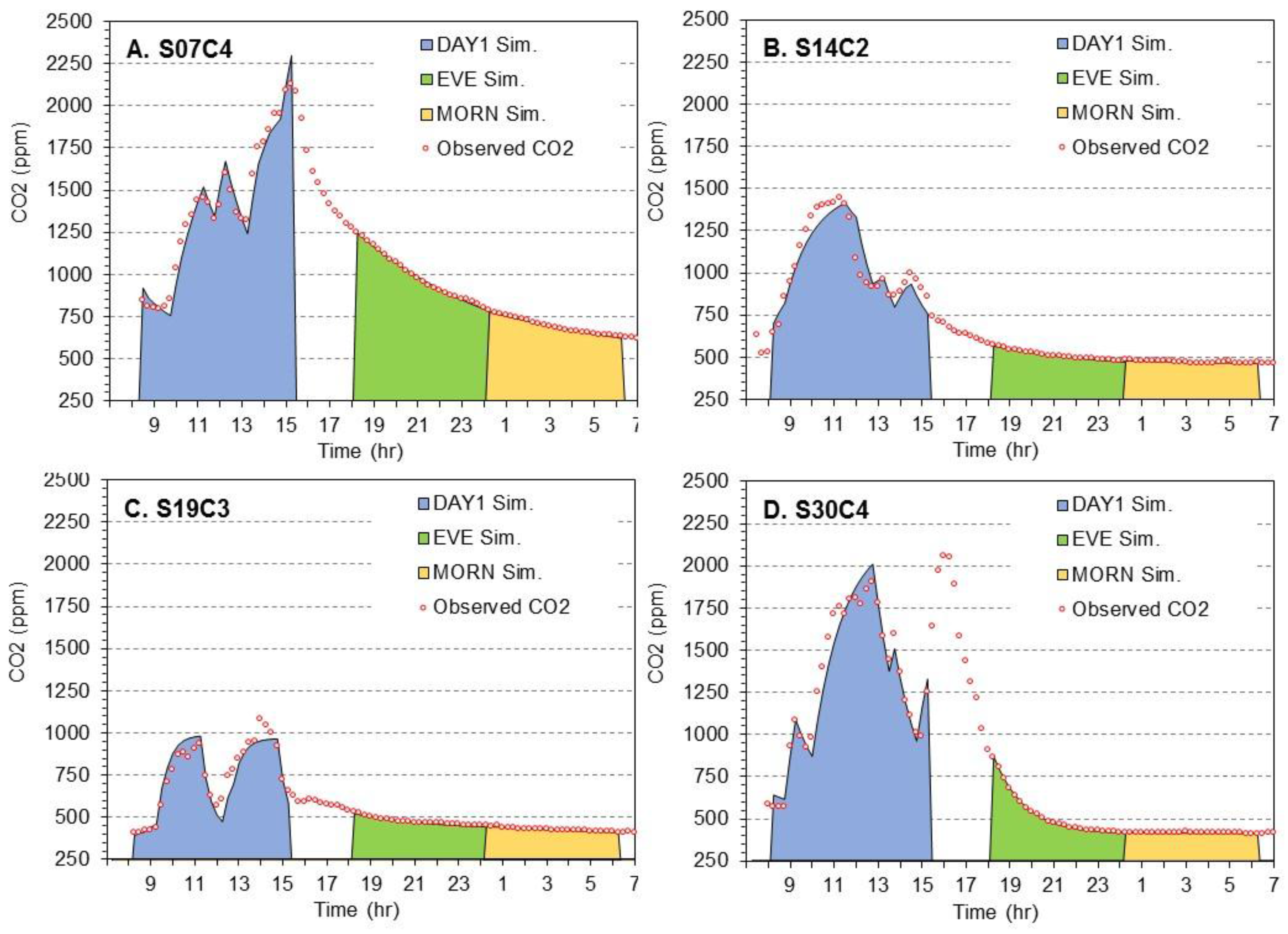
3.1. Comparison of Classrooms
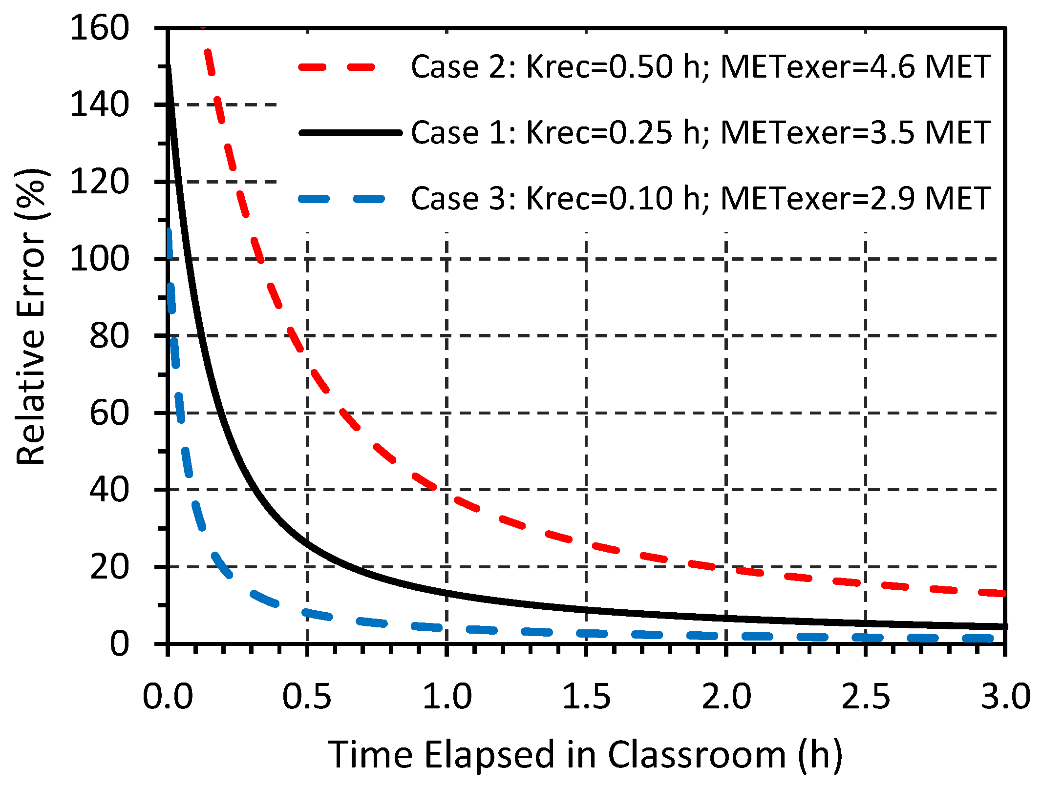
3.2. Effect of Post-Exercise Recovery
3.3. Evaluation of the Methods
3.4. Limitations
4. Conclusions
Supplementary Materials
Acknowledgments
Conflicts of Interest
References
- Haverinen-Shaughnessy, U.; Moschandreas, D.J.; Shaughnessy, R.J. Association between substandard classroom ventilation rates and students’ academic achievement. Indoor Air 2011, 21, 121–131. [Google Scholar] [CrossRef] [PubMed]
- Shendell, D.G.; Prill, R.; Fisk, W.J.; Apte, M.G.; Blake, D.; Faulkner, D. Associations between classroom CO2 concentrations and student attendance in Washington and Idaho. Indoor Air 2004, 14, 333–341. [Google Scholar] [CrossRef] [PubMed]
- Wargocki, P.; Wyon, D.P. The effects of outdoor air supply rate and supply air filter condition in classrooms on the performance of schoolwork by children (rp-1257). HVAC&R Res. 2007, 13, 165–191. [Google Scholar]
- Sundell, J.; Bronswijk, V.J.; Dijken, V.F. Indoor environment and pupils’ health in primary schools. Build. Res. Inform. 2006, 34, 437–446. [Google Scholar]
- Sundell, J.; Levin, H.; Nazaroff, W.W.; Cain, W.S.; Fisk, W.J.; Grimsrud, D.T.; Gyntelberg, F.; Li, Y.; Persily, A.K.; Pickering, A.C.; et al. Ventilation rates and health: Multidisciplinary review of the scientific literature. Indoor Air 2011, 21, 191–204. [Google Scholar] [CrossRef] [PubMed]
- Mendell, M.J.; Eliseeva, E.A.; Davies, M.M.; Spears, M.; Lobscheid, A.; Fisk, W.J.; Apte, M.G. Association of classroom ventilation with reduced illness absence: A prospective study in California elementary schools. Indoor Air 2013, 23, 515–528. [Google Scholar] [CrossRef] [PubMed]
- Rosbach, J.T.M.; Vonk, M.; Duijm, F.; van Ginkel, J.T.; Gehring, U.; Brunekreef, B. A ventilation intervention study in classrooms to improve indoor air quality: The FRESH study. Environ. Health 2013, 12, 110. [Google Scholar] [CrossRef] [PubMed]
- Haverinen-Shaughnessy, U.; Shaughnessy, R.J. Effects of classroom ventilation rate and temperature on students’ test scores. PLoS ONE 2015, 10, e0136165. [Google Scholar] [CrossRef] [PubMed]
- Gaihre, S.; Semple, S.; Miller, J.; Fielding, S.; Turner, S. Classroom carbon dioxide concentration, school attendance, and educational attainment. J. Sch. Health 2014, 84, 569–574. [Google Scholar] [CrossRef] [PubMed]
- Chatzidiakou, L.; Mumovic, D.; Summerfield, A.J. What do we know about indoor air quality in school classrooms? A critical review of the literature. Intell. Build. Int. 2012, 4, 228. [Google Scholar] [CrossRef]
- Pérez-Lombard, L.; Ortiz, J.; Pout, C. A review on buildings energy consumption information. Energy Build. 2008, 40, 394–398. [Google Scholar] [CrossRef]
- ASHRAE. ANSI/ASHRAE Standard 62.1-2013, Ventilation for Acceptable Indoor Air Quality; American Society of Heating, Refrigerating and Air-Conditioning Engineers, Inc.: Atlanta, GA, USA, 2013. [Google Scholar]
- Persily, A.K. Field measurement of ventilation rates. Indoor Air 2016, 26, 97–111. [Google Scholar] [CrossRef] [PubMed]
- Persily, A.K.; Gorfain, J.; Brunner, G. Survey of ventilation rates in office buildings. Build. Res. Inform. 2006, 34, 459–466. [Google Scholar] [CrossRef]
- Sherman, M.H. Tracer-gas techniques for measuring ventilation in a single zone. Build. Environ. 1990, 25, 365–374. [Google Scholar] [CrossRef]
- ASTM. Standard Test Method for Determining Air Change in a Single Zone by Means of a Tracer Gas Dilution; ASTM International: West Conshohocken, PA, USA, 2011. [Google Scholar]
- ISO. ISO 12569:2012: Thermal Performance of Buildings and Materials—Determination of Specific Airflow Rate in Buildings—Tracer Gas Dilution Method; International Organization for Standardization: Geneva, Switzerland, 2012; p. 54. [Google Scholar]
- Etheridge, D. Natural Ventilation of Buildings: Theory, Measurement and Design; John Wiley & Sons Inc./Wiley Wiley-Blackwell: West Sussex, UK, 2012. [Google Scholar]
- Bekö, G.; Gustavsen, S.; Frederiksen, M.; Bergsøe, N.C.; Kolarik, B.; Gunnarsen, L.; Toftum, J.; Clausen, G. Diurnal and seasonal variation in air exchange rates and interzonal airflows measured by active and passive tracer gas in homes. Build. Environ. 2016, 104, 178–187. [Google Scholar] [CrossRef]
- Chatzidiakou, E. Is CO2 A Good Proxy for Indoor Air Quality in School Classrooms? ProQuest Dissertations Publishing: London, UK, 2014. [Google Scholar]
- Hänninen, O.; Shaughnessy, R.; Turk, B.; Egorov, A. Evaluation of Ventilation Rates in European Schools Using CO2 Measurements as Part of a Proposed WHO School Survey; Healthy Buildings: Brisbane, Australia, 2012. [Google Scholar]
- Scheff, P.A.; Paulius, V.K.; Huang, S.W.; Conroy, L.M. Indoor air quality in a middle school, part I: Use of CO2 as a tracer for effective ventilation. Appl. Occup. Environ. Hyg. 2000, 15, 824–834. [Google Scholar] [CrossRef] [PubMed]
- Smith, P.N. Determination of ventilation rates in occupied buildings from metabolic CO2 concentrations and production rates. Build. Environ. 1988, 23, 95–102. [Google Scholar] [CrossRef]
- ASTM. Standard Guide for Using Indoor Carbon Dioxide Concentrations to Evaluate Indoor Air Quality and Ventilation; ASTM International: West Conshohocken, PA, USA, 2012. [Google Scholar]
- Hänninen, O. Novel second-degree solution to single zone mass-balance equation improves the use of build-up data in estimating ventilation rates in classrooms. J. Chem. Health Saf. 2013, 20, 14–19. [Google Scholar] [CrossRef]
- Mudarri, D.H. Potential correction factors for interpreting CO2 measurements in buildings. ASHRAE Trans. 1997, 103, 244–254. [Google Scholar]
- Carrilho, J.D.; Mateus, M.; Batterman, S.; da Silva, M.G. Air exchange rates from atmospheric CO2 daily cycle. Energy Build. 2015, 92, 188–194. [Google Scholar] [CrossRef] [PubMed]
- Hänninen, O.O.; Lebret, E.; Ilacqua, V.; Katsouyanni, K.; Künzli, N.; Srám, R.J.; Jantunen, M. Infiltration of ambient PM2.5 and levels of indoor generated non-ETS PM2.5 in residences of four European cities. Atmos. Environ. 2004, 38, 6411–6423. [Google Scholar]
- ASTM. E779-10 Standard Test. Method for Determining Air Leakage Rate by Fan Pressurization; American Society for Testing and Materials: West Conshohocken, PA, USA, 2010. [Google Scholar]
- Du, L.; Batterman, S.; Godwin, C.; Chin, J.-Y.; Parker, E.; Breen, M.; Brakefield, W.; Robins, T.; Lewis, T. Air change rates and interzonal flows in residences, and the need for multi-zone models for exposure and health analyses. Int. J. Environ. Res. Public Health 2012, 9, 4639–4662. [Google Scholar] [CrossRef] [PubMed]
- Carrer, P.; Wargocki, P.; Fanetti, A.; Bischof, W.; De Oliveira Fernandes, E.; Hartmann, T.; Kephalopoulos, S.; Palkonen, S.; Seppänen, O. What does the scientific literature tell us about the ventilation-health relationship in public and residential buildings? Build. Environ. 2015, 94, 273–286. [Google Scholar] [CrossRef]
- Hänninen, O. Combining CO2 Data from Ventilation Phases Improves Estimation of Air Exchange Rates; Healthy Buildings: Brisbane, Australia, 2012. [Google Scholar]
- WHO. Methods for Monitoring Indoor Air Quality in Schools: Report from the Meeting 4–5 April 2011 Bonn, Germany; World Health Organization: Copenhagen, Denmark, 2011; p. 32. [Google Scholar]
- George, K.; Ziska, L.H.; Bunce, J.A.; Quebedeaux, B. Elevated atmospheric CO2 concentration and temperature across an urban-rural transect. Atmos. Environ. 2007, 41, 7654–7665. [Google Scholar] [CrossRef]
- Yasuda, T.; Yonemura, S.; Tani, A. Comparison of the characteristics of small commercial NDIR CO2 sensor models and development of a portable CO2 measurement device. Sensors 2012, 12, 3641–3655. [Google Scholar] [CrossRef] [PubMed]
- Batterman, S.; Su, F.-C.; Wald, A.; Watkins, F.; Godwin, C.; Thun, T. Ventilation rates in recently constructed U.S. elementary school classrooms. Indoor Air 2017. under review. [Google Scholar]
- Breen, M.S.; Schultz, B.D.; Sohn, M.D.; Long, T.; Langstaff, J.; Williams, R.; Isaacs, K.; Meng, Q.Y.; Stallings, C.; Smith, L. A review of air exchange rate models for air pollution exposure assessments. J. Expo. Sci. Environ. Epidemiol. 2014, 24, 555–563. [Google Scholar] [CrossRef] [PubMed]
- Lawrence, T.M. Selecting CO2 criteria for outdoor air monitoring. ASHRAE J. 2008, 50, 18. [Google Scholar]
- Morse, R.G.; Haas, P.; Lattanzio, S.M.; Zehnter, D.; Divine, M. A cross-sectional study of schools for compliance to ventilation rate requirements. J. Chem. Health Saf. 2009, 16, 4–10. [Google Scholar] [CrossRef]
- You, Y.; Niu, C.; Zhou, J.; Liu, Y.; Bai, Z.; Zhang, J.; He, F.; Zhang, N. Measurement of air exchange rates in different indoor environments using continuous CO2 sensors. J. Environ. Sci. 2012, 24, 657–664. [Google Scholar] [CrossRef]
- Turanjanin, V.; Vutiaevic, B.; Jovanovic, M.; La Mirkov, N.; Lazovic, I. Indoor CO2 measurements in Serbian schools and ventilation rate calculation. Energy 2014, 77, 290–296. [Google Scholar] [CrossRef]
- Mundt, E.; Mathisen, H.M.; Nielsen, P.V.; Moser, A. Ventilation Effectiveness; REHVA Federation of European Heating Ventilation and Air Conditioning Associations: Brussels, Belgium, 2004. [Google Scholar]
- Canha, N.; Mandin, C.; Ramalho, O.; Wyart, G.; Ribéron, J.; Dassonville, C.; Hänninen, O.; Almeida, S.M.; Derbez, M. Assessment of ventilation and indoor air pollutants in nursery and elementary schools in France. Indoor Air 2016, 26, 350–365. [Google Scholar] [CrossRef] [PubMed]
- Hänninen, O.; Canha, N.; Dume, I.; Deliu, A.; Mata, E.; Egorov, A. P-217. Epidemiology 2012, 23, 1. [Google Scholar] [CrossRef]
- Penman, J.M. An experimental determination of ventilation rate in occupied rooms using atmospheric carbon dioxide concentration. Build. Environ. 1980, 15, 45–47. [Google Scholar] [CrossRef]
- Mumovic, D.; Palmer, J.; Davies, M.; Orme, M.; Ridley, I.; Oreszczyn, T.; Judd, C.; Critchlow, R.; Medina, H.A.; Pilmoor, G.; et al. Winter indoor air quality, thermal comfort and acoustic performance of newly built secondary schools in England. Build. Environ. 2009, 44, 1466–1477. [Google Scholar] [CrossRef]
- Santamouris, M.; Synnefa, A.; Asssimakopoulos, M.; Livada, I.; Pavlou, K.; Papaglastra, M.; Gaitani, N.; Kolokotsa, D.; Assimakopoulos, V. Experimental investigation of the air flow and indoor carbon dioxide concentration in classrooms with intermittent natural ventilation. Energy Build. 2008, 40, 1833–1843. [Google Scholar] [CrossRef]
- National Center for Health Statistics. Percentile Data Files with LMS Values, CDC Growth Charts. Available online: http://www.cdc.gov/growthcharts/percentile_data_files.htm (accessed on 1 October 2016).
- U.S. Environmental Protection Agency. Exposure Factors Handbook: 2011 Edition; U.S. Environmental Protection Agency: Washington, DC, USA, 2011.
- Saint-Maurice, P.F.; Kim, Y.; Welk, G.J.; Gaesser, G.A. Kids are not little adults: What MET threshold captures sedentary behavior in children? Eur. J. Appl. Physiol. Occup. Phys. 2016, 116, 29–38. [Google Scholar] [CrossRef] [PubMed]
- Ridley, K.; Ainsworth, B.E.; Olds, T.S. Development of a compendium of energy expenditures for youth. Int. J. Behav. Nutr. Phys. Act. 2008, 5, 45. [Google Scholar] [CrossRef] [PubMed]
- Ainsworth, B.E.; Haskell, W.L.; Herrmann, S.D.; Meckes, N.; Bassett, D.R., Jr.; Tudor-Locke, C.; Greer, J.L.; Vezina, J.; Whitt-Glover, M.C.; Leon, A.S. 2011 compendium of physical activities: A second update of codes and MET values. Med. Sci. Sports Exerc. 2011, 43, 1575–1581. [Google Scholar] [CrossRef] [PubMed]
- Buchheit, M.; Laursen, P.B.; Ratel, S.; Duché, P. Postexercise heart rate recovery in children: Relationship with power output, blood pH, and lactate. Appl. Physiol. Nutr. Metab. 2010, 35, 142–150. [Google Scholar] [CrossRef] [PubMed]
- Compher, C.; Frankenfield, D.; Keim, N.; Roth-Yousey, L. Best practice methods to apply to measurement of resting metabolic rate in adults: A systematic review. J. Am. Diet. Assoc. 2006, 106, 881–903. [Google Scholar] [CrossRef] [PubMed]
- Laforgia, J.; Withers, R.T.; Gore, C.J. Effects of exercise intensity and duration on the excess post-exercise oxygen consumption. J. Sports Sci. 2006, 24, 1247–1264. [Google Scholar] [CrossRef] [PubMed]


| Grade Level | Activity (MET) | Age Range | Weight | Height | Surface Area | CO2 Emissions | ||||||
|---|---|---|---|---|---|---|---|---|---|---|---|---|
| Start (Year) | End (Year) | Boys (kg) | Girls (kg) | Boys (cm) | Girls (cm) | Boys (m2) | Girls (m2) | Boys (L/min) | Girls (L/min) | Average (L/min) | ||
| PK | 1.4 | 4 | 5 | 18.4 | 18.0 | 108.9 | 107.7 | 0.74 | 0.73 | 0.149 | 0.146 | 0.147 |
| PK–K | 1.4 | 4 | 6 | 19.6 | 19.1 | 112.1 | 111.2 | 0.78 | 0.77 | 0.156 | 0.153 | 0.155 |
| K | 1.4 | 5 | 6 | 20.7 | 20.3 | 115.4 | 114.7 | 0.81 | 0.80 | 0.163 | 0.161 | 0.162 |
| K–1 | 1.4 | 5 | 7 | 21.9 | 21.5 | 118.5 | 118.0 | 0.85 | 0.84 | 0.170 | 0.169 | 0.169 |
| 1.0 | 1.4 | 6 | 7 | 23.1 | 22.8 | 121.7 | 121.4 | 0.89 | 0.88 | 0.178 | 0.176 | 0.177 |
| 1.5 | 1.4 | 6 | 8 | 24.4 | 24.3 | 124.8 | 124.4 | 0.92 | 0.92 | 0.185 | 0.184 | 0.185 |
| 2.0 | 1.4 | 7 | 8 | 25.7 | 25.7 | 127.8 | 127.5 | 0.96 | 0.96 | 0.192 | 0.192 | 0.192 |
| 2.5 | 1.4 | 7 | 9 | 27.2 | 27.4 | 130.6 | 130.2 | 1.00 | 1.00 | 0.200 | 0.200 | 0.200 |
| 3.0 | 1.4 | 8 | 9 | 28.6 | 29.1 | 133.4 | 132.9 | 1.04 | 1.04 | 0.208 | 0.209 | 0.208 |
| 3.5 | 1.4 | 8 | 10 | 30.3 | 31.0 | 136.0 | 135.5 | 1.08 | 1.09 | 0.216 | 0.217 | 0.217 |
| 4.0 | 1.4 | 9 | 10 | 32.0 | 33.0 | 138.6 | 138.1 | 1.12 | 1.13 | 0.224 | 0.226 | 0.225 |
| 4.5 | 1.4 | 9 | 11 | 34.0 | 35.1 | 141.1 | 141.2 | 1.16 | 1.18 | 0.233 | 0.236 | 0.235 |
| 5.0 | 1.4 | 10 | 11 | 36.0 | 37.2 | 143.6 | 144.2 | 1.21 | 1.23 | 0.242 | 0.246 | 0.244 |
| 5.5 | 1.4 | 10 | 12 | 38.3 | 39.4 | 146.5 | 147.6 | 1.26 | 1.28 | 0.252 | 0.256 | 0.254 |
| 6.0 | 1.4 | 11 | 12 | 40.6 | 41.6 | 149.3 | 151.0 | 1.31 | 1.33 | 0.262 | 0.267 | 0.264 |
| 6.5 | 1.4 | 11 | 13 | 43.1 | 43.7 | 152.8 | 153.8 | 1.36 | 1.38 | 0.273 | 0.276 | 0.274 |
| 7.0 | 1.4 | 12 | 13 | 45.6 | 45.7 | 156.2 | 156.7 | 1.42 | 1.42 | 0.284 | 0.285 | 0.285 |
| 7.5 | 1.4 | 12 | 14 | 48.3 | 47.5 | 159.9 | 158.4 | 1.48 | 1.46 | 0.296 | 0.292 | 0.294 |
| 8.0 | 1.4 | 13 | 14 | 51.0 | 49.2 | 163.6 | 160.1 | 1.54 | 1.49 | 0.308 | 0.299 | 0.303 |
| 9.0 | 1.4 | 14 | 15 | 56.2 | 51.9 | 169.5 | 161.7 | 1.64 | 1.54 | 0.329 | 0.308 | 0.319 |
| 10.0 | 1.4 | 15 | 16 | 60.8 | 53.8 | 173.2 | 162.5 | 1.73 | 1.57 | 0.346 | 0.314 | 0.330 |
| 11.0 | 1.4 | 16 | 17 | 64.4 | 55.1 | 175.1 | 162.9 | 1.78 | 1.58 | 0.357 | 0.317 | 0.337 |
| 12.0 | 1.4 | 17 | 18 | 67.1 | 56.2 | 176.1 | 163.1 | 1.82 | 1.60 | 0.365 | 0.320 | 0.343 |
| Mixed | 1.4 | 5 | 11 | 28.8 | 29.3 | 129.2 | 129.4 | 1.02 | 1.02 | 0.203 | 0.205 | 0.204 |
| Adult | 1.7 | 20 | 70 | 88.2 | 75.6 | 176.8 | 163.3 | 2.05 | 1.82 | 0.500 | 0.442 | 0.471 |
| ID | Room, School, HVAC, Weather | HVAC Description and Calculated Air Change Rate |
|---|---|---|
| S07C4 | Large mixed-grade classroom (299 m3) in a midsize conventional building (9012 m2, 29 classrooms) constructed in 2005. School day: Temp: 13 (11–15) °C Wind speed: 9 (7–11) m/s Eve + Morn: Temp: 10 (9–11) °C Wind speed: 12 (8–15) m/s | Building uses conventional variable air volume (VAV) system with central air handling units (AHUs) and energy recovery (ER). Five ceiling mounted diffusers in the room collectively discharge 142 to 519 L·s−1 (minimum of 236 L·s−1 during the heating season) with a minimum of 30% outside air (OA). Given building/HVAC data, estimated air change rates are 0.85 to 1.45 h−1 in the heating season. |
| S14C2 | Large prekindergarten/ kindergarten classroom (322 m3) in a smaller (7430 m2, 22 classrooms) and newer building constructed in 2011. School day: Temp: 5 (4–5) °C Wind speed: 5 (4–6) m/s Eve + Morn: Temp: 8 (5–9) °C Wind speed: 7 (5–12) m/s | Classroom uses vertical unit ventilator (UV) with multiple fan speeds, fully adjustable dampers, and rated capacity of 755 L·s−1. UV had dirty filters (reportedly changed twice yearly). Assuming a minimum flow of 40% of capacity and a minimum of 30% OA, the air change rate is 1.01 h−1. |
| S19C3 | 2nd grade classroom (213 m3) in a midsize (10,400 m2, 36 classrooms) EnergyStar building constructed in 2005. School day: Temp: −11 (−17–−6) °C Wind speed: 6 (3–8) m/s Eve + Morn: Temp: −12 (−17–−8) °C Wind speed: 5 (3–8) m/s | Building uses geothermal heat pumps for each classroom and centralized make-up air (100% OA) discharged through four ceiling diffusers. Design drawings show the maximum OA flow rate to the room of 566 L·s−1. Assuming a minimum of 30% of rated flow, the air change rate is 2.87 h−1; at maximum flow, the rate is 9.56 h−1. |
| S30C4 | Large 4th grade classroom (281 m3) in a smaller (5760 m2, 21 classrooms) EnergyStar building that has had several expansions since original construction in 1975. Complete building renovation in 2007. School day: Temp: −6 (−7–−4) °C Wind speed: 4 (3–6) m/s Eve + Morn: Temp: −4 (−6–−2) °C Wind speed: 6 (4–7) m/s | Building uses a UV in each classroom with a maximum flow of 519 L·s−1 discharged through four ceiling diffusers. Assuming a minimum of 50% of the rated flow and 30% OA, the air change rate is 1.00 h−1; at maximum flow, the air change rate is 2.00 h−1. |
| Period of Day | Method | Conventional Buildings | EnergyStar Buildings | ||
|---|---|---|---|---|---|
| S07C4 | S14C2 | S19C3 | S30C4 | ||
| School day (occupied) | |||||
| Transient mass balance | 0.51 | 0.77 | 2.42 | 0.70 | |
| Steady-state | 0.52 | 0.67 | 1.41 | 0.80 | |
| Build-up-3 point | 0.31 | 0.77 | 0.70 | 0.22 | |
| Build-up-implicit | 0.43 | 0.57 | 2.10 | 0.62 | |
| Build-up-ASTM | 0.52 | 0.68 | 13.19 | 1.34 | |
| Evening (unoccupied) | |||||
| Transient mass balance | 0.14 | 0.18 | 0.27 | 0.72 | |
| Decay | 0.13 | 0.13 | 0.17 | 0.57 | |
| Early morning (unoccupied) | |||||
| Transient mass balance | 0.098 | 0.057 | 0.113 | 0.011 | |
| Decay | 0.085 | 0.025 | 0.322 | 0.053 | |
© 2017 by the author. Licensee MDPI, Basel, Switzerland. This article is an open access article distributed under the terms and conditions of the Creative Commons Attribution (CC BY) license ( http://creativecommons.org/licenses/by/4.0/).
Share and Cite
Batterman, S. Review and Extension of CO2-Based Methods to Determine Ventilation Rates with Application to School Classrooms. Int. J. Environ. Res. Public Health 2017, 14, 145. https://doi.org/10.3390/ijerph14020145
Batterman S. Review and Extension of CO2-Based Methods to Determine Ventilation Rates with Application to School Classrooms. International Journal of Environmental Research and Public Health. 2017; 14(2):145. https://doi.org/10.3390/ijerph14020145
Chicago/Turabian StyleBatterman, Stuart. 2017. "Review and Extension of CO2-Based Methods to Determine Ventilation Rates with Application to School Classrooms" International Journal of Environmental Research and Public Health 14, no. 2: 145. https://doi.org/10.3390/ijerph14020145
APA StyleBatterman, S. (2017). Review and Extension of CO2-Based Methods to Determine Ventilation Rates with Application to School Classrooms. International Journal of Environmental Research and Public Health, 14(2), 145. https://doi.org/10.3390/ijerph14020145