
Analysis of Sampling Methodologies for Noise Pollution Assessment and the Impact on the Population


Abstract
:1. Introduction
- Compare the applicability and predictive capacity of two sampling methods—the legislative road classification and the categorisation method—in the assessment of urban noise in a Chilean city.
- Compare both sampling methods in terms of the prediction of exposure levels and the percentage of people annoyed.
2. Methods
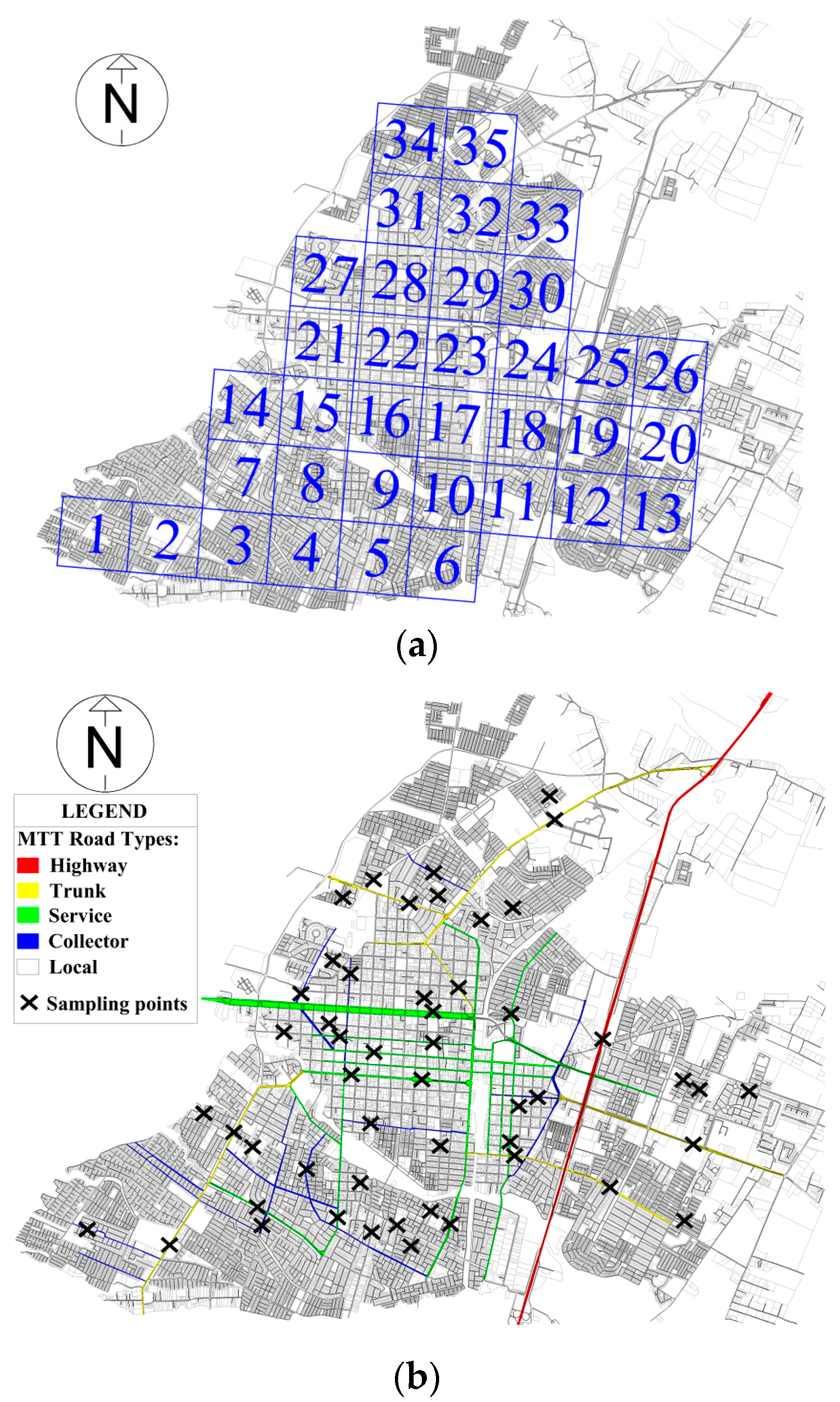
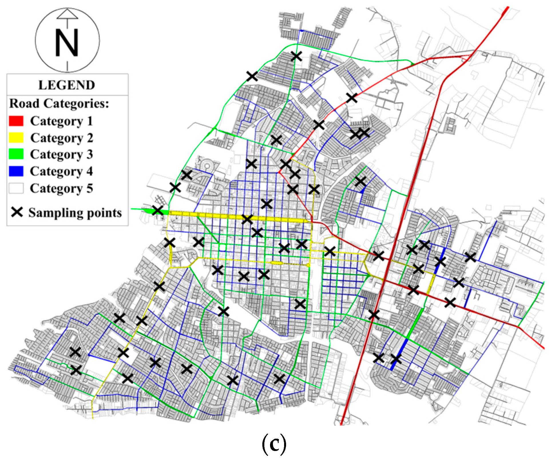
2.1. Grid Method
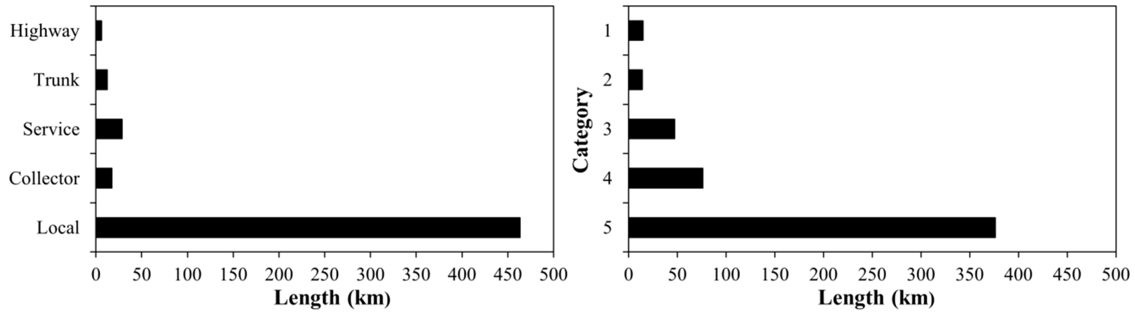
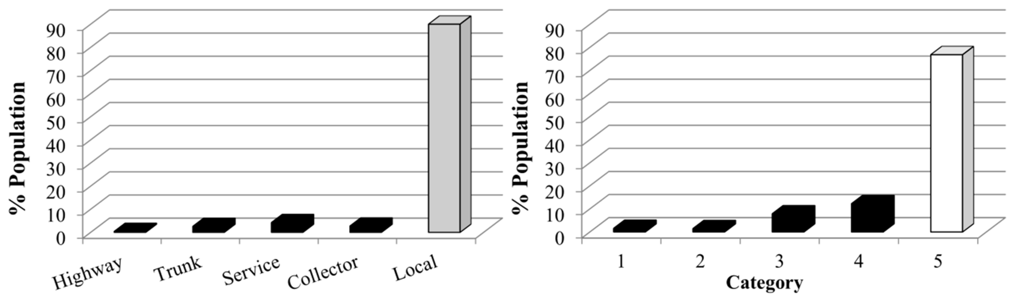
2.2. Road Types Established by the MTT
2.3. Categorisation Method
2.4. Measurement Procedure
2.5. Statistical Analysis
3. Results
3.1. Study of the Functioning of Sampling Methods
3.1.1. Grid Method
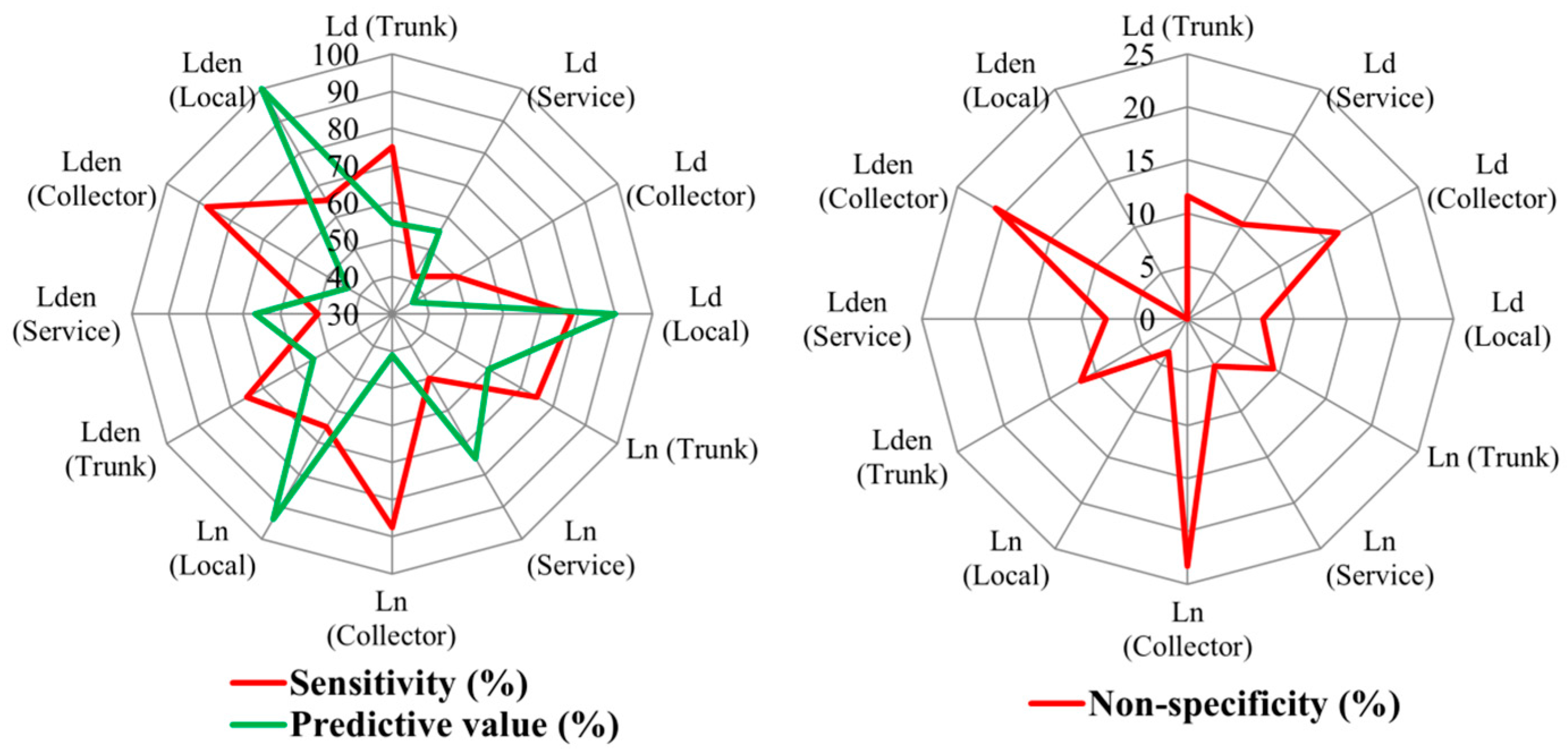
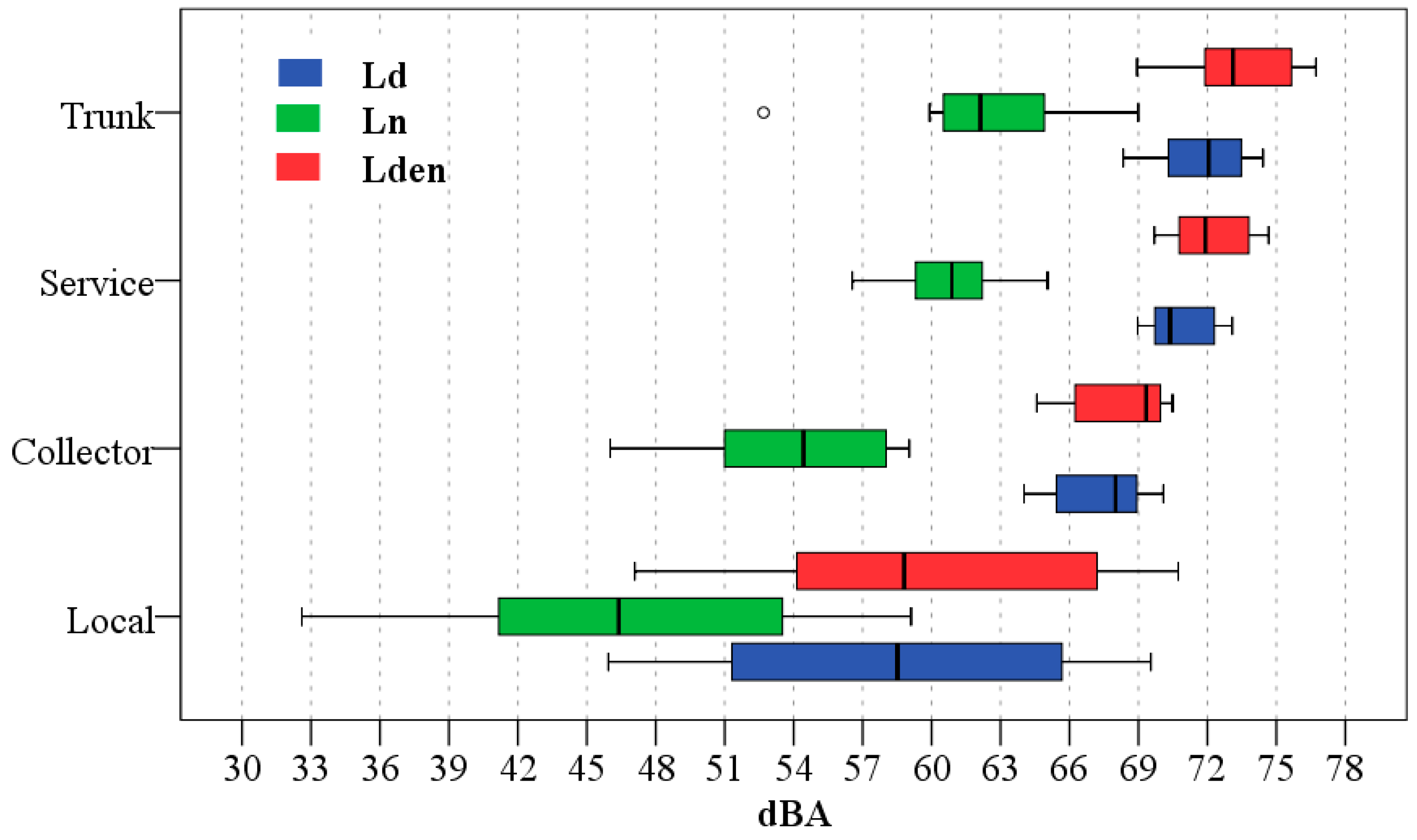
3.1.2. MTT Road Types
- Regarding the ROC sensitivity (%), which is a measure of the capacity to include previously assigned sampling points in the stratum, only the collector road type for Ln and Lden has values above 80%. The sensitivity has low percentages for the sound descriptors analysed, sometimes even lower than 50%, because of the presence of overlaps among trunk and service road types and the high variability of the local road type.
- Regarding the non-specificity (%), which measures the proportion of sampling points that were not initially assigned to a given stratum, but which the ROC analysis indicates belong to that stratum, only the local road type has values lower than 10% for all the sound descriptors. The collector road type also has high non-specificity values for all the sound descriptors, although it has high sensitivity values for Ln and Lden.
- Finally, with regard to the predictive values of the different road types (which represent the proportion of the sampling points that the ROC analysis assigned to the stratum that matched the road types to which they were initially assigned, relative to the total number of sampling points that the ROC analysis determined for the stratum) only the local road type has values above 80% for all the sound descriptors. The stratum predicted by the ROC analysis for local road types has a high percentage of sampling points that MTT had initially classified in this road type. However, other sampling points of local road types have high values and these points are classified in other road types according to ROC analysis. Therefore, the local road type has low sensitivity values.
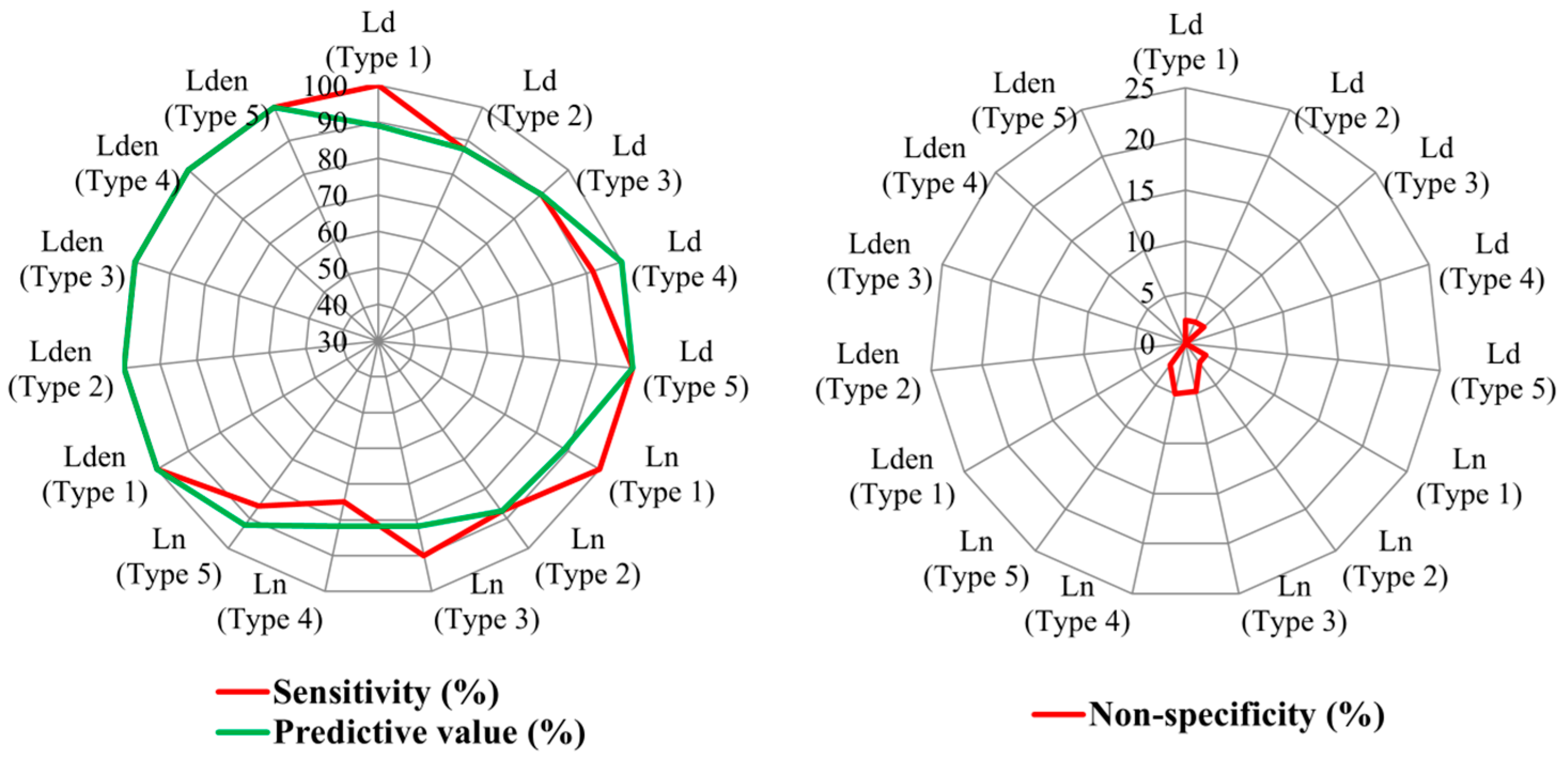
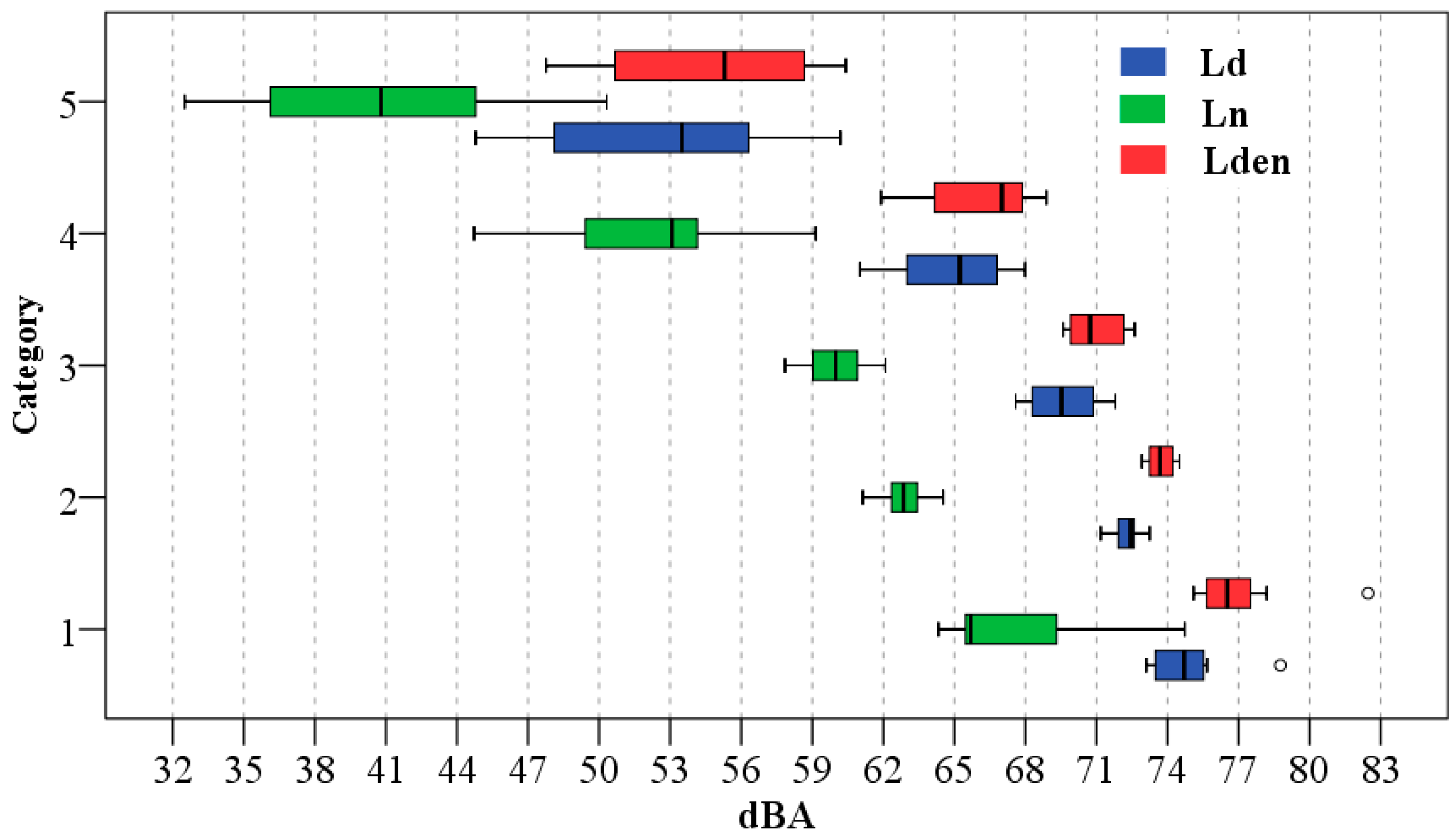
3.1.3. Categorisation Method
3.2. Predictive Capacity Analysis
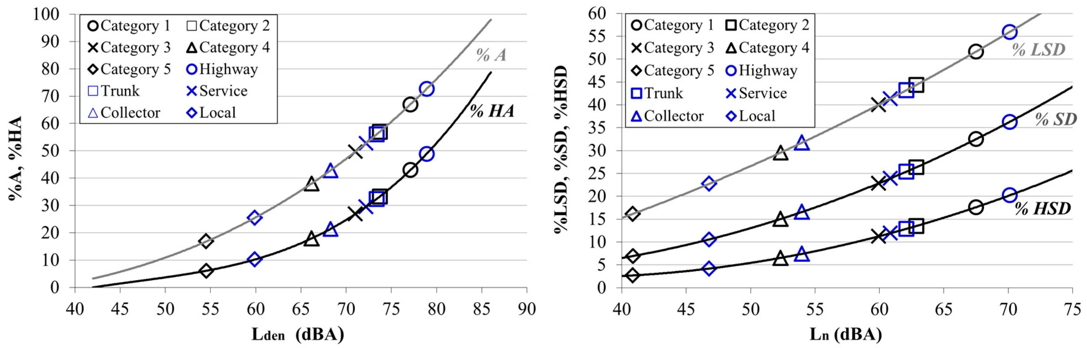
3.3. Calculation of Exposure Level and the Percentage of Annoyance
4. Discussion
5. Conclusions
Acknowledgments
Author Contributions
Conflicts of Interest
References
- World Health Organization. Burden of Disease from Environmental Noise—Quantification of Healthy Life Years Lost in Europe; WHO Regional Office for Europe: Copenhagen, Denmark, 2011. [Google Scholar]
- Marquis-Favre, C.; Premat, E.; Vallety, M. Noise and its effects—A review on qualitative aspects of sound: Part I: Notions and acoustic ratings. Acta Acust. 2005, 91, 613–625. [Google Scholar]
- Basner, M.; Babisch, W.; Davis, A.; Brink, M.; Clark, C.; Janssen, S.; Stansfeld, S. Auditory and non-auditory effects of noise on health. Lancet 2014, 383, 1325–1332. [Google Scholar] [CrossRef]
- Stansfeld, S.A.; Matheson, M.P. Noise pollution: Non-auditory effects on health. Br. Med. Bull. 2003, 68, 243–257. [Google Scholar] [CrossRef] [PubMed]
- De Kluizenaar, Y.; Gansevoort, R.T.; Miedema, H.M.E.; de Jong, P.E. Hypertension and road traffic noise exposure. J. Occup. Environ. Med. 2007, 49, 484–492. [Google Scholar] [CrossRef] [PubMed]
- Pirrera, S.; de Valck, E.; Cluydts, R. Nocturnal road traffic noise: A review on its assessment and consequences on sleep and health. Environ. Int. 2010, 36, 492–498. [Google Scholar] [CrossRef] [PubMed]
- Rey Gozalo, G.; Barrigón Morillas, J.M.; Gómez Escobar, V. Analyzing nocturnal noise stratification. Sci. Total Environ. 2014, 479, 39–47. [Google Scholar] [CrossRef] [PubMed]
- Fields, J.M. Reactions to environmental noise in an ambient noise context in residential areas. J. Acoust. Soc. Am. 1998, 104, 2245–2260. [Google Scholar] [CrossRef]
- Guski, R.; Feldcher-Suhr, U.; Schuemer, R. The concept of noise annoyance: How international experts see it. J. Sound Vib. 1999, 223, 513–527. [Google Scholar] [CrossRef]
- Barrigón Morillas, J.M.; Gómez Escobar, V.; Méndez Sierra, J.A.; Vílchez-Gómez, R.; Vaquero, J.M. Effects of leisure activity related noise in residential zones. Build. Acoust. 2005, 12, 265–276. [Google Scholar] [CrossRef]
- King, R.P.; Davis, J.R. Community noise: Health effects and management. Int. J. Hyg. Environ. Health 2003, 206, 123–131. [Google Scholar] [CrossRef] [PubMed]
- Moudon, A.N. Real noise from the urban environment: How ambient community noise affects health and what can be done about it. Am. J. Prev. Med. 2009, 37, 167–171. [Google Scholar] [CrossRef] [PubMed]
- Dratva, J.; Zemp, E.; Dietrich, D.-F.; Bridevaux, P.-O.; Rochat, T.; Schindler, C.; Gerbase, M.W. Impact of road traffic noise annoyance on health-related quality of life: Results from a population based study. Qual. Life Res. 2010, 19, 37–46. [Google Scholar] [CrossRef] [PubMed]
- Brink, M. Parameters of well-being and subjective health and their relationship with residential traffic noise exposure—A representative evaluation in Switzerland. Environ. Int. 2011, 37, 723–733. [Google Scholar] [CrossRef] [PubMed]
- Braubach, M.; Tobollik, M.; Mudu, P.; Hiscock, R.; Chapizanis, D.; Sarigiannis, D.A.; Keuken, M.; Perez, L.; Martuzzi, M. Development of a quantitative methodology to assess the impacts of urban transport interventions and related noise on well-being. Int. J. Environ. Res. Public Health 2015, 12, 5792–5814. [Google Scholar] [CrossRef] [PubMed]
- Frei, P.; Mohler, E.; Röösli, M. Effect of nocturnal road traffic noise exposure and annoyance on objectiveand subjective sleep quality. Int. J. Hyg. Environ. Health 2014, 217, 188–195. [Google Scholar] [CrossRef] [PubMed]
- Mavanji, V.; Teske, J.A.; Billington, C.J.; Kotz, C.M. Partial sleep deprivation by environmental noise increases food intake and body weight in obesity-resistant rats. Obesity 2013, 2, 1396–1405. [Google Scholar] [CrossRef] [PubMed]
- Oftedal, B.; Krog, N.H.; Pyko, A.; Eriksson, C.; Graff-Iversen, S.; Haugen, M.; Schwarze, P.E.; Pershagen, G.; Aasvang, G.M. Road traffic noise and markers of obesity—A population-based study. Environ. Res. 2015, 138, 144–153. [Google Scholar] [CrossRef] [PubMed]
- Sørensen, M.; Andersen, Z.J.; Nordsborg, R.B.; Becker, T.; Tjønneland, A.; Overvad, K.; Raaschou-Nielsen, O. Long-term exposure to road traffic noise and incident diabetes: A cohort study. Environ. Health Perspect. 2013, 121, 217–222. [Google Scholar] [PubMed]
- Meisinger, C.; Heier, M.; Löwel, H.; Schneider, A.; Döring, A. Sleep duration and sleep complaints and risk of myocardial infarction in middle-aged men and women from the general population: The Monica/Kora Augsburg cohort study. Sleep 2007, 30, 1121–1127. [Google Scholar] [PubMed]
- Bluhm, G.L.; Berglind, N.; Nordling, E.; Rosenlund, M. Road traffic noise and hypertension. Occup. Environ. Med. 2007, 64, 122–126. [Google Scholar] [CrossRef] [PubMed]
- European Commision. Directive 2002/49/EC of the European Parliament and of the Council of 25 June 2002 relating to the assessment and management of environmental noise. Off. J. Eur. Communities 2002, 18, 12–25. [Google Scholar]
- Dekoninck, L.; Botteldooren, D.; Panis, L.I. Using city-wide mobile noise assessments to estimate bicycle trip annual exposure to Black Carbon. Environ. Int. 2015, 85, 192–201. [Google Scholar] [CrossRef] [PubMed]
- Stansfeld, S.A. Noise effects on health in the context of air pollution exposure. Int. J. Environ. Res. Public Health 2015, 12, 12735–12760. [Google Scholar] [CrossRef] [PubMed]
- Banerjee, D.; Chakraborty, S.K.; Bhattacharyya, S.; Gangopadhyay, A. Evaluation and analysis of road traffic noise in Asansol: An industrial town of eastern India. Int. J. Environ. Res. Public Health 2008, 5, 165–171. [Google Scholar] [CrossRef] [PubMed]
- Seong, J.C.; Park, T.H.; Ko, J.H.; Chang, S.I.; Kim, M.; Holt, J.B.; Mehdi, M.R. Modeling of road traffic noise and estimated human exposure in Fulton County, Georgia, USA. Environ. Int. 2011, 37, 1336–1341. [Google Scholar] [CrossRef] [PubMed]
- Dintrans, A.; Préndez, M. A method of assessing measures to reduce road traffic noise: A case study in Santiago, Chile. Appl. Acoust. 2013, 74, 1486–1491. [Google Scholar] [CrossRef]
- Lee, J.; Gu, J.; Park, H.; Yun, H.; Kim, S.; Lee, W.; Han, J.; Cha, J.S. Estimation of populations exposed to road traffic noise in districts of Seoul metropolitan area of Korea. Int. J. Environ. Res. Public Health 2014, 11, 2729–2740. [Google Scholar] [CrossRef] [PubMed]
- Mapcity. Available online: http://mapcity.com/mapaderuido#t=1 (accessed on 2 February 2016).
- European Commission Working Group–Assessment of Exposure to Noise. Good Practice Guide for Strategic Noise Mapping and the Production Associated Data on Noise Exposure, version 2; European Commission: Brussels, Belgium, 2007. [Google Scholar]
- Environmental Protection Agency. Guidance Note for Strategic Noise Mapping for the Environmental Noise Regulations 2006, Version 2; Environmental Protection Agency: Wexford, Ireland, 2011. [Google Scholar]
- Kang-Ting, T.; Min-Der, L.; Yen-Hua, C. Noise mapping in urban environments: A Taiwan study. Appl. Acoust. 2009, 70, 964–972. [Google Scholar]
- Gómez Escobar, V.; Barrigón Morillas, J.M.; Rey Gozalo, G.; Vílchez-Gómez, R.; Carmona del Río, F.J.; Méndez Sierra, J.A. Analysis of the grid sampling method for noise mapping. Arch. Acoust. 2012, 37, 499–514. [Google Scholar] [CrossRef]
- Del Carmona Río, F.J.; Gómez Escobar, V.; Trujillo Carmona, J.; Vílchez-Gómez, R.; Méndez Sierra, J.A.; Rey Gozalo, G.; Barrigón Morillas, J.M. A street categorization method to study urban noise: The valladolid (Spain) study. Environ. Eng. Sci. 2011, 28, 811–817. [Google Scholar] [CrossRef]
- Romeu, J.; Genescà, M.; Pàmies, T.; Jiménez, S. Street categorization for the estimation of day levels using short-term measurements. Appl. Acoust. 2011, 72, 569–577. [Google Scholar] [CrossRef]
- Barrigón Morillas, J.M.; Ortiz-Caraballo, C.; Prieto Gajardo, C. The temporal structure of pollution levels in developed cities. Sci. Total Environ. 2015, 517, 31–37. [Google Scholar] [CrossRef] [PubMed]
- Ko, J.H.; Chang, S.I.; Lee, B.C. Noise impact assessment by utilizing noise map and GIS: A case study in the city of Chungju, Republic of Korea. Appl. Acoust. 2011, 72, 544–550. [Google Scholar] [CrossRef]
- Suárez, E.; Barros, J.L. Traffic noise mapping of the city of Santiago de Chile. Sci. Total Environ. 2014, 466, 539–546. [Google Scholar] [CrossRef] [PubMed]
- Zambon, G.; Benocci, R.; Brambilla, G. Cluster categorization of urban roads to optimize their noise monitoring. Environ. Monit. Assess. 2016, 188, 1–11. [Google Scholar] [CrossRef] [PubMed]
- Doygun, H.; Gurun, D.K. Analyzing and mapping spatial and temporal dynamics of urban traffic noise pollution: A case study in Kahramanmaras, Turkey. Environ. Monit. Assess. 2008, 142, 65–72. [Google Scholar] [CrossRef] [PubMed]
- Baloye, D.O.; Palamuleni, L.G. A comparative land use-based analysis of noise pollution levels in selected urban centers of Nigeria. Int. J. Environ. Res. Public Health 2015, 12, 12225–12246. [Google Scholar] [CrossRef] [PubMed]
- ISO 1996-2. Description, Measurement and Assessment of Environmental Noise, Part 2: Determination of Environmental Noise Levels; International Organization for Standardization: Geneva, Switzerland, 2007. [Google Scholar]
- Rey Gozalo, G.; Barrigón Morillas, J.M.; Gómez Escobar, V.; Vílchez-Gómez, R.; Méndez Sierra, J.A.; Carmona del Río, F.J.; Prieto Gajardo, C. Study of the categorisation method using long-term measurements. Arch. Acoust. 2013, 38, 397–405. [Google Scholar] [CrossRef]
- Rey Gozalo, G.; Barrigón Morillas, J.M.; Gómez Escobar, V. Urban streets functionality as a tool for urban pollution management. Sci. Total Environ. 2013, 461, 453–461. [Google Scholar] [CrossRef] [PubMed]
- Rey Gozalo, G.; Barrigón Morillas, J.M.; Prieto Gajardo, C. Urban noise functional stratification for estimating average annual sound level. J. Acoust. Soc. Am. 2015, 137, 3198–3208. [Google Scholar] [CrossRef] [PubMed]
- Ministerio de Transporte y Telecomunicaciones (MTT). Subsecretaría de Transporte. Secretaría Regional Ministerial VII Región del Maule. In Resolución 221 Exenta. Determina Red Vial Básica de la Comuna de Talca; Ministerio de Transporte y Telecomunicaciones: Talca, Chile, 1997. [Google Scholar]
- Rey Gozalo, G.; Barrigón Morillas, J.M.; Trujillo Carmona, J.; Montes González, D.; Atanasio Moraga, P.; Gómez Escobar, V.; Vílchez-Gómez, R.; Méndez Sierra, J.A.; Prieto Gajardo, C. Study on the relation between urban planning and noise level. Appl. Acoust. 2016, 111, 143–147. [Google Scholar] [CrossRef]
- Barrigón Morillas, J.M.; Gómez Escobar, V.; Méndez Sierra, J.A.; Vílchez-Gómez, R.; Trujillo Carmona, J. An environmental noise study in the city of Cáceres, Spain. Appl. Acoust. 2002, 63, 1061–1070. [Google Scholar] [CrossRef]
- Gaja, E.; Giménez, A.; Sancho, S.; Reig, A. Sampling techniques for the estimation of the annual equivalent noise level under urban traffic conditions. Appl. Acoust. 2003, 64, 43–53. [Google Scholar] [CrossRef]
- Kruskal, W.H.; Wallis, W.A. Use of ranks in one-criterion variance analysis. J. Am. Stat. Assoc. 1952, 47, 583–621. [Google Scholar] [CrossRef]
- Mann, H.B.; Whitney, D.R. On a test of whether one of two random variables is stochastically larger than the other. Ann. Math. Stat. 1947, 18, 50–60. [Google Scholar] [CrossRef]
- Holm, S. A simple sequentially rejective multiple test procedure. Scand. J. Stat. 1979, 6, 65–70. [Google Scholar]
- Barrigón Morillas, J.M.; Gómez Escobar, V.; Trujillo Carmona, J.; Méndez Sierra, J.M.; Vílchez-Gómez, R.; Carmona del Río, F.J. Analysis of the prediction capacity of a categorization method for urban noise assessment. Appl. Acoust. 2011, 72, 760–771. [Google Scholar] [CrossRef]
- Rey Gozalo, G.; Barrigón Morillas, J.M.; Gómez Escobar, V. Analysis of noise exposure in two small towns. Acta Acust. 2012, 98, 884–893. [Google Scholar] [CrossRef]
- Wilcoxon, F. Individual comparisons by ranking methods. Biometr. Bull. 1945, 1, 80–83. [Google Scholar] [CrossRef]
- Instituto Nacional de Estadística. Censos de Población y Vivienda—Censos Desde 1813 Hasta 2002; Instituto Nacional de Estadística: Santiago de Chile, Chile, 2010. [Google Scholar]
- ISO 1996-1. Description, Measurement and Assessment of Environmental Noise, Part 1: Basis Quantities and Assessment Procedures; International Organization for Standardization: Geneva, Switzerland, 2003. [Google Scholar]
- Miedema, H.M.E.; Oudshoorn, C.G.M. Annoyance from transportation noise: Relationships with exposure metrics DNL and DENL and their confidence intervals. Environ. Health Perspect. 2001, 109, 409–416. [Google Scholar] [CrossRef] [PubMed]
- Miedema, H.M.E.; Passchier-Vermeer, W.; Vos, H. Elements for a Position Paper on Night-Time Transportation Noise and Sleep Disturbance; TNO Inro: Delft, The Netherlands, 2003. [Google Scholar]
- Organization for Economic Cooperation and Development. Fighting Noise in 1990s; Alexandre, A., Barde, J.-P., Eds.; OECD Publications: Paris, France, 1991; p. 120. [Google Scholar]


| Grid | Ld (dBA) | Ln (dBA) | Lden (dBA) | Grid | Ld (dBA) | Ln (dBA) | Lden (dBA) | ||||||
|---|---|---|---|---|---|---|---|---|---|---|---|---|---|
| Me | IQR | Me | IQR | Me | IQR | Me | IQR | Me | IQR | Me | IQR | ||
| 1 | 51.4 | 12.8 | 44.0 | 16.8 | 53.1 | 13.9 | 19 | 62.7 | 21.8 | 54.9 | 23.0 | 63.6 | 17.8 |
| 2 | 59.4 | 17.8 | 53.0 | 21.7 | 63.0 | 18.2 | 20 | 51.7 | 11.9 | 44.5 | 10.7 | 55.3 | 5.6 |
| 3 | 64.9 | 9.3 | 53.1 | 17.9 | 65.5 | 10.2 | 21 | 64.7 | 14.4 | 52.3 | 23.3 | 65.7 | 15.3 |
| 4 | 64.9 | 14.6 | 50.3 | 24.7 | 65.5 | 15.9 | 22 | 72.3 | 5.8 | 62.2 | 7.3 | 73.8 | 5.4 |
| 5 | 53.2 | 16.6 | 41.8 | 21.1 | 53.9 | 16.4 | 23 | 67.2 | 17.2 | 59.0 | 19.9 | 69.1 | 16.8 |
| 6 | 48.7 | 4.7 | 43.4 | 3.3 | 52.4 | 3.4 | 24 | 62.2 | 13.9 | 52.8 | 20.0 | 63.8 | 14.4 |
| 7 | 62.5 | 22.2 | 52.9 | 24.1 | 63.2 | 16.9 | 25 | 55.2 | 22.0 | 49.2 | 12.9 | 58.9 | 17.6 |
| 8 | 69.0 | 20.0 | 59.0 | 10.3 | 70.3 | 14.2 | 26 | 51.8 | 11.3 | 43.8 | 6.5 | 55.3 | 6.2 |
| 9 | 61.0 | 21.5 | 50.6 | 20.1 | 62.1 | 21.1 | 27 | 64.7 | 15.4 | 51.5 | 11.0 | 65.7 | 14.0 |
| 10 | 50.3 | 5.4 | 42.3 | 3.7 | 52.5 | 3.8 | 28 | 69.7 | 8.5 | 58.4 | 11.2 | 70.5 | 8.6 |
| 11 | 56.7 | 16.4 | 47.7 | 15.1 | 58.6 | 15.6 | 29 | 66.4 | 19.0 | 51.5 | 26.1 | 67.1 | 19.5 |
| 12 | 57.3 | 12.0 | 51.5 | 19.3 | 60.8 | 11.9 | 30 | 61.4 | 8.1 | 45.2 | 17.0 | 61.8 | 9.4 |
| 13 | 55.1 | 11.3 | 47.0 | 12.1 | 57.9 | 7.5 | 31 | 60.7 | 23.9 | 47.9 | 23.6 | 61.9 | 22.9 |
| 14 | 55.3 | 10.1 | 35.8 | 10.5 | 55.8 | 4.0 | 32 | 57.5 | 22.3 | 41.7 | 19.3 | 58.4 | 20.6 |
| 15 | 62.2 | 24.6 | 53.8 | 25.3 | 63.3 | 19.3 | 33 | 60.1 | 12.6 | 47.1 | 16.0 | 61.4 | 12.5 |
| 16 | 71.6 | 16.3 | 61.0 | 18.7 | 73.1 | 16.5 | 34 | 62.1 | 21.3 | 50.3 | 21.4 | 63.4 | 20.4 |
| 17 | 58.4 | 17.8 | 49.6 | 19.7 | 60.1 | 18.4 | 35 | 51.0 | 18.6 | 41.6 | 14.5 | 53.3 | 17.4 |
| 18 | 65.7 | 14.9 | 58.6 | 15.7 | 67.9 | 14.9 | |||||||
| Ld | Road Types | Trunk | Service | Collector |
| Service | 0.343 | - | - | |
| Collector | 0.005 | 0.003 | - | |
| Local | <0.001 | <0.001 | 0.005 | |
| Ln | Road types | Trunk | Service | Collector |
| Service | 0.208 | - | - | |
| Collector | 0.009 | 0.002 | - | |
| Local | <0.001 | <0.001 | 0.046 | |
| Lden | Road types | Trunk | Service | Collector |
| Service | 0.270 | - | - | |
| Collector | 0.008 | <0.001 | - | |
| Local | <0.001 | <0.001 | 0.008 |
| Ld | Category | 1 | 2 | 3 | 4 |
| 2 | <0.001 | - | - | - | |
| 3 | <0.001 | <0.001 | - | - | |
| 4 | <0.001 | <0.001 | <0.001 | - | |
| 5 | <0.001 | <0.001 | <0.001 | <0.001 | |
| Ln | Category | 1 | 2 | 3 | 4 |
| 2 | 0.002 | - | - | - | |
| 3 | 0.001 | 0.002 | - | - | |
| 4 | 0.001 | 0.001 | 0.001 | - | |
| 5 | 0.001 | <0.001 | <0.001 | <0.001 | |
| Lden | Category | 1 | 2 | 3 | 4 |
| 2 | <0.001 | - | - | - | |
| 3 | <0.001 | <0.001 | - | - | |
| 4 | <0.001 | <0.001 | <0.001 | - | |
| 5 | <0.001 | <0.001 | <0.001 | <0.001 |
| Road Types | No. Points | εLd | εLn | εLden |
|---|---|---|---|---|
| Trunk | 13 | 1.3 * | 2.2 ** | 2.3 n.s. |
| Service | 13 | 1.3 * | 1.3 * | 1.5 * |
| Collector | 3 | 0.5 n.s. | 4.1 n.s. | 0.8 n.s. |
| Local | 74 | −1.0 n.s. | −0.3 n.s. | −0.6 n.s. |
| Category | No. Points | εLd | εLn | εLden |
|---|---|---|---|---|
| 1 | 5 | −0.5 n.s. | −2.0 n.s. | −0.8 n.s. |
| 2 | 11 | 0.2 n.s. | −0.4 n.s. | −0.1 n.s. |
| 3 | 21 | −0.1 n.s. | 0.0 n.s. | 0.2 n.s. |
| 4 | 21 | 1.1 n.s. | 0.7 n.s. | 0.7 n.s. |
| 5 | 46 | −1.0 n.s. | 1.2 n.s. | 0.2 n.s. |
| Reference Road | Method | No. Points | |ε|Ld | Sig. | |ε|Ln | Sig. | |ε|Lden | Sig. |
|---|---|---|---|---|---|---|---|---|
| Category 1 | Categorisation | 5 | 1.1 | ** | 2.0 | ** | 1.5 | ** |
| MTT | 8 | 2.9 | 3.5 | 3.0 | ||||
| Category 2 | Categorisation | 11 | 0.2 | ** | 0.7 | * | 0.3 | * |
| MTT | 13 | 1.3 | 1.3 | 1.5 | ||||
| Category 3 | Categorisation | 21 | 0.6 | ** | 1.0 | n.s. | 1.0 | * |
| MTT | 15 | 9.7 | 11.1 | 9.7 | ||||
| Category 4 | Categorisation | 21 | 2.0 | *** | 3.9 | n.s. | 1.6 | *** |
| MTT | 21 | 5.1 | 5.5 | 6.5 | ||||
| Category 5 | Categorisation | 46 | 4.2 | * | 3.5 | * | 2.7 | ** |
| MTT | 46 | 5.1 | 5.6 | 5.0 | ||||
| Trunk | MTT | 13 | 2.0 | * | 2.2 | n.s. | 2.3 | n.s. |
| Categorisation | 13 | 1.1 | 1.5 | 0.8 | ||||
| Service | MTT | 13 | 1.6 | * | 1.3 | n.s. | 1.8 | * |
| Categorisation | 17 | 0.5 | 0.9 | 0.5 | ||||
| Collector | MTT | 3 | 0.8 | n.s. | 4.1 | n.s. | 1.6 | n.s. |
| Categorisation | 10 | 0.9 | 5.2 | 1.3 | ||||
| Local | MTT | 74 | 6.6 | *** | 6.5 | *** | 6.5 | *** |
| Categorisation | 64 | 2.9 | 3.5 | 2.0 |
© 2016 by the authors; licensee MDPI, Basel, Switzerland. This article is an open access article distributed under the terms and conditions of the Creative Commons Attribution (CC-BY) license (http://creativecommons.org/licenses/by/4.0/).
Share and Cite
Rey Gozalo, G.; Barrigón Morillas, J.M. Analysis of Sampling Methodologies for Noise Pollution Assessment and the Impact on the Population. Int. J. Environ. Res. Public Health 2016, 13, 490. https://doi.org/10.3390/ijerph13050490
Rey Gozalo G, Barrigón Morillas JM. Analysis of Sampling Methodologies for Noise Pollution Assessment and the Impact on the Population. International Journal of Environmental Research and Public Health. 2016; 13(5):490. https://doi.org/10.3390/ijerph13050490
Chicago/Turabian StyleRey Gozalo, Guillermo, and Juan Miguel Barrigón Morillas. 2016. "Analysis of Sampling Methodologies for Noise Pollution Assessment and the Impact on the Population" International Journal of Environmental Research and Public Health 13, no. 5: 490. https://doi.org/10.3390/ijerph13050490
APA StyleRey Gozalo, G., & Barrigón Morillas, J. M. (2016). Analysis of Sampling Methodologies for Noise Pollution Assessment and the Impact on the Population. International Journal of Environmental Research and Public Health, 13(5), 490. https://doi.org/10.3390/ijerph13050490