
Impacts of the Urbanization Process on Water Quality of Brazilian Savanna Rivers: The Case of Preto River in Formosa, Goiás State, Brazil


Abstract
:1. Introduction

2. Materials and Methods
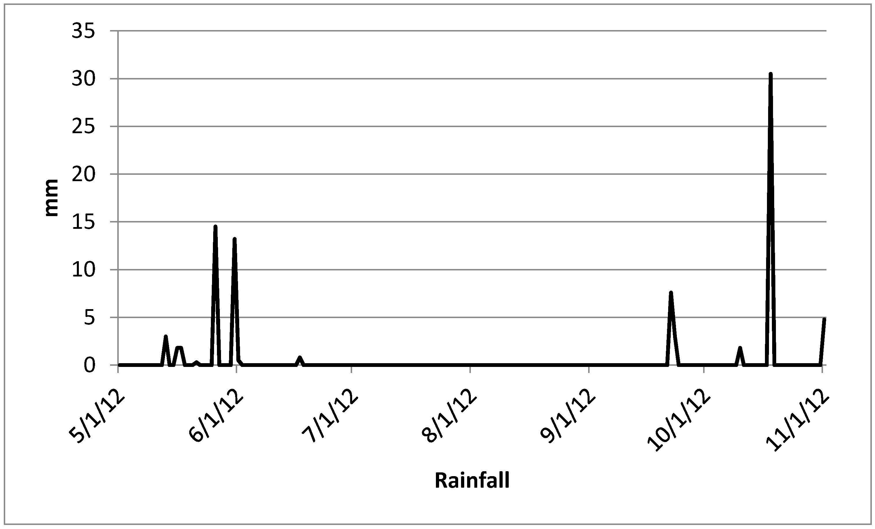
2.1. Study Area
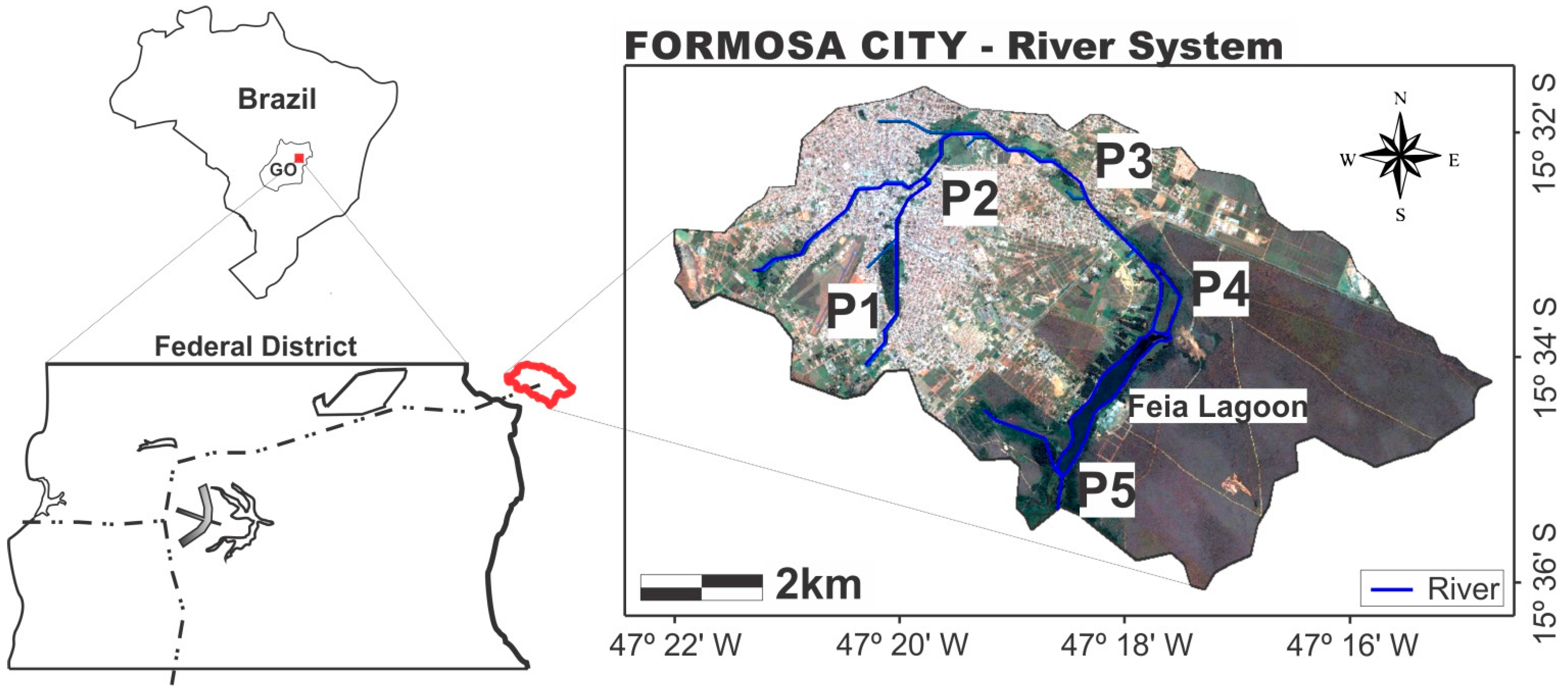
2.2. Analytical Methodologies
2.3. Statistical Analysis
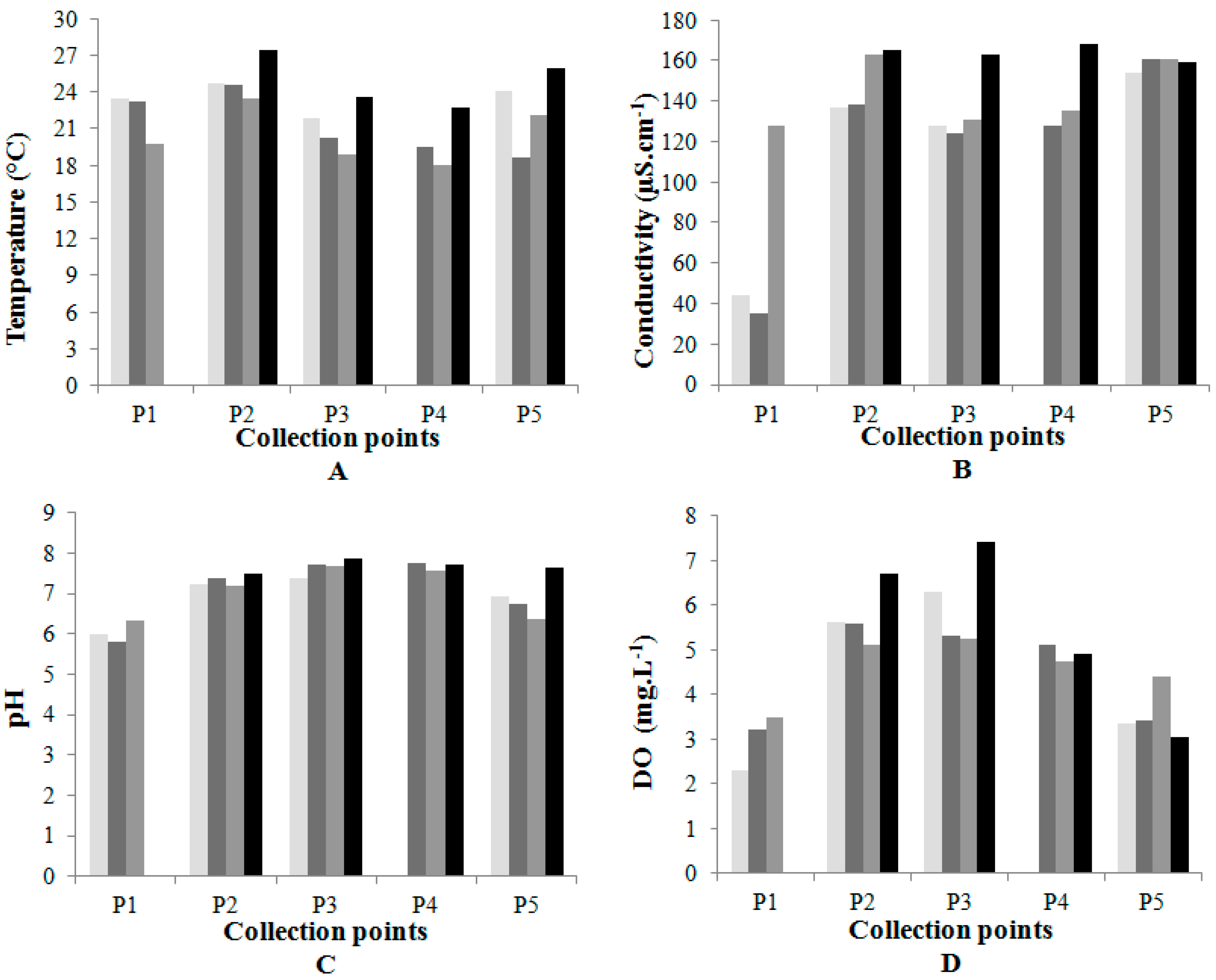
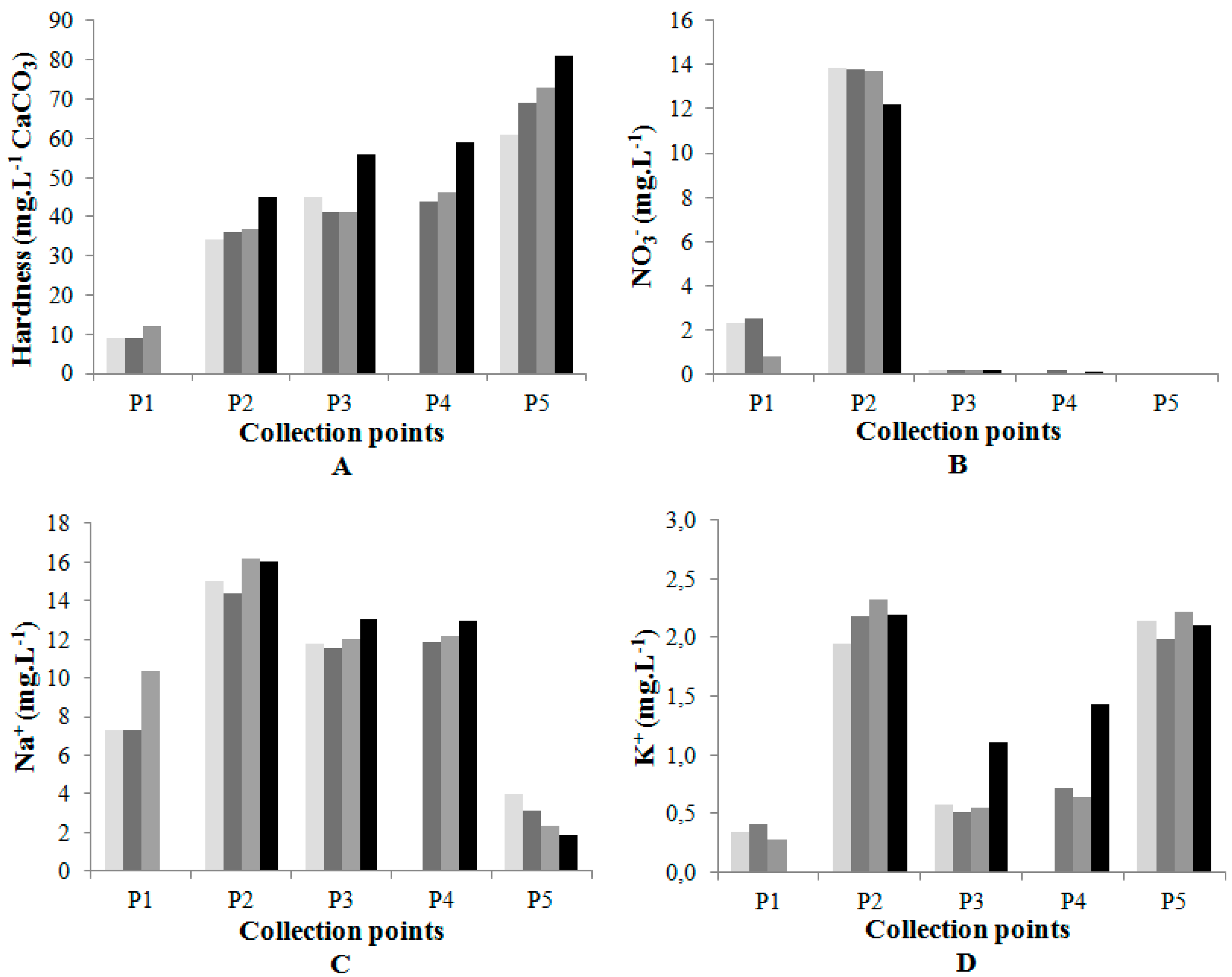
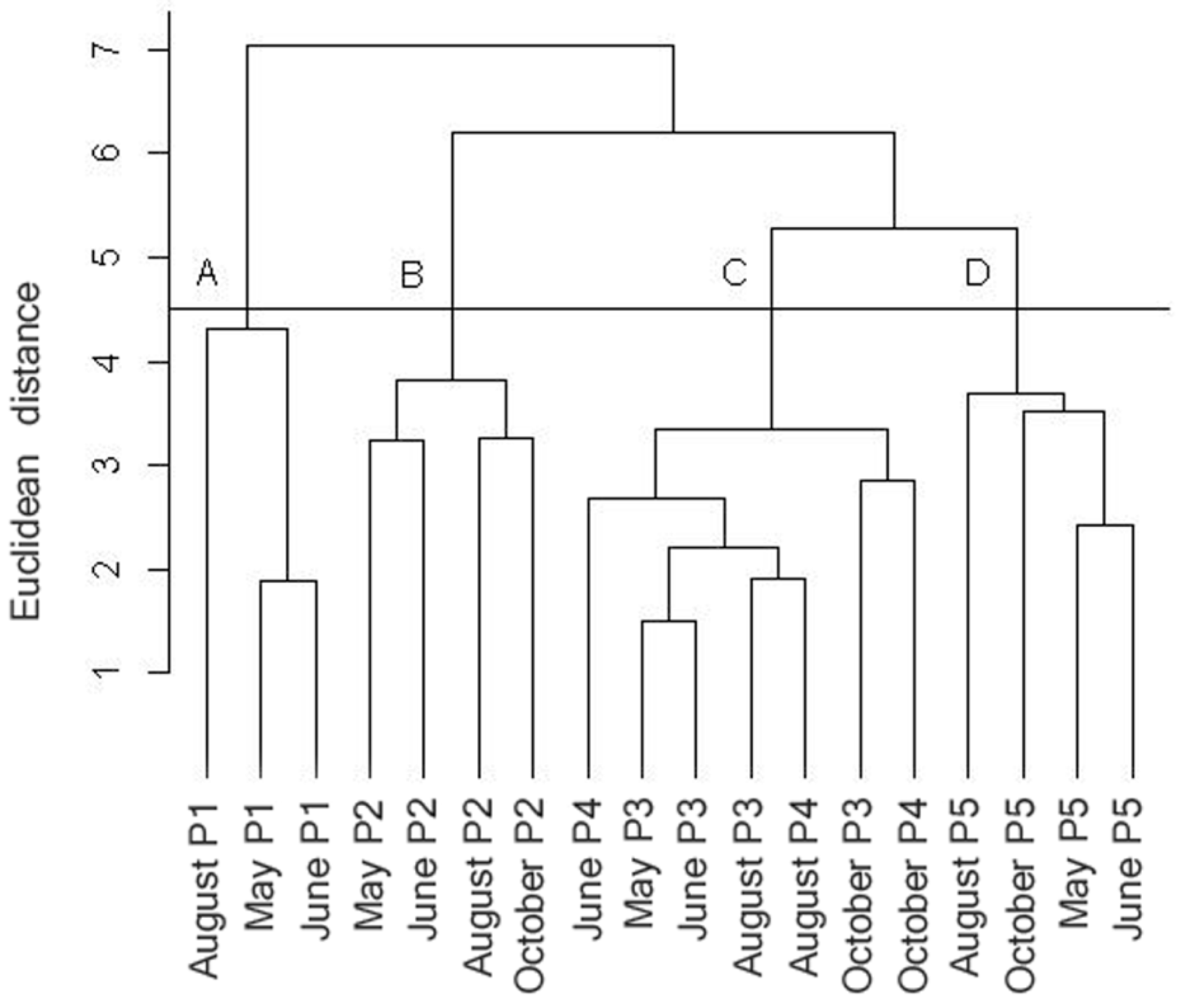
3. Results and Discussion
3.1. Physical-Chemical and Biological Analyses

| Collection Points | Temp. (*) (°C) | EC (µS·cm−1) | TDS (mg·L−1) | Turbidity (NTU) | pH | DO (mg·L−1) | Hardness (mg·L−1 CaCO3) |
|---|---|---|---|---|---|---|---|
| Collection date: May 07 | |||||||
| P1 | 23.5 | 44 | 22 | 0.11 | 5.9 | 2.3 | 9 |
| P2 | 24.7 | 137 | 68 | 0.78 | 7.2 | 5.6 | 34 |
| P3 | 21.9 | 128 | 64 | 1.18 | 7.4 | 6.3 | 45 |
| P4 | (**) | (**) | (**) | (**) | (**) | (**) | (**) |
| P5 | 24.1 | 154 | 77 | 0.02 | 6.9 | 3.3 | 61 |
| Collection date: June 25 | |||||||
| P1 | 23.2 | 35 | 18 | 2.29 | 5.8 | 3.2 | 9 |
| P2 | 24.1 | 138 | 69 | 5.29 | 7.4 | 5.6 | 36 |
| P3 | 20.2 | 124 | 62 | 1.86 | 7.7 | 5.3 | 41 |
| P4 | 19.5 | 128 | 64 | 4.94 | 7.7 | 5.1 | 44 |
| P5 | 18.7 | 161 | 81 | 1.43 | 6.7 | 3.4 | 69 |
| Collection date: August 13 | |||||||
| P1 | 19.7 | 128 | 64 | 2.52 | 6.3 | 3.5 | 12 |
| P2 | 23.5 | 163 | 82 | 3.98 | 7.2 | 5.1 | 37 |
| P3 | 18.8 | 131 | 65 | 2.12 | 7.2 | 5.3 | 41 |
| P4 | 18.1 | 135 | 68 | 3.08 | 7.6 | 4.7 | 46 |
| P5 | 22.1 | 161 | 81 | 3.72 | 6.4 | 4.4 | 73 |
| Collection date: October 01 | |||||||
| P1 | (***) | (***) | (***) | (***) | (***) | (***) | (***) |
| P2 | 27.4 | 165 | 83 | 1.95 | 7.5 | 6.7 | 45 |
| P3 | 23.6 | 163 | 81 | 5.12 | 7.8 | 7.4 | 56 |
| P4 | 22.8 | 168 | 84 | 1.88 | 7.7 | 4.9 | 59 |
| P5 | 25.9 | 159 | 79 | 3.24 | 7.6 | 3.1 | 81 |
| Points | F− (mg·L−1) | Cl− (mg·L−1) | NO2− (mg·L−1) | NO3− (mg·L−1) | SO42− (mg·L−1) | Na+ (mg·L−1) | K+ (mg·L−1) | Ca+ (mg·L−1) | Mg+ (mg·L−1) |
|---|---|---|---|---|---|---|---|---|---|
| Collection date: May 07 | |||||||||
| P1 | 0.04 | 2.43 | n.d. | 2.28 | 0.30 | 7.32 | 0.34 | 4.01 | 0.40 |
| P2 | 0.05 | 7.03 | 0.06 | 13.85 | 0.90 | 15.03 | 1.95 | 8.50 | 1.22 |
| P3 | 0.05 | 4.06 | n.d. | 0.17 | 0.48 | 11.76 | 0.57 | 8.46 | 1.38 |
| P4 | (*) | (*) | (*) | (*) | (*) | (*) | (*) | (*) | (*) |
| P5 | 0.03 | 1.58 | n.d. | n.d. | 0.45 | 4.01 | 2.14 | 12.28 | 4.63 |
| Collection date: June 25 | |||||||||
| P1 | 0.05 | 2.75 | n.d. | 2.53 | 0.57 | 7.26 | 0.41 | 4.59 | 0.45 |
| P2 | 0.09 | 7.59 | 0.10 | 13.81 | 1.13 | 14.38 | 2.19 | 8.51 | 1.40 |
| P3 | 0.07 | 4.95 | n.d. | 0.16 | 0.67 | 11.53 | 0.51 | 9.05 | 1.42 |
| P4 | 0.02 | 4.99 | n.d. | 0.15 | 0.74 | 11.84 | 0.72 | 9.79 | 1.55 |
| P5 | 0.01 | 1.27 | n.d. | n.d. | 0.35 | 3.11 | 1.99 | 10.37 | 5.65 |
| Collection date: August 13 | |||||||||
| P1 | 0.06 | 5.05 | n.d. | 0.77 | 0.66 | 10.36 | 0.28 | 3.50 | 0.33 |
| P2 | 0.11 | 8.72 | 0.09 | 13.69 | 3.80 | 16.21 | 2.33 | 10.43 | 1.40 |
| P3 | 0.03 | 5.09 | n.d. | 0.19 | 0.56 | 11.99 | 0.55 | 13.26 | 1.35 |
| P4 | 0.08 | 5.49 | n.d. | n.d. | 0.63 | 12.17 | 0.64 | 14.53 | 1.61 |
| P5 | 0.09 | 1.19 | n.d. | n.d. | 0.40 | 2.34 | 2.22 | 15.98 | 6.28 |
| Collection date: October 01 | |||||||||
| P1 | (**) | (**) | (**) | (**) | (**) | (**) | (**) | (**) | (**) |
| P2 | 0.11 | 8.62 | 0.24 | 12.17 | 2.10 | 16.06 | 2.20 | 14.05 | 1.77 |
| P3 | 0.04 | 5.88 | n.d. | 0.15 | 0.34 | 13.01 | 1.10 | 15.52 | 1.86 |
| P4 | 0.05 | 5.98 | n.d. | 0.08 | 0.46 | 12.92 | 1.43 | 15.71 | 1.98 |
| P5 | 0.02 | 0.65 | n.d. | n.d | 0.07 | 1.89 | 2.11 | 12.79 | 7.10 |
| Date | P1 | P2 | P3 | P4 | P5 |
|---|---|---|---|---|---|
| Total coliforms (NMP/100 mL) | |||||
| 07/05/2012 | 1732.9 | >2419.6 | >2419.6 | (*) | >2419.6 |
| 25/06/2012 | 1299.7 | >2419.6 | >2419.6 | >2419.6 | >2419.6 |
| 13/08/2012 | 920.8 | >2419.6 | >2419.6 | >2419.6 | >2419.6 |
| 01/10/2012 | (**) | >2419.6 | >2419.6 | >2419.6 | 1732.9 |
| Thermotolerant coliforms (NMP/100 mL) | |||||
| 07/05/2012 | 307.6 | >2419.6 | 248.1 | (*) | 33.1 |
| 25/06/2012 | 98.4 | >2419.6 | 648.8 | 727.0 | 18.7 |
| 13/08/2012 | 261.3 | 1986.3 | 365.4 | 770.1 | 290.9 |
| 01/10/2012 | (**) | >2419.6 | 613.1 | 166.4 | 107.1 |
3.2. Statistical Analysis
| Variables | Mean | Standard Deviation | Minimum | Maximum |
|---|---|---|---|---|
| Water Temperature | 22.35 | 2.66 | 18.08 | 27.40 |
| pH | 7.15 | 0.64 | 5.81 | 7.85 |
| Conductivity | 134.6 | 37.90 | 35.00 | 168.00 |
| TDS | 67.32 | 18.92 | 18.00 | 84.00 |
| DO | 4.73 | 1.38 | 2.29 | 7.42 |
| Hardness | 44.32 | 20.58 | 9.00 | 81.00 |
| Turbidity | 2.52 | 1.61 | 0.02 | 5.29 |
| Coliforms | 2197.81 | 457.51 | 920.80 | 2419.60 |
| E.coli | 772.28 | 880.66 | 18.70 | 2419.60 |
| Sodium | 10.17 | 4.71 | 1.89 | 16.21 |
| Potassium | 1.31 | 0.28 | 0.34 | 2.33 |
| Calcium | 10.63 | 3.50 | 4.01 | 15.98 |
| Magnesium | 2.32 | 0.33 | 0.40 | 7.10 |
| Fluoride | 0.06 | 0.01 | 0.02 | 0.11 |
| Chloride | 4.63 | 2.53 | 0.66 | 8.72 |
| Nitrite | 0.03 | 0.06 | 0.00 | 0.24 |
| Nitrate | 3.33 | 5.58 | 0.00 | 13.85 |
| Sulfate | 0.82 | 0.85 | 0.30 | 3.80 |
| Summary Anova | ||
|---|---|---|
| Variables | F Value | p Value |
| Water Temperature | 4.116 | 0.0275 * |
| pH | 1.238 | 0.333 |
| Conductivity | 1.779 | 0.197 |
| TDS | 1.766 | 0.2 |
| DO | 0.52 | 0.675 |
| Hardness | 1.075 | 0.391 |
| Turbidity | 4.129 | 0.0272 * |
| E.coli | 0.007 | 0.999 |
| Sodium | 0.084 | 0.968 |
| Potassium | 0.374 | 0.773 |
| Calcium | 3.234 | 0.0547 |
| Fluoride | 1.071 | 0.393 |
| Chloride | 0.287 | 0.834 |
| Summary Anova | ||
|---|---|---|
| Variables | F Value | p Value |
| Water Temperature | 2.353 | 0.108 |
| pH | 16.39 | 5.37E-05 * |
| Conductivity | 6.831 | 0.00345 * |
| TDS | 6.841 | 0.00342 * |
| DO | 13.41 | 0.000152 * |
| Hardness | 38 | 4.69E-07 * |
| Turbidity | 0.489 | 0.744 |
| E.coli | 74.46 | 7.91E-09 * |
| Sodium | 90.64 | 2.33E-09 * |
| Potassium | 46.31 | 1.44E-07 * |
| Calcium | 6.263 | 0.00491 * |
| Fluoride | 2.214 | 0.124 |
| Chloride | 37.32 | 5.22E-07 * |
4. Conclusions
Acknowledgements
Author Contributions
Conflicts of Interest
References
- Von Sperling, M. Introdução à Qualidade das Águas e ao Tratamento de Esgotos, 1st ed.; Editora UFMG: Belo Horizonte, Brasil, 2005. (In Portuguese) [Google Scholar]
- Lima, J.E.F.W. Recursos Hídricos no Brasil e no Mundo, 1st ed.; Embrapa Cerrados: Planaltina-DF, Brasil, 2001. (In Portuguese) [Google Scholar]
- Lima, J.E.F.W.; Silva, E.M. Recursos hídricos do Bioma Cerrado. In Cerrado: Ecologia e Flora; Sano, S.M., Ribeiro, J.F., Eds.; Embrapa Cerrados: Brasília, Brasil, 2008; Volume 1, p. 46. (In Portuguese) [Google Scholar]
- Oliveira-Filho, E.C.; Medeiros, F.N.S. Ocupação humana e preservação do ambiente: Um paradoxo para o desenvolvimento sustentável. In Cerrado: Desafios e Oportunidades Para o Desenvolvimento Sustentável; Embrapa Cerrados: Brasília, Brasil, 2008; Volume 1, pp. 33–61. (In Portuguese) [Google Scholar]
- Muniz, D.H.F.; Moraes, A.S.; Freire, I.S.; Cruz, C.J.D.; Lima, J.E.F.W.; Oliveira-Filho, E.C. Evaluation of water quality parameters for monitoring natural, urban, and agricultural areas in the Brazilian Cerrado. Acta Limnol. Bras. 2011, 3, 307–317. [Google Scholar] [CrossRef]
- Chauvet, G. Brasília e Formosa: 4.500 anos de história, 1st ed.; Kelps: Goiânia, Brasil, 2005. [Google Scholar]
- SEPIN. Superintendência de Estatística, Pesquisa e Informações Socioeconômicas: Formosa. http://www.seplan.go.gov.br/sepin/ (accessed on 22 May 2015).
- Associação Brasileira de Normas Técnicas. Água: Determinação da Dureza Total—Método Titulométrico do EDTA-NA Método de Ensaio; NBR 12621; ABNT: Rio de Janeiro, Brasil, 1992. (In Portuguese) [Google Scholar]
- Association, Standard Methods for Examination of Water and Wastewater, 20th ed.; APHA: Washington, DC, USA, 1998.
- Durbin, J. Distribution Theory for Test Based on the Sample Distribution Function, 5th ed.; Siam: London, UK, 2004. [Google Scholar]
- Marsaglia, G.; Tsang, W.W.; Wang, J. Evaluating Kolmogorov’s distribution. J. Stat. Softw. 2003, 8, 1–4. [Google Scholar]
- Chambers, J.M.; Freeny, A.; Heiberger, R.M. Analysis of variance; designed experiments. In Statistical Models; Chambers, J.M., Hastie, T.S., Eds.; Wadsworth & Brooks/Cole: Pacific Grove, Ca, USA, 1992. [Google Scholar]
- Winter, T.C.; Harvey, J.W.; Franke, O.L.; Alley, W.M. Ground Water and Surface Water: A Single Resource; U.S. Government Printing Office: Denver, CO, USA, 1998. [Google Scholar]
- Bocard, D.; Gillet, F.; Legendre, P. Numerical Ecology with R; Springer: New York, NY, USA, 2011. [Google Scholar]
- Legendre, P.; Legendre, L.F.J. Numerical Ecology; Elsevier: Amsterdam, Netherlands, 2012. [Google Scholar]
- CETESB. Companhia de Tecnologia de Saneamento Ambiental. In Relatório de Qualidade das Águas Interiores do Estado de São Paulo 2003, 1st ed.; Série relatórios: São Paulo, Brasil, 2004. [Google Scholar]
- Oliveira-Filho, E.C.; Caixeta, N.R.; Simplício, N.C.S.; Sousa, S.R.; Aragão, T.P.; Muniz, D.H.F. Implications of water hardness in ecotoxicological assessments for water quality regulatory purposes: A case study with the aquatic snail Biomphalaria glabrata. Braz. J. Biol. 2014, 1, 175–180. [Google Scholar] [CrossRef]
- Jacobson, T.K.B.; Bustamante, M.M.C.; Kozovits, A.R. Diversity of shrub tree layer, leaf litter decomposition and N release in a Brazilian Cerrado under N, P and N plus P additions. Environ. Pollut. 2011, 159, 2236–2242. [Google Scholar] [CrossRef] [PubMed]
- Meyer, W.M., III; Ostertag, R.; Cowie, R.W. Macro-invertebrates accelerate litter decomposition and nutrient release in an Hawaiian rainforest. Soil Biol. Biochem. 2011, 43, 206–211. [Google Scholar] [CrossRef]
- Souza, A.L.T.; Fonseca, D.G.; Libório, R.A.; Tanaka, M.O. Influence of riparian vegetation and forest structure on the water quality of rural low-order streams in SE Brazil. For. Ecol. Manag. 2013, 298, 12–18. [Google Scholar] [CrossRef]
- Brasil. Vigilância e Controle da Qualidade da Água Para Consumo Humano, 1st ed.; Ministério da Saúde: Brasília, Brasil, 2006. (In Portuguese) [Google Scholar]
- Neves, T.; Foloni, L.L.; Pitelli, R.A. Chemical control of waterhyacinth (Eichhornia crassipes). Planta Daninha 2002, 20, 89–97. (In Portuguese) [Google Scholar] [CrossRef]
- Martins, A.P.L.; Reissmann, C.B.; Favareto, N.; Boeger, M.R.T.; Oliveira, E.B. Capacidade de Typha dominguensis na fitorremediação de efluentes de tanques de piscicultura na Bacia do Iraí. Rev. Bras. Eng. Agric. Ambient. 2007, 11, 324–330. (In Portuguese) [Google Scholar] [CrossRef]
- Tucci, C.E.M. Hidrologia: Ciências e aplicação, 4th ed.; UFRGS: Porto Alegre, Brasil, 2007; pp. 806–809. (In Portuguese) [Google Scholar]
- Gasparino, D.; Malavasi, U.C.; Malavasi, M.M.; Souza, I. Quantificação do banco de sementes sob diferentes usos do solo em área de domínio ciliar. Rev. Árvore 2006, 30, 1–9. (In Portuguese) [Google Scholar] [CrossRef]
- Lima, I.L.P.; Scariot, A.; Medeiros, M.B.; Sevilha, A.C. Diversidade e uso de plantas do Cerrado em comunidade de Geraizeiros no norte do estado de Minas Gerais, Brasil. Acta Bot. Bras. 2012, 26, 675–684. (In Portuguese) [Google Scholar] [CrossRef]
- Cabral, J.P.S. Water microbiology. Bacterial pathogens and water. Int. J. Environ. Res. Public Health 2010, 7, 3657–3703. [Google Scholar] [CrossRef] [PubMed]
© 2015 by the authors; licensee MDPI, Basel, Switzerland. This article is an open access article distributed under the terms and conditions of the Creative Commons Attribution license (http://creativecommons.org/licenses/by/4.0/).
Share and Cite
Pires, N.L.; Muniz, D.H.d.F.; Kisaka, T.B.; Simplicio, N.D.C.S.; Bortoluzzi, L.; Lima, J.E.F.W.; Oliveira-Filho, E.C. Impacts of the Urbanization Process on Water Quality of Brazilian Savanna Rivers: The Case of Preto River in Formosa, Goiás State, Brazil. Int. J. Environ. Res. Public Health 2015, 12, 10671-10686. https://doi.org/10.3390/ijerph120910671
Pires NL, Muniz DHdF, Kisaka TB, Simplicio NDCS, Bortoluzzi L, Lima JEFW, Oliveira-Filho EC. Impacts of the Urbanization Process on Water Quality of Brazilian Savanna Rivers: The Case of Preto River in Formosa, Goiás State, Brazil. International Journal of Environmental Research and Public Health. 2015; 12(9):10671-10686. https://doi.org/10.3390/ijerph120910671
Chicago/Turabian StylePires, Nayara Luiz, Daphne Heloisa de Freitas Muniz, Tiago Borges Kisaka, Nathan De Castro Soares Simplicio, Lilian Bortoluzzi, Jorge Enoch Furquim Werneck Lima, and Eduardo Cyrino Oliveira-Filho. 2015. "Impacts of the Urbanization Process on Water Quality of Brazilian Savanna Rivers: The Case of Preto River in Formosa, Goiás State, Brazil" International Journal of Environmental Research and Public Health 12, no. 9: 10671-10686. https://doi.org/10.3390/ijerph120910671
APA StylePires, N. L., Muniz, D. H. d. F., Kisaka, T. B., Simplicio, N. D. C. S., Bortoluzzi, L., Lima, J. E. F. W., & Oliveira-Filho, E. C. (2015). Impacts of the Urbanization Process on Water Quality of Brazilian Savanna Rivers: The Case of Preto River in Formosa, Goiás State, Brazil. International Journal of Environmental Research and Public Health, 12(9), 10671-10686. https://doi.org/10.3390/ijerph120910671