
Spatial and Temporal Distribution of PM2.5 Pollution in Xi’an City, China

Abstract
:1. Introduction
- The distribution features of PM2.5, on the scale of time and space; and
- The influential distribution factors, from the prospects of human activity and metrological factors.
2. Materials and Methods
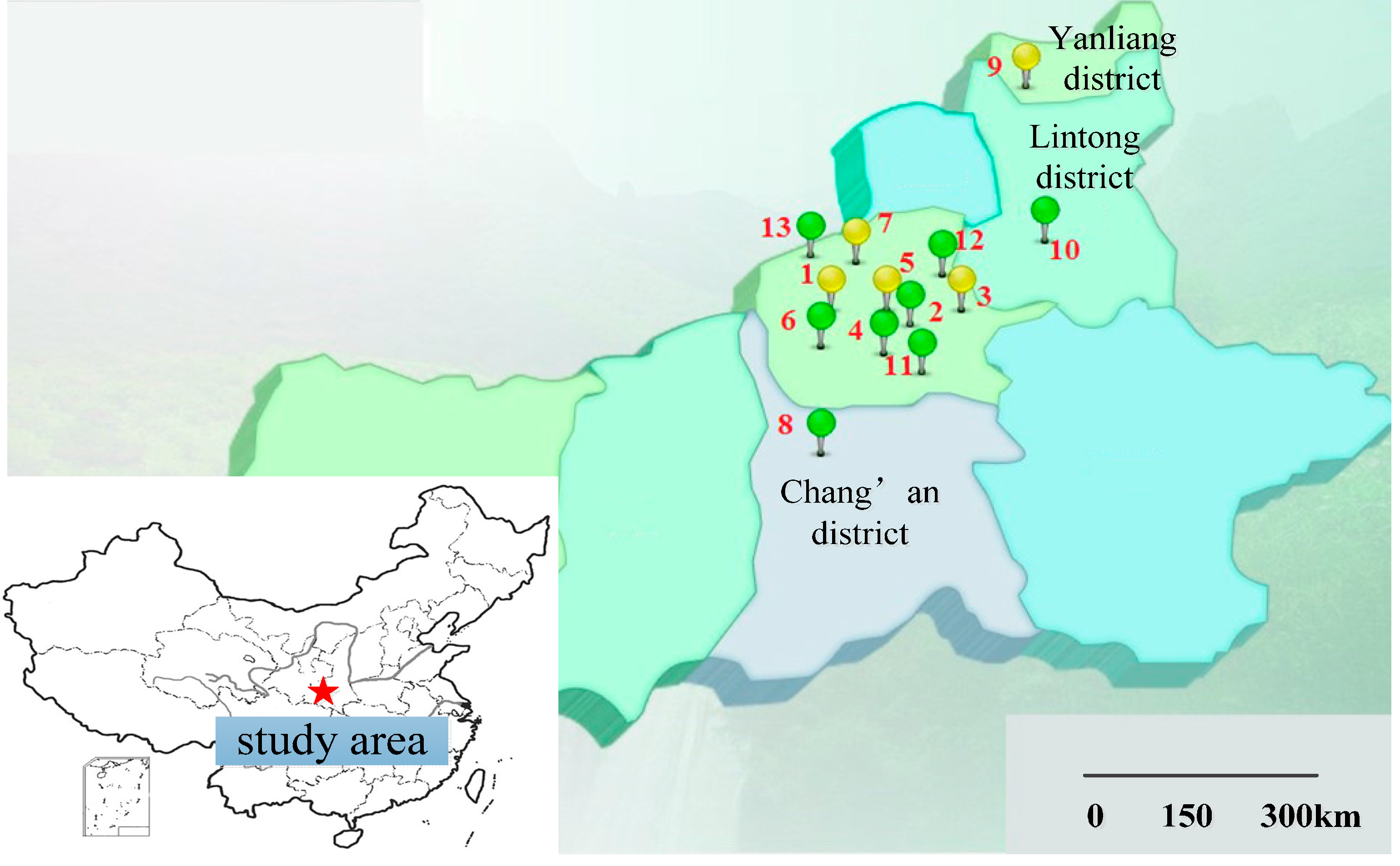
2.1. Data

| Number | Monitoring Sites | Samples | Maximum | Minimum | ρ(PM2.5)/(μg/m3) | ||||||
|---|---|---|---|---|---|---|---|---|---|---|---|
| Mean | Standard Deviation | ||||||||||
| 2013 | 2014 | 2013 | 2014 | 2013 | 2014 | 2013 | 2014 | 2013 | 2014 | ||
| 1 | High-voltage Switch Factory | 365 | 365 | 500 | 500 | 18 | 15 | 144.752 | 108.156 | 107.074 | 71.822 |
| 2 | Xingqing district | 365 | 365 | 500 | 500 | 13 | 10 | 112.621 | 103.942 | 105.785 | 85.320 |
| 3 | Textile city | 365 | 365 | 496 | 470 | 15 | 13 | 129.704 | 106.948 | 94.877 | 68.811 |
| 4 | Xiaozhai | 365 | 365 | 500 | 496 | 10 | 10 | 125.724 | 97.426 | 98.628 | 70.467 |
| 5 | People’s Stadium | 365 | 365 | 500 | 500 | 18 | 20 | 152.915 | 114.319 | 109.554 | 80.374 |
| 6 | High-tech Western | 365 | 365 | 500 | 500 | 15 | 5 | 142.112 | 99.873 | 106.453 | 79.108 |
| 7 | Economic development district | 365 | 365 | 474 | 500 | 16 | 15 | 131.985 | 102.775 | 96.902 | 72.520 |
| 8 | Chang’an district | 365 | 365 | 500 | 430 | 10 | 16 | 122.815 | 89.431 | 98.070 | 66.200 |
| 9 | Yanliang district | 365 | 365 | 452 | 484 | 15 | 16 | 127.734 | 94.181 | 92.069 | 65.968 |
| 10 | Lintong district | 365 | 365 | 500 | 500 | 13 | 15 | 136.406 | 98.365 | 102.559 | 72.012 |
| 11 | Qujiang cultural group | 365 | 365 | 500 | 376 | 3 | 12 | 114.521 | 95.695 | 94.720 | 64.349 |
| 12 | Guangyun Tan | 365 | 365 | 500 | 460 | 18 | 18 | 123.643 | 95.503 | 102.280 | 63.695 |
| 13 | Cao Tan | 365 | 365 | 500 | 500 | 12 | 12 | 163.705 | 111.151 | 107.575 | 80.394 |
2.2. Methodology
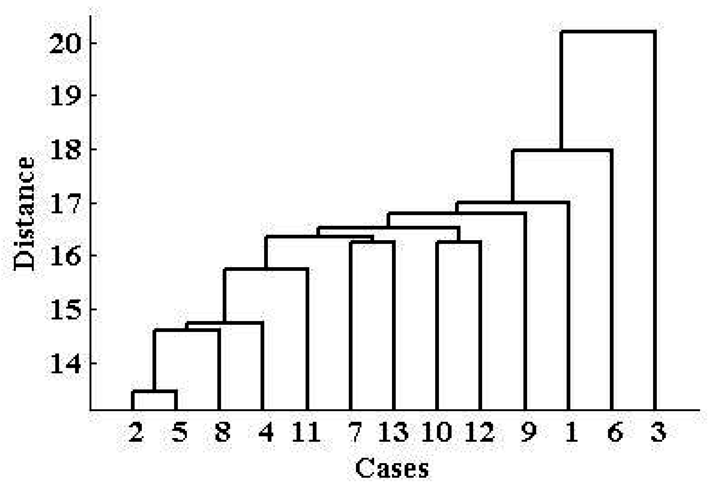
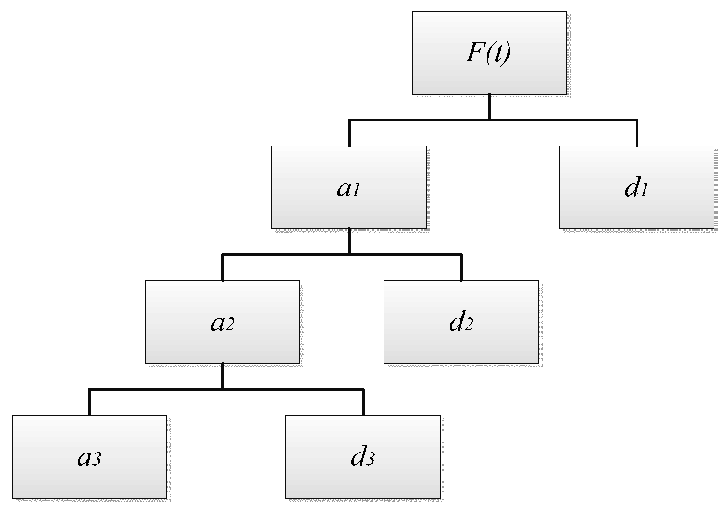
2.2.1. Cluster Analysis
- Step 1: Find the similarities and dissimilarities between different variables in the data set (the monitoring data of 13 sites in this paper), and calculate the distance (Euclidean distance in this paper) through the “pdist” function in MATLAB;
- Step 2: Define the linkage between different variables using the “linkage” function;
- Step 3: Assess the former calculation effect based on the “cophenetic” function;
- Step 4: Establish different clusters through the “cluster” function;
- Step 5: Obtain the hierarchial map through “plot”.
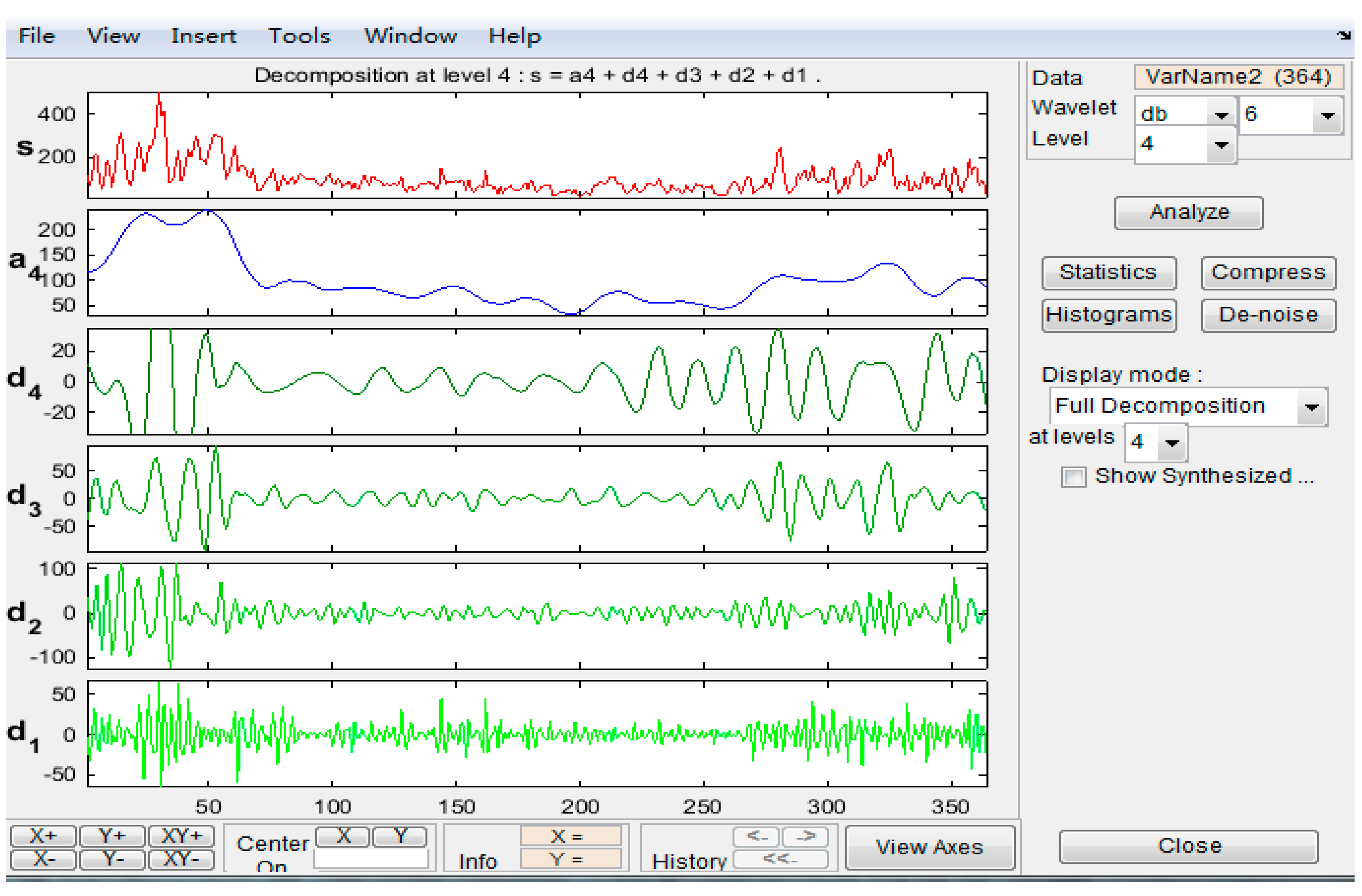
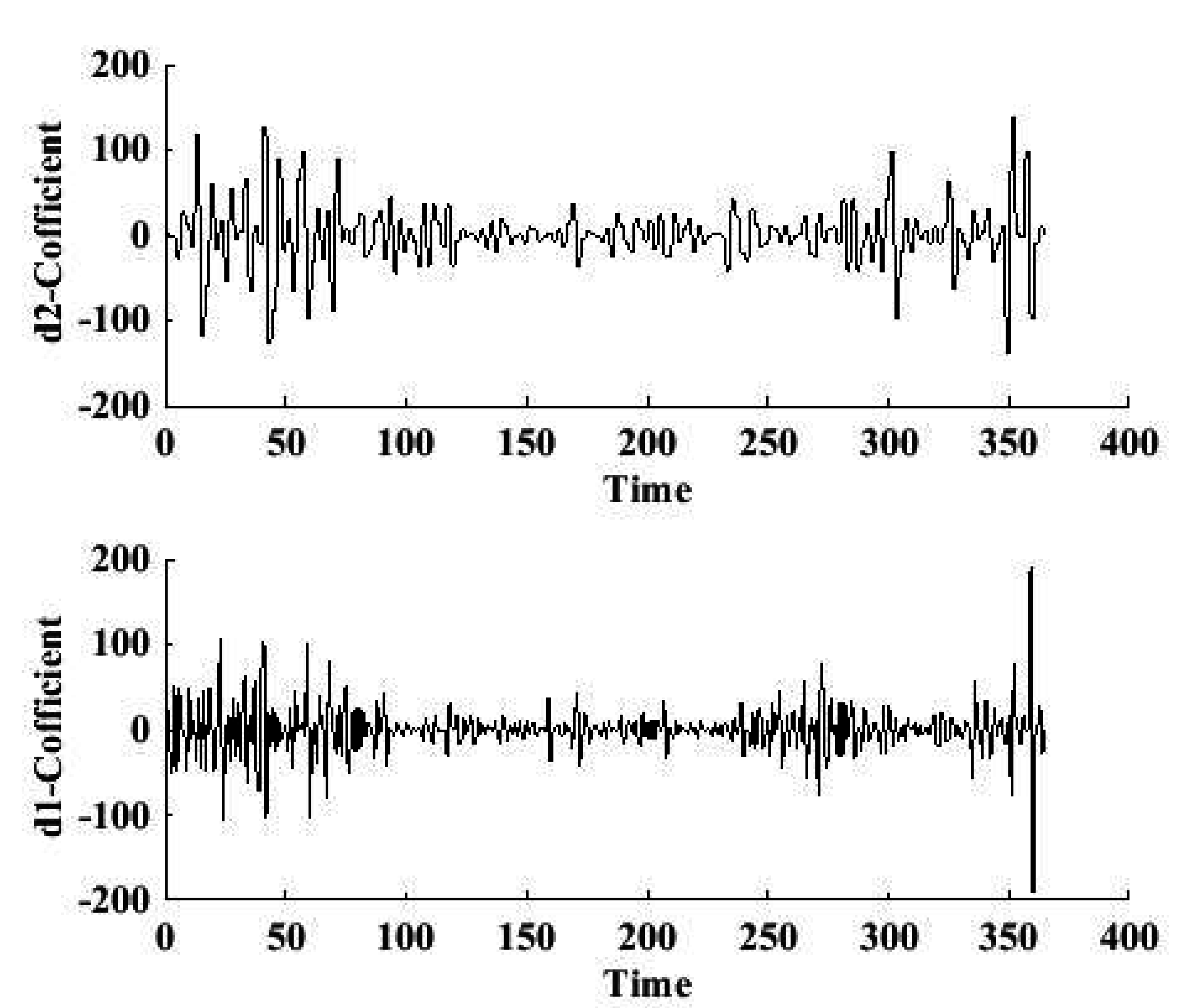
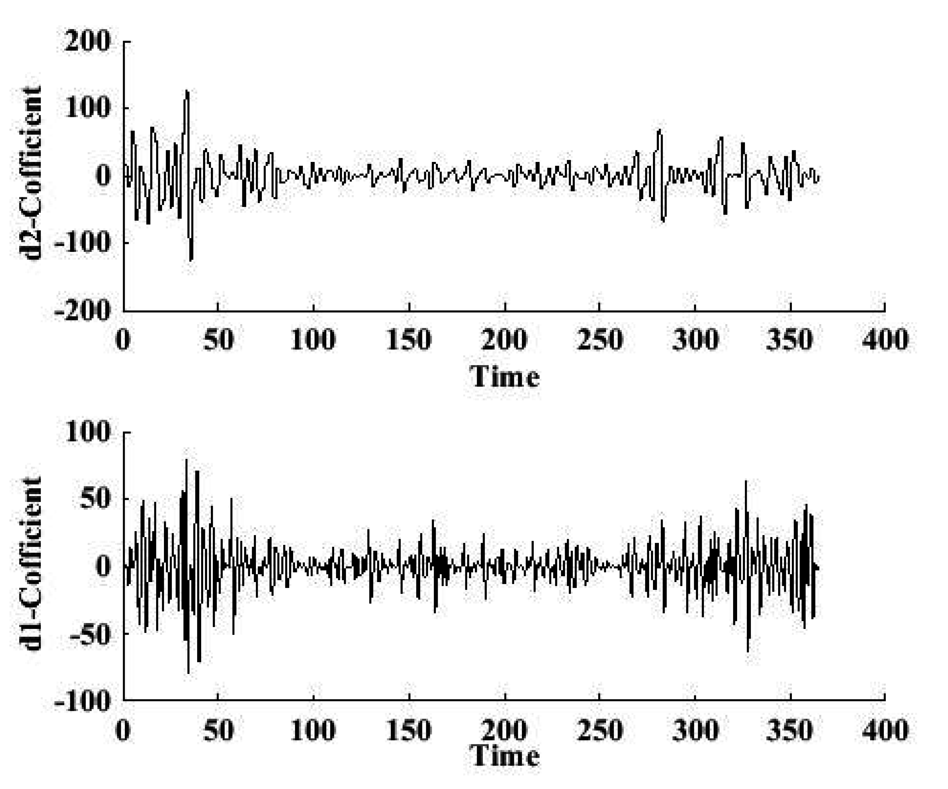
2.2.2. Wavelet Transform
3. Results and Discussions
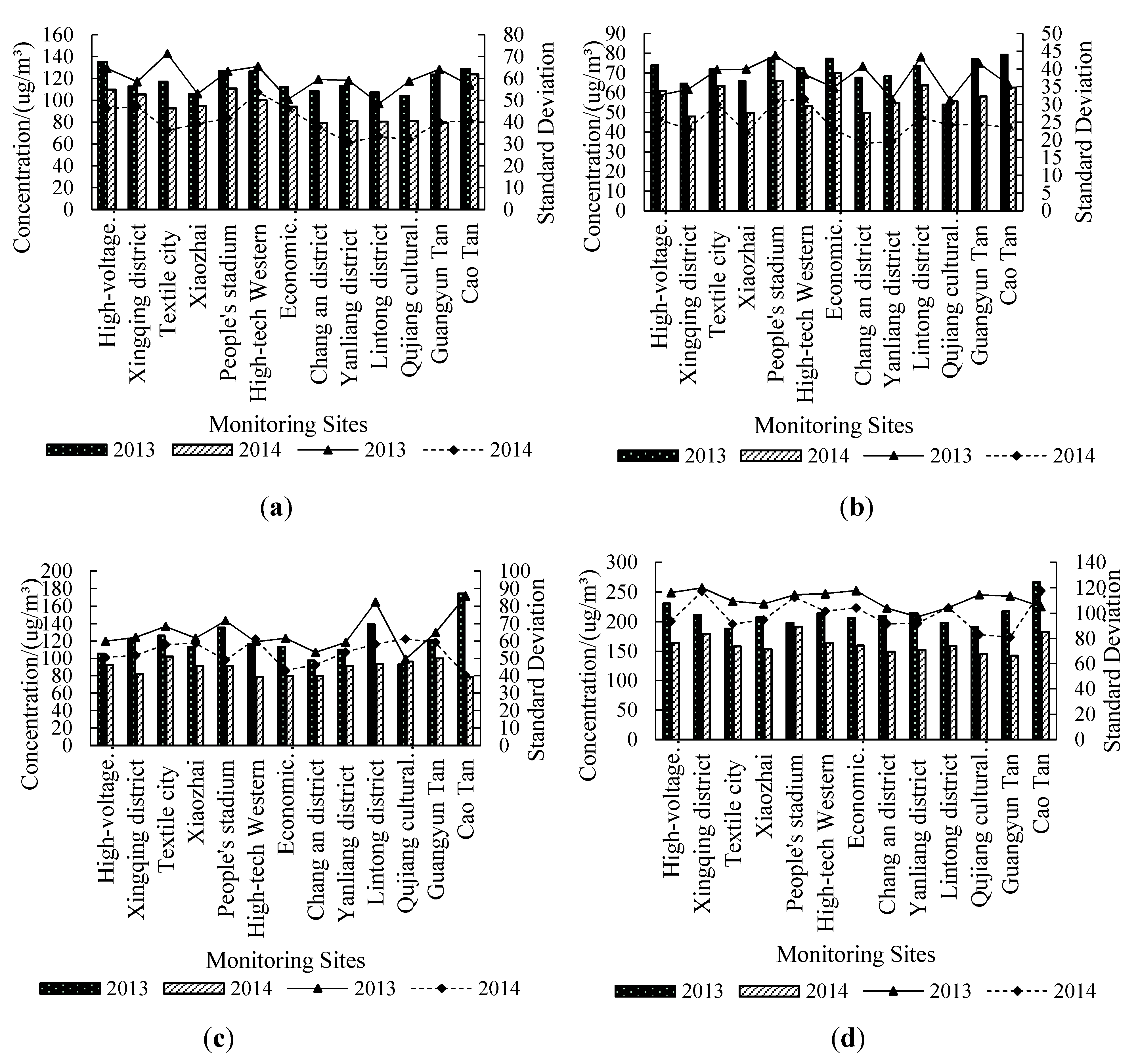
3.1. Distribution of ρ(PM2.5) in Time and Space


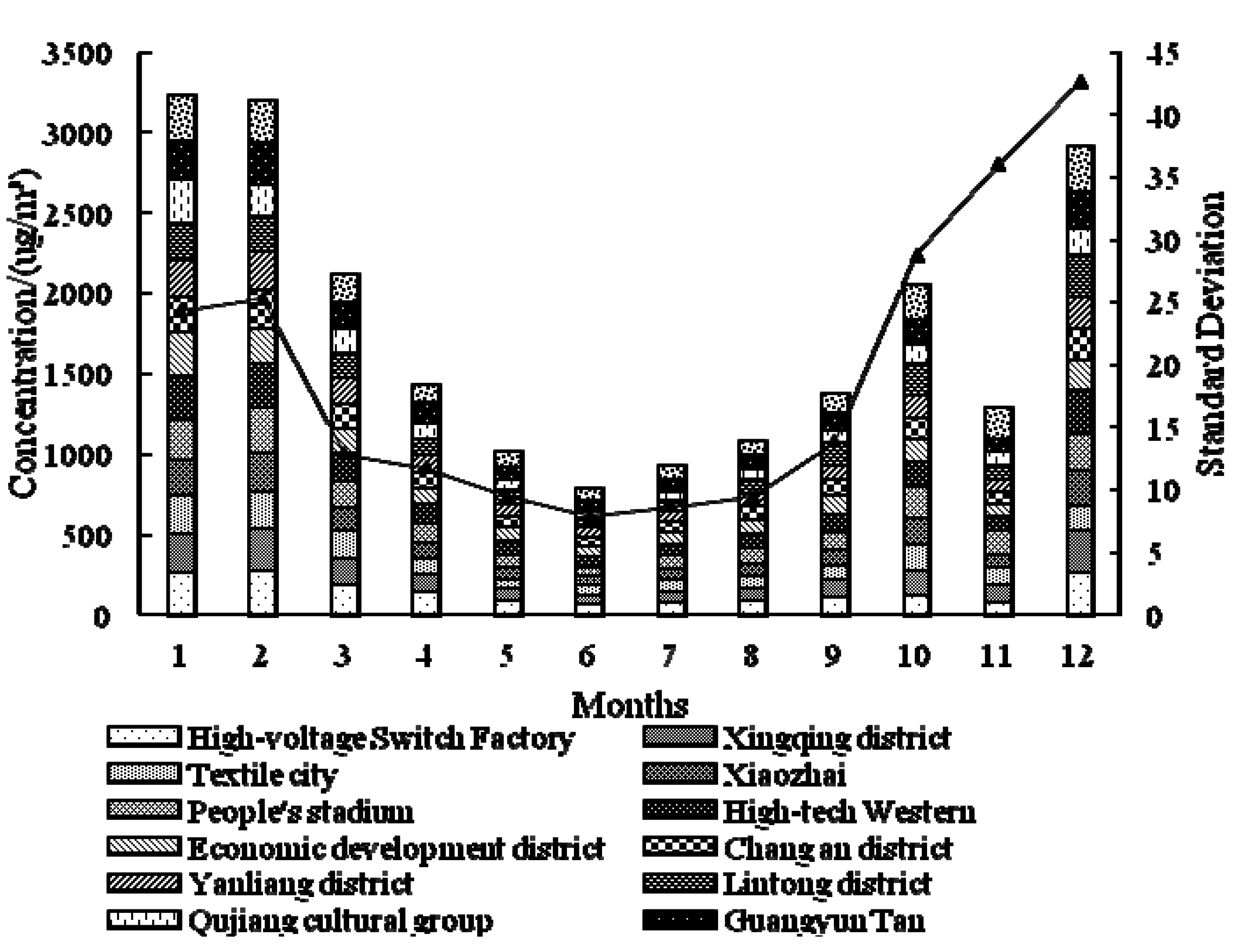

3.2. Regional Distribution Characteristic of ρ(PM2.5)

| Cluster | Sites | Main industrial Activities Characteristics |
|---|---|---|
| 1 | Textile city | Dense urban road networks, shopping malls and supermarkets dotted, textiles and clothing, aerospace technology, new materials, equipment manufacturing, modern service industry are the leading production |
| 2 | High-tech Western | Electrical machinery, refrigeration equipment, petroleum equipment, instrumentation |
| 3 | Xingqing district, Xiaozhai, People’s Stadium, Economic development district, Chang’an district, Yanliang dstrict, Lintong district, Qujiang cultural group, Guangyun Tan, and Cao Tan | Aluminum plant, profile plant, equipment factory, auto parts factory, aircraft industry, paper, flour, commercial vehicle industry, photovoltaic industry, agriculture, tourism |
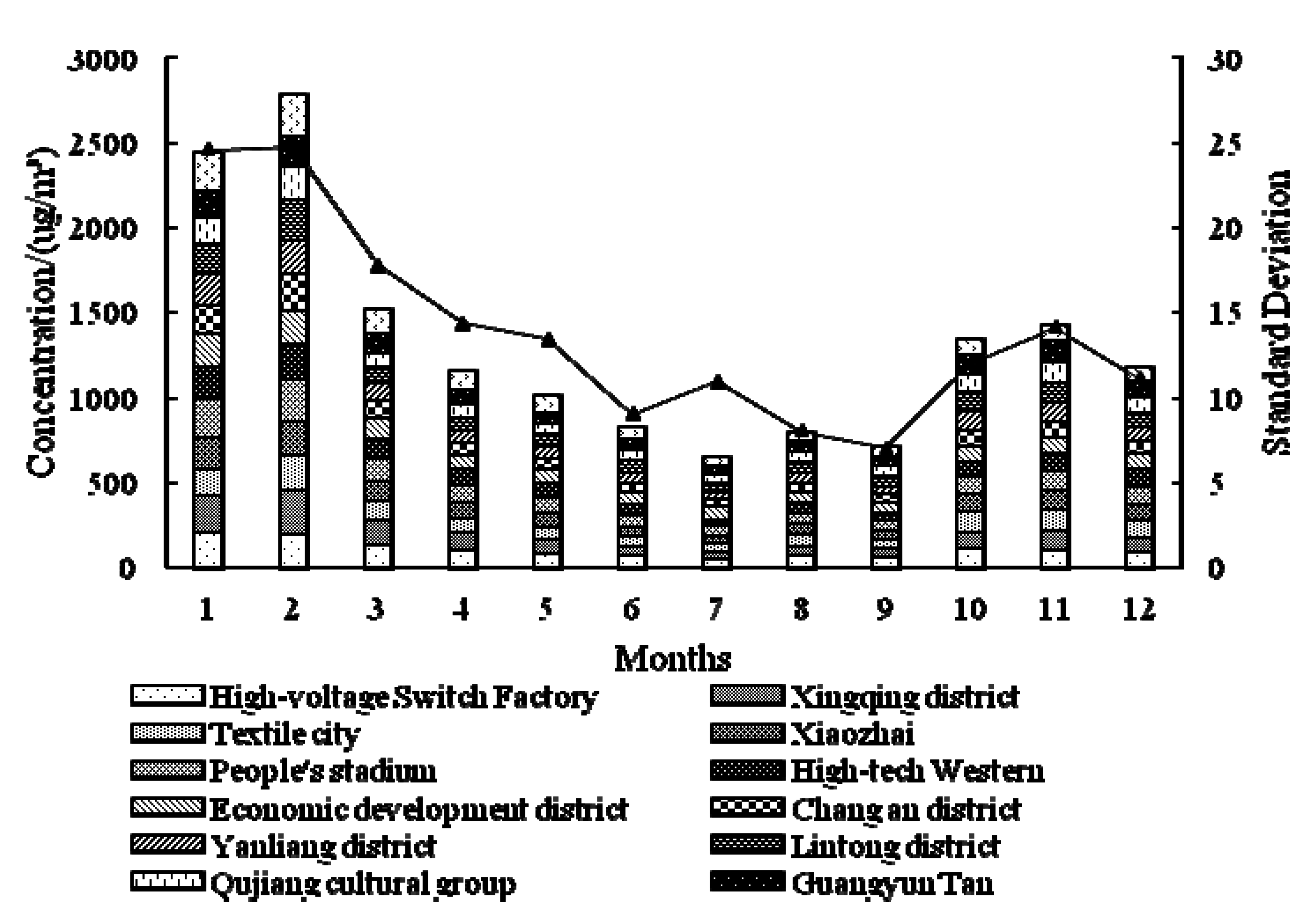
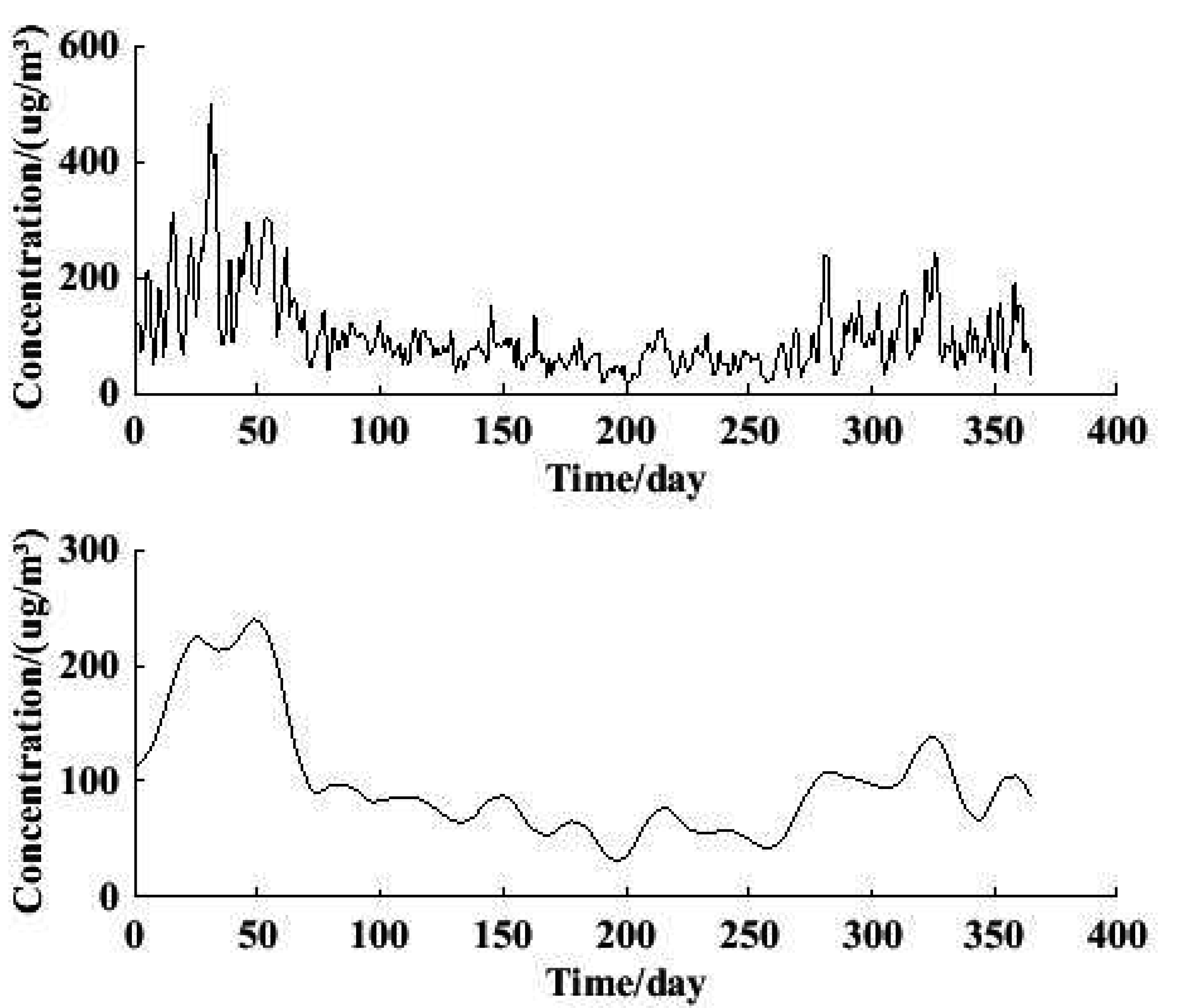
3.3. Time Series Analysis of PM2.5 Concentration
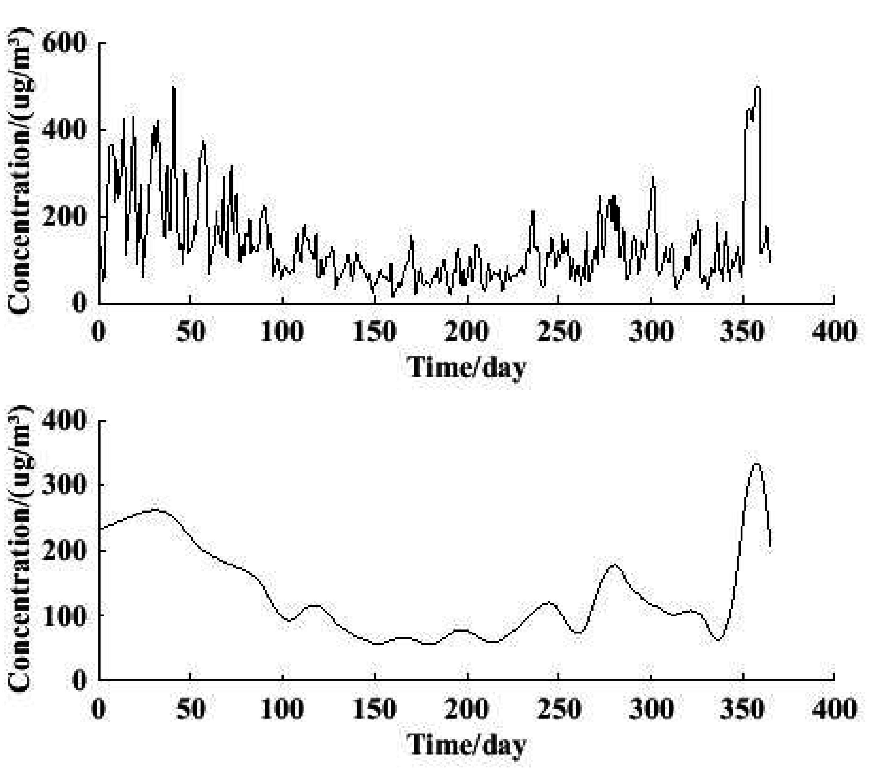


| Date(mm-dd) | ρ(PM2.5) (μg/m3) | Pollution Degree | Temperature/°C | Weather Condition | Wind Speed | |
|---|---|---|---|---|---|---|
| 2013 | 01-12 | 264 | Severe | −3–7 | Cloudy | <3 |
| 02-11 | 292 | Severe | −2–5 | Sleety | <3 | |
| 02-26 | 372 | Severe | 5–13 | Cloudy | <3 | |
| 03-12 | 260 | Severe | 7–16 | Cloudy | <3 | |
| 10-27 | 243 | Severe | 10–19 | Cloudy | <3 | |
| 12-17 | 278 | Severe | 9–12 | Hazy | <3 | |
| 12-24 | 500 | Severe | −2–3 | Hazy | <3 | |
| 2014 | 1-16 | 310 | Severe | −3–5 | Cloudy | <3 |
| 2-2 | 413 | Severe | 1–14 | Cloudy | <3 | |
3.4. Discussion
4. Conclusions
Supplementary Files
Supplementary File 1Acknowledgments
Author Contributions
Conflicts of Interest
References
- Han, L.; Zhou, W.; Li, W.; Li, L. Impact of urbanization level on urban air quality: A case of fine particles (PM2.5) in Chinese cities. Environ. Pollut. 2014, 194, 163–170. [Google Scholar] [CrossRef] [PubMed]
- Fu, M.; Martínez-Sánchez, J.M.; Galán, I.; Pérez-Ríos, M.; Sureda, X.; López, M.J.; Schiaffino, A.; Moncada, A.; Montes, A.; Nebot, M.; et al. Variability in the correlation between nicotine and PM2.5 as airborne markers of second-hand smoke exposure. Environ. Res. 2013, 127, 49–55. [Google Scholar] [CrossRef] [PubMed]
- Negral, L.; Moreno-Grau, S.; Moreno, J.; Querol, X.; Viana, M.M.; Alastuey, A. Natural and Anthropogenic Contributions to PM10 and PM2.5 in an Urban Area in the Western Mediterranean Coas. Water Air Soil Pollut. 2008, 192, 227–238. [Google Scholar] [CrossRef]
- Galea, K.S.; Hurley, J.F.; Cowie, H.; Shafrir, A.L.; Sánchez Jiménez, A.; Semple, S.; Ayres, J.G.; Coggins, M. Using PM2.5 concentrations to estimate the health burden from solid fuel combustion, with application to Irish and Scottish homes. Environ. Health 2013, 12, 50–52. [Google Scholar] [CrossRef] [PubMed]
- Shu, S.; Yang, P.; Zhu, Y. Correlation of noise levels and particulate matter concentrations near two major freeways in Los Angeles, California. Environ. Pollut. 2014, 193, 130–113. [Google Scholar] [CrossRef] [PubMed]
- Wang, J.; Zheng, J.; Ke, Z. Assessment of PM2.5 Exposure of residents in a community downwind of a typical industrial source. Res. Environ. Sci. 2012, 25, 745–750. [Google Scholar]
- Leung, P.Y.; Wan, H.T.; Billah, M.B.; Cao, J.J.; Ho, K.F.; Wong, C.K. Chemical and biological characterization of air particulate matter 2.5, collected from five cities in China. Environ. Pollut. 2014, 194, 188–195. [Google Scholar] [CrossRef] [PubMed]
- Langrish, J.P.; Li, X.; Wang, S.; Lee, M.M.; Barnes, G.D.; Miller, M.R.; Cassee, F.R.; Boon, N.A.; Donaldson, K.; Li, J.; et al. Reducing personal exposure to particulate air pollution improves cardiovascular health in patients with coronary heart disease. Environ. Health Perspect. 2012, 120, 367–372. [Google Scholar] [CrossRef] [PubMed]
- Rogge, W.F.; Ondov, J.M.; Bernardo-Bricker, A.; Sevimoglu, O. Baltimore PM2.5 Supersite: Highly time-resolved organic compounds—Sampling duration and phase distribution—Implications for health effects studies. Anal. Bioanal. Chem. 2011, 401, 3069–3082. [Google Scholar] [CrossRef] [PubMed]
- Kong, S.; Ding, X.; Bai, Z.; Han, B.; Chen, L.; Shi, J.; Li, Z.; et al. A seasonal study of polycyclic aromatic hydrocarbons in PM2.5 and PM2.5–10 in five typical cities of Liaoning Province, China. J. Hazard. Mater. 2010, 183, 70–80. [Google Scholar] [CrossRef] [PubMed]
- Wang, H.; Zhuang, Y.; Wang, Y.; Sun, Y.; Yuan, H.; Zhuang, G.; Hao, Z. Long-term monitoring and source apportionment of PM2.5/PM10 in Beijing, China. J. Environ. Sci. 2008, 20, 1323–1327. [Google Scholar] [CrossRef]
- Sun, Y.; Zhou, X.; Wai, K.Y.; Yuan, Q.; Xu, Z.; Zhou, S.; Qi, Q.; Wang, W. Simultaneous measurement of particulate and gaseous pollutants in an urban city in north China plain during the heating period: Implication of source contribution. Atmos. Res. 2013, 134, 24–34. [Google Scholar] [CrossRef]
- Xiao, Z.-M.; Bi, X.-H.; Feng, Y.-C.; Wang, Y.-Q.; Zhou, J.; Fu, X.-Q.; Weng, Y.-B. Source apportionment of ambient PM10 and PM2.5 in urban area of Ningbo city. Res. Environ. Sci. 2012, 25, 549–555. [Google Scholar]
- Kim, H.S.; Chung, Y.S.; Lee, S.G. Characteristics of aerosol types during large-scale transport of air pollution over the Yellow Sea region and at Cheongwon, Korea, in 2008. Environ. Monit. Assess. 2012, 184, 1973–1984. [Google Scholar] [CrossRef] [PubMed]
- Callén, M.S.; Iturmendi, A.; López, J.M. Source apportionment of atmospheric PM2.5-bound polycyclic aromatic hydrocarbons by a PMF receptor model. Assessment of potential risk for human health. Environ. Pollut. 2014, 195, 167–177. [Google Scholar] [CrossRef] [PubMed]
- Hernández-Mena, L.; Murillo-Tovar, M.; Ramírez-Muñíz, M.; Colunga-Urbina, E.; de la Garza-Rodríguez, I.; Saldarriaga-Noreña, H. Enrichment factor and profiles of elemental composition of PM2.5 in the city of Guadalajara, Mexico. Bull. Environ. Contam. Toxicol. 2011, 87, 545–549. [Google Scholar] [CrossRef] [PubMed]
- Mkoma, S.L.; da Rocha, G.O.; Regis, A.C.D.; Domingos, J.S.S.; Santos, J.V.S.; de Andrade, S.J.; Carvalho, L.S.; de Andrade, J.B. Major ions in PM2.5 and PM10 released from buses: The use of diesel/biodiesel fuels under real conditions. Fuel 2014, 115, 109–117. [Google Scholar] [CrossRef]
- Pastuszka, J.S.; Rogula-Kozłowska, W.; Zajusz-Zubek, E. Characterization of PM10 and PM2.5 and associated heavy metals at the crossroads and urban background site in Zabrze, upper Silesia, Poland, during the smog episodes. Environ. Monit. Assess. 2010, 168, 613–627. [Google Scholar] [CrossRef] [PubMed]
- Qian, J.; Han, J.; Ruan, X. Analysis of the high resolution variation of PM2.5 and its carbonacious components at Xi’an during high pollution period in winter. Ecol. Environ. Sci. 2014, 23, 464–471. [Google Scholar]
- Ma, J.; Chen, Z.; Wu, M.; Feng, J.; Horii, Y.; Ohura, T.; Kannan, K. Airborne PM2.5/PM10-associated chlorinated polycyclic aromatic hydrocarbons and their parent compounds in a suburban area in Shanghai, China. Environ. Sci. Technol. 2013, 47, 7615–7623. [Google Scholar] [CrossRef] [PubMed]
- Vicente, A.B.; Pallares, S.; Soriano, A.; Sanfeliu, T.; Jordan, M.M. Toxic Metals (As, Cd, Ni and Pb) and PM2.5 in Air Concentration of a Model Ceramic Cluster. Water Air Soil Pollut. 2011, 222, 149–161. [Google Scholar] [CrossRef]
- Li, W.; Wang, C.; Wang, H.; Chen, J.; Yuan, C.; Li, T.; Wang, W.; Shen, H.; Huang, Y.; Wang, R.; et al. Distribution of atmospheric particulate matter (PM) in rural field, rural village and urban areas of northern China. Environ. Pollut. 2014, 185, 134–140. [Google Scholar] [CrossRef] [PubMed]
- Wang, B. The Spatial and Temporal Variation of Air Pollution Characteristics in China Adopting Air Pollution Index (API) Analysis; Ocean University of China Qingdao: Qingdao, China, 2008. [Google Scholar]
- Gao, H.X. Cluster Analysis. In Applied Multiple Statistical Analysis; Qiu, S., Ed.; Peking University Press: Beijing, China, 2005; pp. 216–229. [Google Scholar]
- Liu, G.; Di, S. Wavelet Analysis and Its Application, 2nd ed.; Xidian University Press: Xi’an, China, 2001. [Google Scholar]
- Yu, J.; Yu, T.; Wei, Q.; Wang, X.; Shi, J.-G.; Li, H.-J. Characteristics of Mass Concentration Variations of PM10 and PM2.5 in Beijing Area. Res. Environ. Sci. 2004, 17, 45–47. [Google Scholar]
- Chen, L.; Ma, G. The application of wavelet in the time serious analysis of PM10. Environ. Eng. 2006, 24, 61–63. [Google Scholar]
© 2015 by the authors; licensee MDPI, Basel, Switzerland. This article is an open access article distributed under the terms and conditions of the Creative Commons Attribution license (http://creativecommons.org/licenses/by/4.0/).
Share and Cite
Huang, P.; Zhang, J.; Tang, Y.; Liu, L. Spatial and Temporal Distribution of PM2.5 Pollution in Xi’an City, China. Int. J. Environ. Res. Public Health 2015, 12, 6608-6625. https://doi.org/10.3390/ijerph120606608
Huang P, Zhang J, Tang Y, Liu L. Spatial and Temporal Distribution of PM2.5 Pollution in Xi’an City, China. International Journal of Environmental Research and Public Health. 2015; 12(6):6608-6625. https://doi.org/10.3390/ijerph120606608
Chicago/Turabian StyleHuang, Ping, Jingyuan Zhang, Yuxiang Tang, and Lu Liu. 2015. "Spatial and Temporal Distribution of PM2.5 Pollution in Xi’an City, China" International Journal of Environmental Research and Public Health 12, no. 6: 6608-6625. https://doi.org/10.3390/ijerph120606608
APA StyleHuang, P., Zhang, J., Tang, Y., & Liu, L. (2015). Spatial and Temporal Distribution of PM2.5 Pollution in Xi’an City, China. International Journal of Environmental Research and Public Health, 12(6), 6608-6625. https://doi.org/10.3390/ijerph120606608