Regression Models for Log-Normal Data: Comparing Different Methods for Quantifying the Association between Abdominal Adiposity and Biomarkers of Inflammation and Insulin Resistance

Abstract
:1. Introduction
 . In cases where the expected value μY depends on several predictors, regression analysis is often based on the log-transformed data, Z =
  , and the expected value of Y is estimated as
  . This produces effect-measures on the multiplicative scale and the interpretation is that Y is expected to increase 100(exp(δi) − 1) percent as xi increases one unit, see e.g. [7].
  , in order to produces effect-measures on the additive scale. This is of interest e.g., in exposure modeling, when exposure time is an important factor and it is reasonable that the effect of time on exposure is linear. Effect-measures on the additive scale have also been discussed in relation to statistical vs.biologic interaction. Biologic interaction occurs when the effect of one cause depends on the presence of another cause, e.g., environmental causes and genetic predisposition, and is often defined as departure from additivity [8,9].
2. Linear Regression with a Lognormal Response
 ;
;  =
=  =
=  .
.  ,
,  , …,
, …,  However, the estimates provided by LSlin assume homoscedasticity, which, as previously noted, is incorrect for a log-normal variable. This incorrect variance assumption leads to incorrect statistical inferences.
  . For a log-normal distribution, the weight for Yi is
  , where LSlin can provide estimates of μYi. Unlike LSlin, WLS provides an estimate of the variance
  .
.  . Ordinary least squares regression on Z (here denoted LSexp) provides estimates of the relative effect (
  ,
,  , …,
, …,  ) as well as an estimate of the variance
  but no estimates of the absolute effects. Thus, both (1) and (2) can be used to estimate μYǀX and σZ. The reason for including LSexp, even if the linear model in (1) is assumed, is that LSexp is commonly used for log-normal data., , …, and an estimate of
  can be found through the transformation
  .
.  .. Therefore we also used a maximum likelihood method (MLLN, see [11,12]) based on the likelihood function of the log-normal distribution:

 . The estimates , , …, and
  are found using iterations, for example the Newton-Raphson iteration used here [13].
 2.1. Confidence Intervals
 , where the sample-specific variance is estimated as:

 and
and  are the sample-specific estimates of the variance and the covariance (the sample-specific standard error is
  ).
).  , where the sample-specific variance of the linear estimator is estimated as:

 , using the modified Cox method [14]. The sample-specific variance is estimated as:

 and
and  are the sample-specific estimates of the variance and the covariance.
 2.2. Simulation Model
 as well as the true standard deviation
  and also the properties of confidence intervals for μY.
 2.3. The DIWA Data Set
3. Results
3.1. Bias and Standard Deviation of the Regression Coefficients (Simulation Study)

| LSlin | WLS | MLLN | GLMG | GLMN1 | LSexp 2 | ||
|---|---|---|---|---|---|---|---|
| Intercept | |||||||
| E[*] | 1.566 | 1.560 | 1.563 | 1.565 | 1.567 | 0.487 | |
| SD[*] | 0.226 | 0.190 | 0.183 | 0.187 | 0.180 | 0.083 | |
| E[se(*)] | 0.269 | 0.187 | 0.180 | 0.178 | 0.179 | 0.084 | |
| Parameter for X1 | |||||||
| E[*] | 0.121 | 0.122 | 0.122 | 0.122 | 0.121 | 0.042 | |
| SD[*] | 0.021 | 0.019 | 0.019 | 0.020 | 0.019 | 0.006 | |
| E[se(*)] | 0.021 | 0.019 | 0.018 | 0.018 | 0.018 | 0.006 | |
| Parameter for X2 | |||||||
| E[*] | 0.075 | 0.075 | 0.075 | 0.075 | 0.075 | 0.027 | |
| SD[*] | 0.024 | 0.021 | 0.021 | 0.021 | 0.02 | 0.008 | |
| E[se(*)] | 0.024 | 0.021 | 0.020 | 0.020 | 0.02 | 0.008 | |
E[  ] ] | 1.229 | ||||||
| SD[ ] | 0.143 | ||||||
| Scale parameter | 7.330 | 0.377 | |||||
| SD[scale parameter] | 1.015 | 0.026 | |||||
E[  ] ] | 0.379 | 0.376 | 0.358 3 | 0.377 | 0.384 | ||
| SD[ ] | 0.031 | 0.026 | - | 0.026 | 0.026 | ||
 and
and  ; 2 Coefficients
  estimated under assumption of a log-linear model; 3 After transformation:
  .
. , for a sample of n = 108 observations (results from simulation with r = 10,000 replicates).
| Expected value | E[ ] | E[length] | ||||||||||
|---|---|---|---|---|---|---|---|---|---|---|---|---|
| μY | LSlin | WLS | MLLN | GLMG | GLMN | LSexp | LSlin | WLS | MLLN | GLMG | GLMN | LSexp |
| 1.714 | 1.72 | 1.71 | 1.71 | 1.72 | 1.72 | 1.85 | 0.927 | 0.631 | 0.609 | 0.594 | 0.6 | 0.544 |
| 2.164 | 2.17 | 2.16 | 2.16 | 2.17 | 2.17 | 2.17 | 0.733 | 0.533 | 0.518 | 0.501 | 0.507 | 0.506 |
| 2.614 | 2.62 | 2.61 | 2.61 | 2.62 | 2.62 | 2.55 | 0.927 | 0.825 | 0.797 | 0.774 | 0.783 | 0.749 |
| 2.568 | 2.57 | 2.57 | 2.57 | 2.57 | 2.57 | 2.49 | 0.733 | 0.605 | 0.588 | 0.567 | 0.574 | 0.58 |
| 3.018 | 3.02 | 3.02 | 3.02 | 3.02 | 3.02 | 2.91 | 0.464 | 0.467 | 0.462 | 0.437 | 0.443 | 0.439 |
| 3.468 | 3.47 | 3.47 | 3.47 | 3.47 | 3.47 | 3.42 | 0.733 | 0.763 | 0.743 | 0.715 | 0.723 | 0.798 |
| 3.422 | 3.42 | 3.42 | 3.42 | 3.42 | 3.42 | 3.34 | 0.927 | 0.950 | 0.920 | 0.89 | 0.9 | 0.982 |
| 3.872 | 3.87 | 3.87 | 3.87 | 3.87 | 3.87 | 3.92 | 0.733 | 0.850 | 0.827 | 0.796 | 0.804 | 0.914 |
| 4.322 | 4.32 | 4.32 | 4.32 | 4.32 | 4.32 | 4.60 | 0.927 | 1.026 | 0.997 | 0.962 | 0.972 | 1.351 |
 > E[se( )]), Table 3.-values; SD[ ] =
  and se( ) =
  . Results from simulation with n = 108 observations, r = 10,000 replicates.
| Expected value | SD[ ] | E[se( )] | ||||||||||
|---|---|---|---|---|---|---|---|---|---|---|---|---|
| μY | LSlin | WLS | MLLN | GLMG | GLMN | LSexp | LSlin | WLS | MLLN | GLMG | GLMN | LSexp |
| 1.714 | 0.191 | 0.161 | 0.156 | 0.159 | 0.154 | 0.136 | 0.238 | 0.159 | 0.154 | 0.152 | 0.154 | - |
| 2.164 | 0.145 | 0.135 | 0.132 | 0.135 | 0.132 | 0.128 | 0.188 | 0.135 | 0.131 | 0.128 | 0.13 | - |
| 2.614 | 0.220 | 0.209 | 0.202 | 0.211 | 0.205 | 0.190 | 0.238 | 0.208 | 0.201 | 0.198 | 0.201 | - |
| 2.568 | 0.167 | 0.153 | 0.150 | 0.154 | 0.151 | 0.147 | 0.188 | 0.153 | 0.148 | 0.145 | 0.147 | - |
| 3.018 | 0.121 | 0.118 | 0.118 | 0.120 | 0.120 | 0.112 | 0.119 | 0.118 | 0.117 | 0.112 | 0.113 | - |
| 3.468 | 0.210 | 0.195 | 0.190 | 0.196 | 0.192 | 0.204 | 0.188 | 0.192 | 0.187 | 0.183 | 0.185 | - |
| 3.422 | 0.251 | 0.241 | 0.234 | 0.244 | 0.238 | 0.251 | 0.238 | 0.240 | 0.232 | 0.228 | 0.231 | - |
| 3.872 | 0.228 | 0.217 | 0.212 | 0.219 | 0.215 | 0.235 | 0.188 | 0.214 | 0.209 | 0.204 | 0.206 | - |
| 4.322 | 0.290 | 0.263 | 0.256 | 0.264 | 0.258 | 0.345 | 0.238 | 0.259 | 0.251 | 0.246 | 0.249 | - |
| Expected value | Coverage 1 | |||||
|---|---|---|---|---|---|---|
| μY | LSlin | WLS | MLLN | GLMG | GLMN | LSexp |
| 1.714 | 0.98 | 0.94 | 0.95 | 0.93 | 0.94 | 0.83 |
| 2.164 | 0.99 | 0.95 | 0.95 | 0.93 | 0.94 | 0.95 |
| 2.614 | 0.96 | 0.95 | 0.95 | 0.93 | 0.94 | 0.93 |
| 2.568 | 0.97 | 0.95 | 0.95 | 0.93 | 0.94 | 0.90 |
| 3.018 | 0.94 | 0.95 | 0.95 | 0.93 | 0.93 | 0.83 |
| 3.468 | 0.92 | 0.95 | 0.95 | 0.93 | 0.94 | 0.94 |
| 3.422 | 0.93 | 0.95 | 0.95 | 0.92 | 0.93 | 0.93 |
| 3.872 | 0.89 | 0.94 | 0.95 | 0.93 | 0.94 | 0.95 |
| 4.322 | 0.89 | 0.94 | 0.94 | 0.93 | 0.94 | 0.87 |
3.2. Application of the Regression Methods to the DIWA Dataset
| Group | CRP | HOMA-IR | Waist circumference (cm) | |||||||
| n | Mean | Median | SD | Mean | Median | SD | Mean | Median | SD | |
| NGT 1 | 185 | 2.107 | 1.184 | 2.550 | 1.141 | 0.960 | 0.647 | 88.295 | 88.50 | 8.948 |
| IGT 1 | 195 | 2.583 | 1.380 | 3.783 | 1.816 | 1.430 | 1.268 | 92.677 | 92.50 | 11.882 |
| DM 1 | 218 | 4.468 | 1.856 | 10.255 | 4.677 | 2.835 | 5.842 | 98.083 | 98.00 | 12.631 |
3.2.1. Regression Models for C-Reactive Protein (CRP) and Insulin Resistance (HOMA-IR)
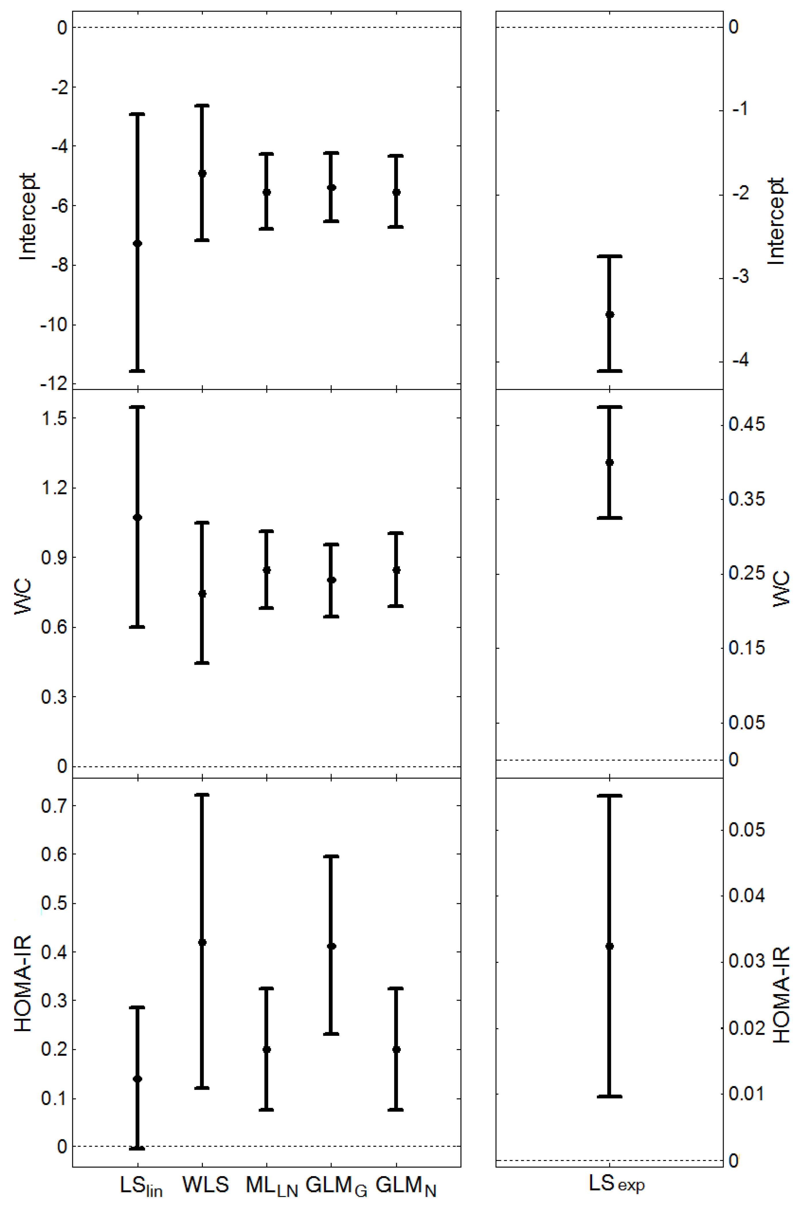
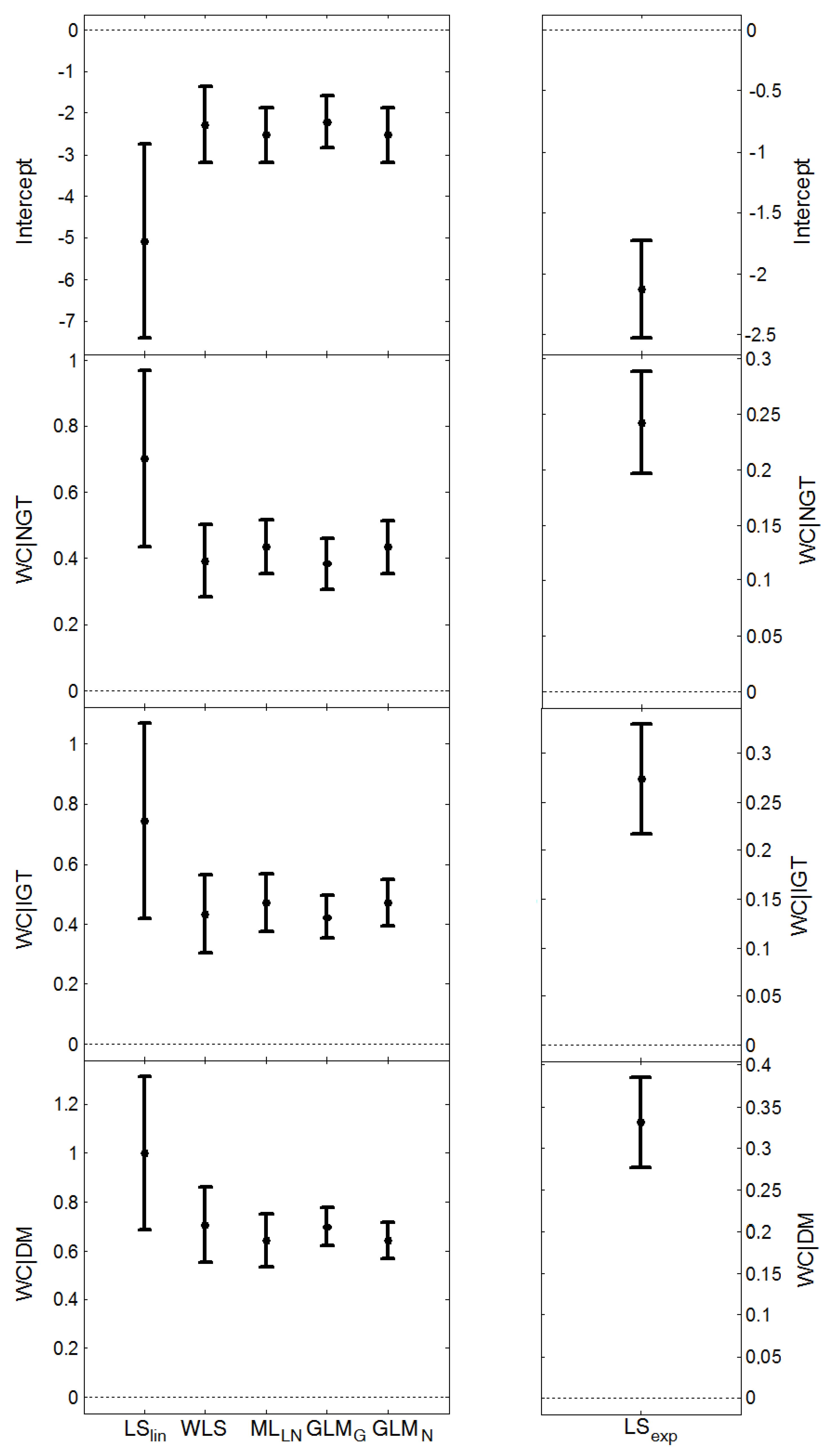
 , and the average length of the confidence intervals for μY, (estimated from the models presented in Figure 1 and Figure 2), are given in Table 6. MLLN, GLMN and LSexp gave similar estimates of σZ (this parameter cannot be estimated by LSlin). WLS provided the largest estimate whereas GLMG gave the smallest. MLLN and GLMG had similar confidence intervals for the expected value, μY, GLMN had the shortest intervals, whereas LSlin had the longest intervals.
| Method | CRP | HOMA-IR | |||
| | Length CI (mean, SD) | | Length CI (mean, SD) | ||
| LSlin | - | 1.61 (0.89) | - | 1.10 (0.19) | |
| WLS | 1.22 | 1.51 (2.07) | 0.73 | 0.64 (0.35) | |
| MLLN | 1.04 | 0.82 (0.86) | 0.61 | 0.43 (0.19) | |
| GLMG | 0.71 (0.974 1) | 0.85 (1.26) | 0.33 (2.52 1) | 0.47 (0.26) | |
| GLMN | 1.04 | 0.43 (0.23) | 0.61 | 0.23 (0.06) | |
| LSexp | 1.04 | 1.19 (5.40) | 0.60 | 0.50 (0.45) | |
3.2.2. Quantification of Factors Associated with CRP and HOMA-OR (Method Comparison)
4. Discussion
 and finally the common method based on log-transformation was included for comparison, μZǀX = δ0 + δ1X1 + … + δpXp. Evaluation was made both using simulations and by applying the methods to a large data set to estimate well-known associations of abdominal adiposity (waist circumference, WC) on inflammation (measured using C-reactive protein, CRP) and insulin resistance (measured using HOMA-IR), respectively.
4.1. Method Comparison
 , tended to be too small, thus overestimating the power. For LSlin, the assumption of a constant variance for Y resulted in confidence intervals for μY with unnecessary high coverage for small μY-values and too low coverage at large μY-values. LSexp does estimate the relative effect rather than the absolute and as a result the estimated expected values were biased and the coverage of the confidence intervals was erroneous. The confidence intervals from the GLMG method had too low coverage, as a result of the underestimation of the variance
  . This is contrary to the situation with a multiplicative model, where the gamma distribution often provide reasonable estimates when applied to a log-normal variable [41,42]. MLLN, WLS and GLMN provided approximately correct coverage, although GLMN had a tendency to underestimate, as a result of using the estimate , thus not including the stochastic variation of in the interval estimation. An approximate confidence interval taking into account its stochastic variation could be derived using Taylor expansion, see e.g. [43]., GLMG had narrower intervals than MLLN and GLMN for μY, but from the simulation we know that the coverage will be too low. Thus MLLN will have a higher power and for lognormal data the probability of detecting a true explanatory variable is higher. The smaller interval lengths of MLLN corroborate the results of a previous simulation study [11].
 4.2. Factors Associated with CRP and HOMA-IR, Respectively
4.3. Model Choice
4.4. Strengths and Weaknesses
5. Conclusions
Acknowledgments
Author Contributions
Conflicts of Interest
References
- Rappaport, S. Selection of the measures of exposure for epidemiology studies. Appl. Occup. Environ. Hyg. 1991, 6, 448–457. [Google Scholar] [CrossRef]
- Crump, K. On summarizing group exposures in risk assessment: Is an arithmetic mean or a geometric mean more appropriate? Risk Anal. 1998, 18, 293–297. [Google Scholar] [CrossRef]
- Rappaport, S. Assessment of long-term exposures to toxic substances in air. Ann. Occup. Hyg. 1991, 35, 61–121. [Google Scholar] [CrossRef]
- Koch, A. The logarithm in biology 1. Mechanisms generating the log-normal distribution exactly. J. Theor. Biol. 1966, 12, 276–290. [Google Scholar] [CrossRef]
- Osvoll, P.; Woldbæk, T. Distribution and skewness of occupational exposure sets of measurements in the Norwegian industry. Ann. Occup. Hyg. 1999, 43, 421–428. [Google Scholar]
- Limpert, E.; Stahel, W.; Abbt, M. Log-normal distributions across the sciences: Keys and clues. BioScience 2001, 51, 341–352. [Google Scholar] [CrossRef]
- Zhou, X.-H.; Stroupe, K.; Tierney, W. Regression analysis of health care charges with heteroscedasticity. J. R. Stat. Soc. Ser. C 2001, 50, 303–312. [Google Scholar]
- Rothman, K.J. Epidemiology. An Introduction; Oxford University Press Inc: New York, NY, USA, 2002. [Google Scholar]
- Rothman, K.J.; Greenland, S. Concepts of Interaction. In Modern Epidemiology, 2nd ed.; Rothman, K.J., Greenland, S., Eds.; Lippincott Williams and Wilkins: Philadelphia, PA, USA, 1998. [Google Scholar]
- McCullagh, P.; Nelder, J. Generalized Linear Models, 2nd ed.; CRC Press: Boca Raton, FL, USA, 1989. [Google Scholar]
- Gustavsson, S.; Johannesson, S.; Sallsten, G.; Andersson, E.M. Linear maximum likelihood regression analysis for untransformed log-normally distributed data. Open J. Stat. 2012, 2, 389–400. [Google Scholar] [CrossRef]
- Yurgens, Y. Quantifying Environmental Impact by Log-Normal Regression Modelling of Accumulated Exposure; Chalmers University of technology and Goteborg University: Goteborg, Sweden, 2004. [Google Scholar]
- Jensen, S.; Johansen, S.; Lauritzen, S. Globally convergent algorithms for maximizing likelihood function. Biometrika 1991, 78, 867–877. [Google Scholar]
- Niwitpong, S. Confidence intervals for the mean of a lognormal distribution. Appl. Math. Sci. 2013, 7, 161–166. [Google Scholar]
- Johannesson, S.; Gustafson, P.; Molnar, P.; Barregard, L.; Sallsten, G. Exposure to fine particles (PM2.5 and PM1) and black smoke in the general population: Personal, indoor, and outdoor levels. J. Expos. Sci. Environ. Epidemiol. 2007, 17, 613–624. [Google Scholar] [CrossRef]
- Englert, N. Fine particles and human health—A review of epidemiological studies. Toxicol. Letters 2004, 149, 235–242. [Google Scholar] [CrossRef]
- Dominici, F.; Peng, R.D.; Bell, M.L.; Pham, L.; McDermott, A.; Zeger, S.L.; Samet, J.M. Fine particulate air pollution and hospital admission for cardiovascular and respiratory diseases. J. Am. Med. Assoc. 2006, 295, 1127–1134. [Google Scholar] [CrossRef]
- Koistinen, K.J.; Hänninen, O.; Rotko, T.; Edwards, R.D.; Moschandreas, D.; Jantunen, M.J. Behavioral and environmental determinants of personal exposures to PM2.5 in EXPOLIS—Helsinki, Finland. Atmos. Environ. 2001, 35, 2473–2481. [Google Scholar] [CrossRef]
- Brohall, G.; Behre, C.-J.; Hulthe, J.; Wikstrand, J.; Fagerberg, B. Prevalence of diabetes and impaired glucose tolerance in 64-year-old swedish women. Diabetes Care 2006, 29, 363–367. [Google Scholar] [CrossRef]
- Fagerberg, B.; Kellis, D.; Bergström, G.; Behre, C.J. Adiponectin in relation to insulin sensitivity and insulin secretion in the development of type 2 diabetes: A prospective study in 64-year-old women. J. Int. Med. 2011, 269, 636–643. [Google Scholar] [CrossRef]
- Alberti, K.; Zimmet, P. Definition, diagnosis and classification of diabetes mellitus and its complications. Part 1: Diagnosis and classification of diabetes mellitus. Provisional report of a WHO consultation. Diabetic Med. 1998, 15, 539–553. [Google Scholar] [CrossRef]
- Ford, E.S. Body mass index, diabetes, and C-reactive protein among U.S. adults. Diabetes Care 1999, 22, 1971–1977. [Google Scholar] [CrossRef]
- Fröhlich, M.; Sund, M.; Löwel, H.; Imhof, A.; Hoffmeister, A.; Koenig, W. Independent association of various smoking characteristics with markers of systemic inflammation in men. Eur. Heart J. 2003, 24, 1365–1372. [Google Scholar] [CrossRef]
- Leinonen, E.; Hurt-Camejo, E.; Wiklund, O.; Hulten, L.M.; Hiukka, A.; Taskinen, M.R. Insulin resistance and adiposity correlate with acute-phase reaction and soluble cell adhesion molecules in type 2 diabetes. Atherosclerosis 2003, 166, 387–394. [Google Scholar] [CrossRef]
- O’Loughlin, J.; Lambert, M.; Karp, I.; McGrath, J.; Gray-Donald, K.; Barnett, T.A.; Delvin, E.E.; Levy, E.; Paradis, G. Association between cigarette smoking and C-reactive protein in a representative, population-based sample of adolescents. Nicot. Tob. Res. 2008, 10, 525–532. [Google Scholar]
- Reaven, G. Banting lecture 1988. Role of insulin resistance in human disease. Diabetes 1988, 37, 1595–1607. [Google Scholar] [CrossRef]
- Sites, C.K.; Calles-Escandón, J.; Brochu, M.; Butterfield, M.; Ashikaga, T.; Poehlman, E.T. Relation of regional fat distribution to insulin sensitivity in postmenopausal women. Fertil. Steril. 2000, 73, 61–65. [Google Scholar] [CrossRef]
- Wagenknecht, L.E.; Langefeld, C.D.; Scherzinger, A.L.; Norris, J.M.; Haffner, S.M.; Saad, M.F.; Bergman, R.N. Insulin sensitivity, insulin secretion, and abdominal fat. The insulin resistance atherosclerosis study (IRAS) family study. Diabetes 2003, 52, 2490–2496. [Google Scholar] [CrossRef]
- Facchini, F.S.; Hollenbeck, C.B.; Jeppesen, J.; Chen, Y.D.; Reaven, G.M. Insulin resistance and cigarette smoking. Lancet 1992, 339, 1128–1130. [Google Scholar] [CrossRef]
- Mayer-Davis, E.J.; D’Agostino, R., Jr.; Karter, A.J.; Haffner, S.M.; Rewers, M.J.; Mohammed, S.; Bergman, R.N.; for the IRAS Investigators. Intensity and amount of physical activity in relation to insulin sensitivity. J. Am. Med. Assoc. 1998, 279, 669–674. [Google Scholar] [CrossRef]
- Matthews, D.R.; Hosker, J.P.; Rudenski, A.S.; Naylor, B.A.; Treacher, D.F.; Turner, R.C. Homeostasis model assessment: Insulin resistance and β-cell function from fasting plasma glucose and insulin concentrations in man. Diabetologia 1985, 28, 412–419. [Google Scholar] [CrossRef]
- Taniguchi, A.; Fukushima, M.; Sakai, M.; Kataoka, K.; Nagata, I.; Doi, K.; Arakawa, H.; Nagasaka, S.; Toshikatsu, K.; Nakai, Y. The role of the body mass index and triglyceride levels in identifying insulin-sensitive and insulin-resistant variants in Japanese non-insulin-dependent diabetic patients. Metabolism 2000, 49, 1001–1005. [Google Scholar] [CrossRef]
- Radikova, Z.; Koska, J.; Huckova, M.; Ksinantova, L.; Imrich, R.; Trnovec, T.; Langer, P.; Sebokova, E.; Klimes, I. Insulin sensitivity indices: A proposal of cut-off points for simple identification of insulin-resistant subjects. Exp. Clin. Endocrinol. Diabetes 2006, 114, 249–256. [Google Scholar] [CrossRef]
- Geloneze, B.; Vasques, A.C.J.; Stabe, C.F.C.; Pareja, J.C.; de Lima Rosado, L.E.F.P.; de Queiroz, E.C.; Tambascia, M.A.; BRAMS Investigators. HOMA1-IR and HOMA2-IR indexes in identifying insulin resistance and metabolic syndrome: Brazilian metabolic syndrome study (BRAMS). Arq. Bra. Endocrinol. Metab. 2009, 53, 281–287. [Google Scholar] [CrossRef]
- Dickerson, E.H.; Cho, L.W.; Maguiness, S.D.; Killick, S.L.; Atkin, S.L. Insulin resistance and free androgen index correlate with the outcome of controlled ovarian hyperstimulation in non-PCOS women undergoing IVF. Hum. Reprod. 2010, 25, 504–509. [Google Scholar] [CrossRef]
- Land, C.E. An evaluation of approximate confidence interval estimation methods for lognormal means. Technometrics 1972, 14, 145–158. [Google Scholar] [CrossRef]
- Zhou, X.-H.; Gao, S.; Hui, S. Methods for comparing the means of two independent log-normal samples. Biometrics 1997, 53, 1129–1135. [Google Scholar] [CrossRef]
- Zou, G.Y.; Huo, C.Y.; Taleban, J. Simple confidence intervals for lognormal means and their differences with environmental applications. Environmetrics 2009, 20, 172–180. [Google Scholar] [CrossRef]
- Taylor, D.J.; Kupper, L.L.; Muller, K.E. Improved approximate confidence intervals for the mean of a log-normal random variable. Stat. Med. 2002, 21, 1443–1459. [Google Scholar] [CrossRef]
- Wu, J.; Wong, A.C.M.; Jiang, G. Likelihood-based confidence intervals for a log-normal mean. Stat. Med. 2003, 22, 1849–1860. [Google Scholar] [CrossRef]
- Firth, D. Multiplicative errors: Log-normal or gamma? J. R. Stat. Soc. Ser. B 1998, 50, 266–268. [Google Scholar]
- Das, R.N.; Park, J.-S. Discrepancy in regression estimates between log-normal and gamma: Some case studies. J. Appl. Stat. 2012, 39, 97–111. [Google Scholar] [CrossRef]
- Rade, L.; Westergran, B. Mathematics Handbook for Science and Engineering (BETA); Studentlitteratur: Lund, Sweden, 1998. [Google Scholar]
- Visser, M.; Bouter, L.M.; McQuillan, G.M.; Wener, M.H.; Harris, T.B. Elevated C-reactive protein levels in overweight and obese adults. J. Am. Med. Assoc. 1999, 282, 2131–2135. [Google Scholar] [CrossRef]
- Yudkin, J.S.; Stehouwer, C.D.A.; Emeis, J.J.; Coppack, S.W. C-Reactive protein in healthy subjects: Associations with obesity, insulin resistance, and endothelial dysfunction. A potential role for cytokines originating from adipose tissue? Arterioscler. Thromb. Vasc. Biol. 1999, 19, 972–978. [Google Scholar] [CrossRef]
- Pannacciulli, N.; Cantatore, F.P.; Minenna, A.; Bellacicco, M.; Giorgino, R.; de Pergola, G. C-reactive protein is independently associated with total body fat, central fat, and insulin resistance in adult women. Int. J. Obes. Relat. Metab. Disord. 2001, 25, 1416–1420. [Google Scholar] [CrossRef]
- McLaughlin, T.; Abbasi, F.; Lamendola, C.; Liang, L.; Reaven, G.; Schaaf, P.; Reaven, P. Differentiation between obesity and insulin resistance in the association with C-reactive protein. Circulation 2002, 106, 2908–2912. [Google Scholar] [CrossRef]
- Lapice, E.; Maione, S.; Patti, L.; Cipriano, P.; Rivellese, A.A.; Riccardi, G.; Vaccaro, O. Abdominal adiposity is associated with elevated C-reactive protein independent of bmi in healthy nonobese people. Diabetes Care 2009, 32, 1734–1736. [Google Scholar] [CrossRef]
- Brooks, G.; Blaha, M.; Blumenthal, R. Relation of C-reactive protein to abdominal adiposity. Am. J. Cardiol. 2010, 106, 56–61. [Google Scholar] [CrossRef]
- Hermsdorff, H.H.M.; Zulet, M.A.; Puchau, B.; Martinez, J.A. Central adiposity rather than total adiposity measurements are specifically involved in the inflammatory status from healthy young adults. Inflammation 2011, 34, 161–170. [Google Scholar] [CrossRef]
- Hak, A.E.; Stehouwer, C.D.A.; Bots, M.L.; Polderman, K.H.; Schalkwijk, C.G.; Westendorp, I.C.D.; Hofman, A.; Witteman, J.C.M. Associations of C-reactive protein with measures of obesity, insulin resistance, and subclinical atherosclerosis in healthy, middle-aged women. Arterioscler. Thromb. Vasc. Biol. 1999, 19, 1986–1991. [Google Scholar] [CrossRef]
- Festa, A.; D’Agostino, R., Jr.; Howard, G.; Mykkanen, L.; Tracy, R.P.; Haffner, S.M. Chronic subclinical inflammation as part of the insulin resistance syndrome: The insulin resistance atherosclerosis study (IRAS). Circulation 2000, 102, 42–47. [Google Scholar] [CrossRef]
- Lemieux, I.; Pascot, A.; Prud’homme, D.; Almeras, N.; Bogaty, P.; Nadeau, A.; Bergeron, J.; Despres, J.-P. Elevated C-reactive protein : Another component of the atherothrombotic profile of abdominal obesity. Arterioscler. Thromb. Vasc. Biol. 2001, 21, 961–967. [Google Scholar] [CrossRef]
- Wallace, T.M.; Levy, J.; Matthews, D. Use and abuse of HOMA modeling. Diabetes Care 2004, 27, 1487–1495. [Google Scholar] [CrossRef]
- Huang, L.-H.; Liao, Y.-L.; Hsu, C.-H. Waist circumference is a better predictor than body mass index of insulin resistance in type 2 diabetes. Obes. Res. Clin. Pract. 2011, 6, e314–e320. [Google Scholar] [CrossRef]
- Lee, K. Usefulness of the metabolic syndrome criteria as predictors of insulin resistance among obese Korean women. Public Health Nutr. 2010, 13, 181–186. [Google Scholar] [CrossRef]
- Thomas, D.C. General relative-risk models for survival time and matched case-control analysis. Biometrics 1981, 37, 673–686. [Google Scholar] [CrossRef]
- Richardson, D.B.; Langholz, B. Background stratified poisson regression analysis of cohort data. Radiat. Environ. Biophys. 2012, 51, 15–22. [Google Scholar] [CrossRef]
- Rothman, K.J. Causes. Am. J. Epidemiol. 1976, 104, 587–592. [Google Scholar]
- VanderWeele, T.J. On the distinction between interaction and effect modification. Epidemiology 2009, 20, 863–871. [Google Scholar] [CrossRef]
- Nurminen, M. To use or not to use the odds ratio in epidemiologic analyses? Eur. J. Epidemiol. 1995, 11, 365–371. [Google Scholar] [CrossRef]
- Andersson, T.; Alfredsson, L.; Kallberg, H.; Zdravkovic, S.; Ahlbom, A. Calculating measures of biological interaction. Eur. J. Epidemiol. 2005, 20, 575–579. [Google Scholar] [CrossRef]
© 2014 by the authors; licensee MDPI, Basel, Switzerland. This article is an open access article distributed under the terms and conditions of the Creative Commons Attribution license (http://creativecommons.org/licenses/by/3.0/).
Share and Cite
Gustavsson, S.; Fagerberg, B.; Sallsten, G.; Andersson, E.M. Regression Models for Log-Normal Data: Comparing Different Methods for Quantifying the Association between Abdominal Adiposity and Biomarkers of Inflammation and Insulin Resistance. Int. J. Environ. Res. Public Health 2014, 11, 3521-3539. https://doi.org/10.3390/ijerph110403521
Gustavsson S, Fagerberg B, Sallsten G, Andersson EM. Regression Models for Log-Normal Data: Comparing Different Methods for Quantifying the Association between Abdominal Adiposity and Biomarkers of Inflammation and Insulin Resistance. International Journal of Environmental Research and Public Health. 2014; 11(4):3521-3539. https://doi.org/10.3390/ijerph110403521
Chicago/Turabian StyleGustavsson, Sara, Björn Fagerberg, Gerd Sallsten, and Eva M. Andersson. 2014. "Regression Models for Log-Normal Data: Comparing Different Methods for Quantifying the Association between Abdominal Adiposity and Biomarkers of Inflammation and Insulin Resistance" International Journal of Environmental Research and Public Health 11, no. 4: 3521-3539. https://doi.org/10.3390/ijerph110403521
APA StyleGustavsson, S., Fagerberg, B., Sallsten, G., & Andersson, E. M. (2014). Regression Models for Log-Normal Data: Comparing Different Methods for Quantifying the Association between Abdominal Adiposity and Biomarkers of Inflammation and Insulin Resistance. International Journal of Environmental Research and Public Health, 11(4), 3521-3539. https://doi.org/10.3390/ijerph110403521