Scalable Combinatorial Tools for Health Disparities Research


 ,
,
Abstract
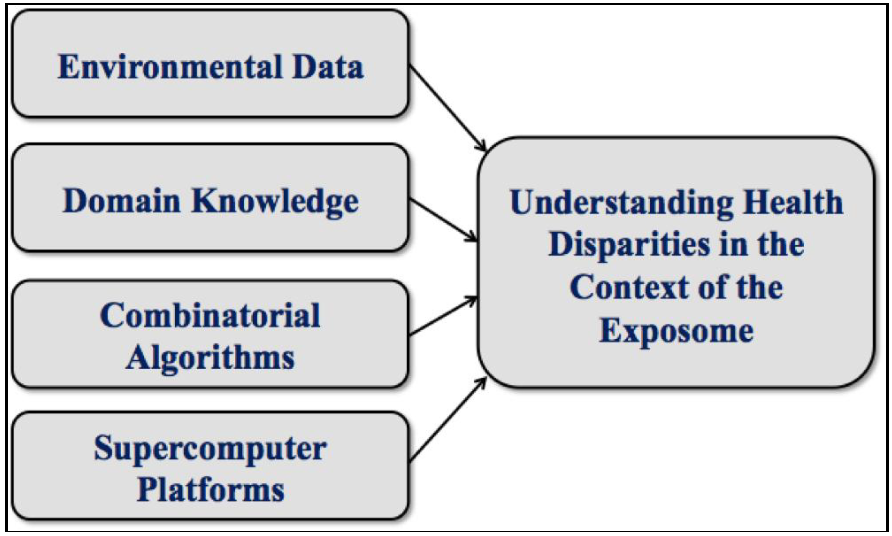
:1. Background
2. Introduction

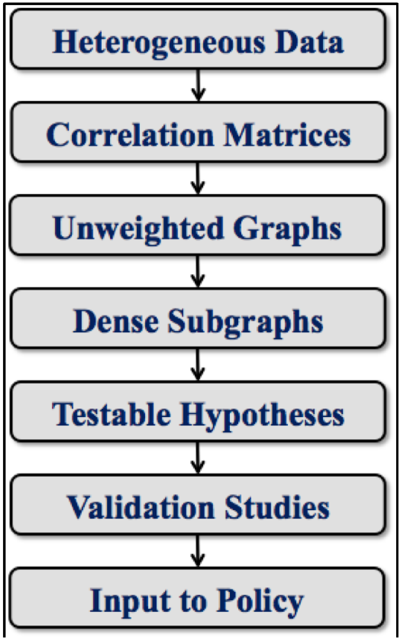
3. Graph Theoretical Utility
4. Graph Algorithmic Methods

5. Supporting Technologies
6. Analytical Toolchain

7. Refinements and Variations
- Feature Selection can aid in early dimension reduction by eliminating irrelevant variables and bringing focus to the most important regions of the input space [21]. In the extreme case, one might even eliminate all variables or readings not associated with a single outcome.
- Fuzzy Computations are often preferred, in an effort to counteract or at least ameliorate the effects of noise. Examples include soft thresholding and near-clique extractions [25].
- Subgraph Overlap may increase fidelity. By tuning our codes to provide this feature, a vertex may reside in more than one subgraph, just as a variable may be involved in more than one relationship [26].
- Domain Knowledge, usually invoked only at toolchain extremes, can sometimes be applied midstream. Subgraphs can be anchored at variables of established significance. Thresholds can be set using specific knowledge of variable-variable interaction strengths.
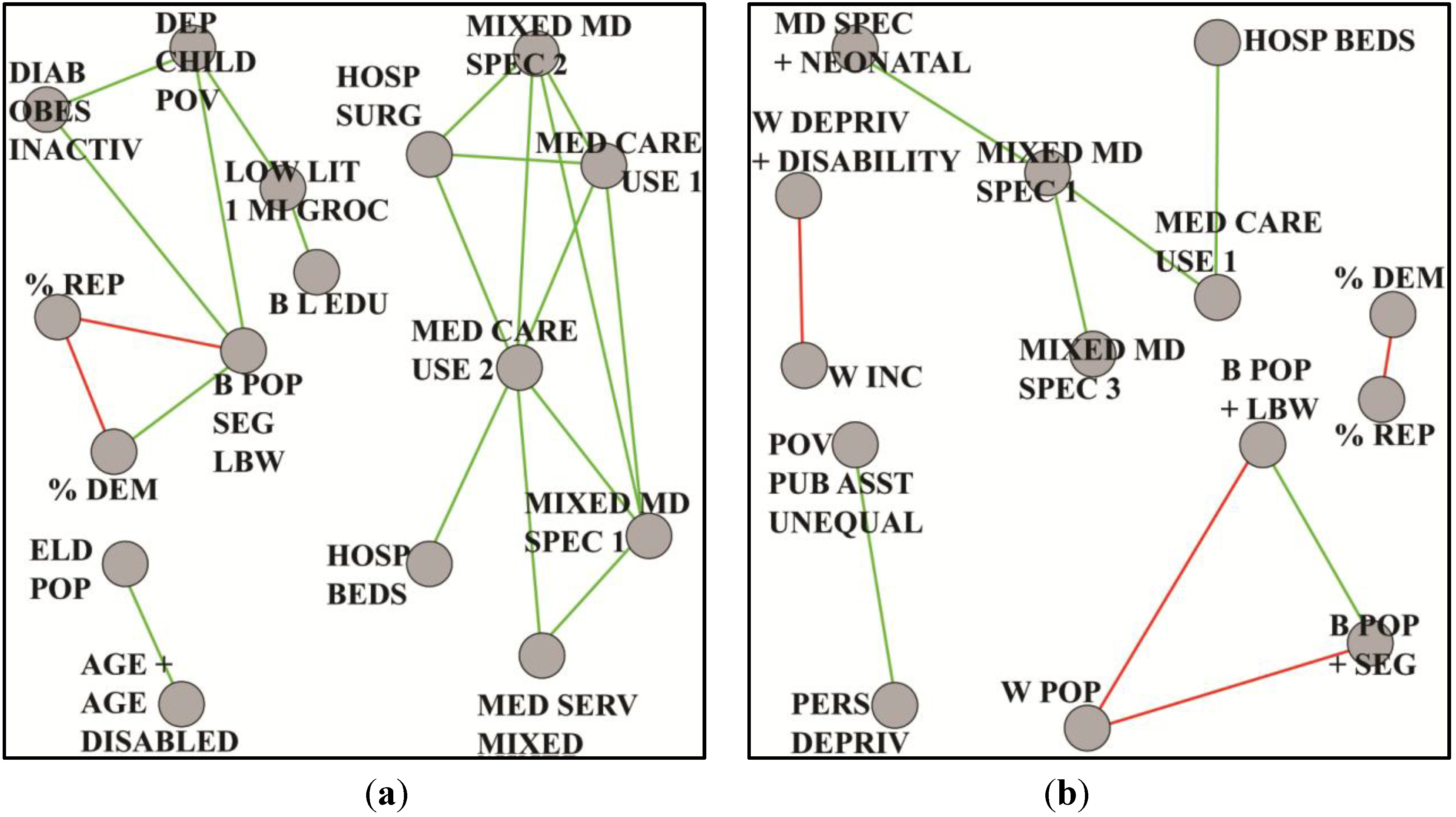
8. Exemplars

| Exemplar | Prematurity | Longevity | Lung Cancer |
|---|---|---|---|
| Study Design | One Case | Two Case | Eight Case |
| Selection Basis | Population | Mortality | Race, Sex, Mortality |
| Refinement | ------ | ------ | ANOVA |
| Hypothesis Generation | Stand-Alone | Differential | Differential |
| Traditional Verification | Bayesian Analysis | ------ | ------ |
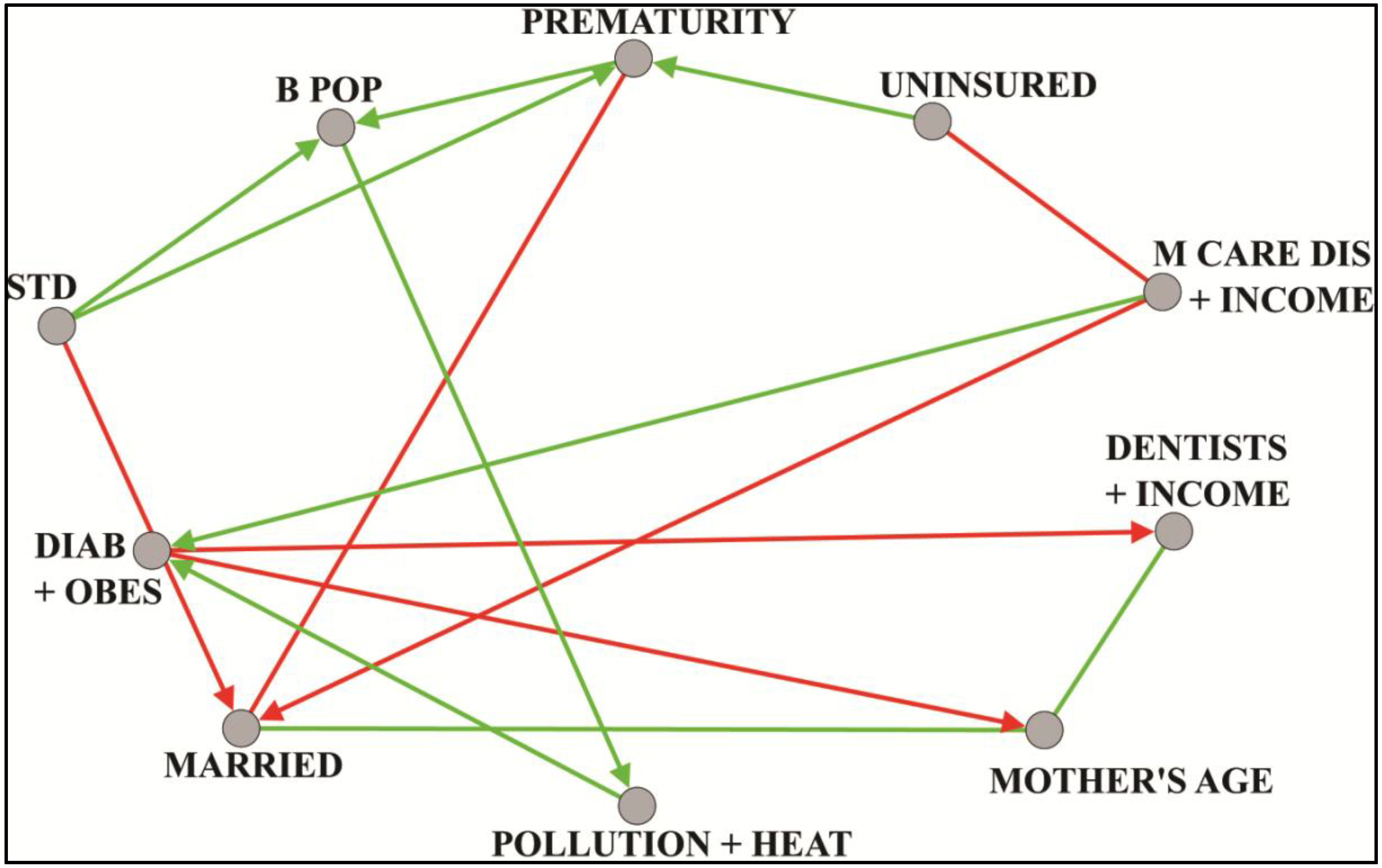
8.1. Prematurity
8.2. Longevity
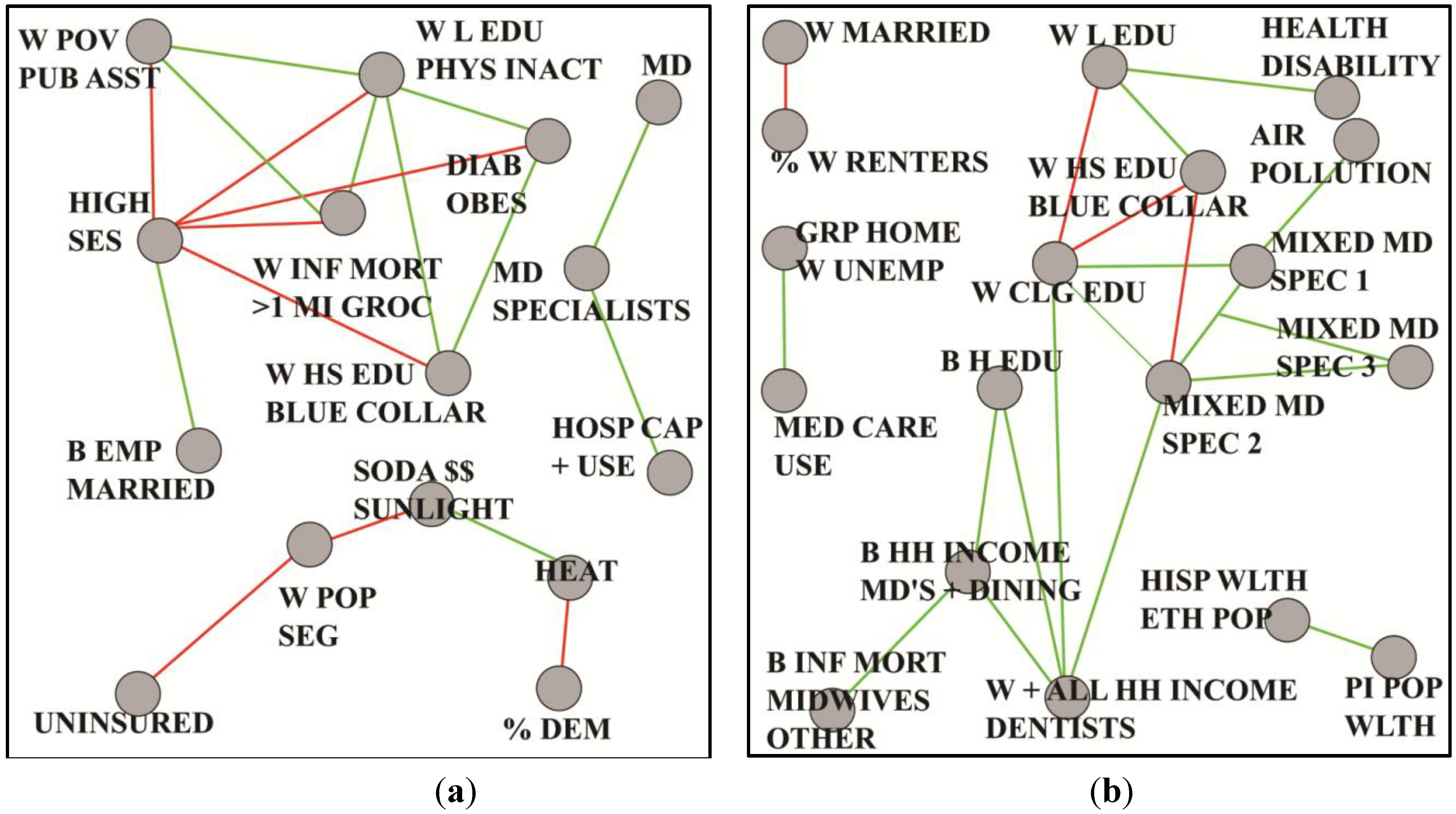
8.3. Lung Cancer

9. Limitations
10. Conclusions
11. Directions for Future Research
Acknowledgments
Author Contributions
Conflicts of Interest
References
- Juarez, P.D. Sequencing the public health genome. J. Health Care Poor Underserved. 2013, 24, 114–120. [Google Scholar] [CrossRef] [PubMed]
- Wild, C.P. Complementing the genome with an “Exposome”: The outstanding challenge of environmental exposure measurement in molecular epidemiology. Cancer Epidem. Biomarker Prev. 2005, 14, 1847–1850. [Google Scholar] [CrossRef]
- Matthews-Juarez, P. Developing a cadre of transdisciplinary health disparities researchers for the 21st century. J. Health Care Poor Underserved. 2013, 24, 121–128. [Google Scholar] [CrossRef] [PubMed]
- Kuhn, T. The Structure of Scientific Revolutions; University of Chicago Press: Chicago, IL, USA, 1962; pp. 1–199. [Google Scholar]
- Khoury, M.J.; Lam, T.K.; Ioannidis, J.P.; Hartge, P.; Spitz, M.R.; Buring, J.E.; Chanock, S.J.; Croyle, R.T.; Goddard, K.A.; Ginsburg, G.S.; et al. Transforming epidemiology for 21st century medicine and public health. Cancer Epidem. Biomarker Prev. 2013, 22, 508–516. [Google Scholar] [CrossRef]
- Juarez, P.D.; Hood, D.B.; Im, W.; Levine, R.S.; Matthews-Juarez, P.; Kilbourne, B.J.; Langston, M.A.; Alhamdan, M.Z.; Agboto, V.; Crosson, W.L.; et al. The public health exposome: A population-based, health disparities, exposure science approach to appear. Int. J. Environ. Res. Public Health 2014. under review. [Google Scholar]
- Adler, N.; Bush, N.R.; Pantell, M.S. Rigor, vigor, and the study of health disparities. Proc. Natl. Acad. Sci. USA 2012, 109, 17154–17159. [Google Scholar] [CrossRef] [PubMed]
- Butte, A.J.; Tamayo, P.; Slonim, D.; Golub, T.R.; Kohane, I.S. Discovering functional relationships between rna expression and chemotherapeutic susceptibility using relevance networks. Proc. Natl. Acad. Sci. USA 2000, 97, 12182–12186. [Google Scholar] [CrossRef] [PubMed]
- Wolfe, C.J.; Kohane, I.S.; Butte, A.J. Systematic survey reveals general applicability of “Guilt-by-Association” within gene coexpression networks. BMC Bioinformatics 2005, 6. [Google Scholar] [CrossRef] [PubMed]
- Euler, L. Solutio problematis ad geometriam situs pertinentis. Comment. Academ. Sci. Petropolit. 1741, 8, 128–140. [Google Scholar]
- West, D.B. Introduction to Graph Theory; Pearson: Upper Saddle River, NJ, USA, 2000; pp. 1–470. [Google Scholar]
- Block, R. Community, environment and violent crime. Criminology 1979, 17, 46–57. [Google Scholar] [CrossRef]
- Bomze, I.; Budinich, M.; Pardalos, P.; Pelillo, M. The maximum clique problem. In Handbook of Combinatorial Optimization; Du, D.-Z., Pardalos, P.M., Eds.; Kluwer Academic Publishers: New York, NY, USA, 1999; Vol. 4. [Google Scholar]
- Garey, M.R.; Johnson, D.S. Computers and Intractability. A Guide to the Theory of NP-Completeness; W.H. Freeman and Company: San Francisco, CA, USA, 1979. [Google Scholar]
- Abu-Khzam, F.N.; Langston, M.A.; Shanbhag, P.; Symons, C.T. Scalable parallel algorithms for FPT problems. Algorithmica 2006, 45, 269–284. [Google Scholar] [CrossRef]
- Borate, B.R.; Chesler, E.J.; Langston, M.A.; Saxton, A.M.; Voy, B.H. Comparative analysis of thresholding approaches for microarray-derived gene co-expression matrices. BMC Res. Note. 2009, 2. [Google Scholar] [CrossRef]
- Perkins, A.D.; Langston, M.A. Threshold selection in gene co-expression networks using spectral graph theory techniques. BMC Bioinformatics 2009, 10. [Google Scholar] [CrossRef] [PubMed]
- Faisandier, L.; Bonneterre, V.; de Gaudemaris, R.; Bicout, D.J. A Network-Based Approach for Surveillance of Occupational Health Exposures. Available online: http://arxiv.org/abs/arxiv:0907.3355 (accessed on 8 October 2014).
- Langston, M.A.; Perkins, A.D.; Saxton, A.M.; Scharff, J.A.; Voy, B.H. Innovative computational methods for transcriptomic data analysis: A case study in the use of FPT for practical algorithm design and implementation. Comput. J. 2008, 51, 26–38. [Google Scholar] [CrossRef]
- Voy, B.H.; Scharff, J.A.; Perkins, A.D.; Saxton, A.M.; Borate, B.; Chesler, E.J.; Branstetter, L.K.; Langston, M.A. Extracting gene networks for low dose radiation using graph theoretical algorithms. PLoS Comput. Biol. 2006, 2. [Google Scholar] [CrossRef]
- Guyon, I.; Elisseeff, A. An introduction to variable and feature selection. J. Mach. Learn. Res. 2003, 3, 1157–1182. [Google Scholar]
- Fisher, R.A. The distribution of the partial correlation coefficient. Metron 1924, 3, 329–332. [Google Scholar]
- Everitt, B.S.; Skrondal, A. The Cambridge Dictionary of Statistics; Cambridge University Press: Cambridge, UK, 2010; pp. 1–478. [Google Scholar]
- Wong, F.; Carter, C.K.; Kohn, R. Efficient estimation of covariance selection models. Biometrika 2003, 90, 809–830. [Google Scholar] [CrossRef]
- Chesler, E.J.; Langston, M.A. Combinatorial genetic regulatory network analysis tools for high throughput transcriptomic data. In Systems Biology and Regulatory Genomics; Eskin, E., Ed.; Springer: Berlin, Germany, 2006; Vol. 4023, pp. 150–165. [Google Scholar]
- Eblen, J.D.; Gerling, I.C.; Saxton, A.M.; Wu, J.; Snoddy, J.R.; Langston, M.A. Graph algorithms for integrated biological analysis, with applications to type 1 diabetes data. In Clustering Challenges in Biological Networks; Chaovalitwongse, W.A., Ed.; World Scientific: Singapore, 2009; pp. 207–222. [Google Scholar]
- Chen, C.K.; Matthews-Juarez, P.; Yang, A. Effect of hurricane Katrina on low birth weight and preterm deliveries in African American women in Louisiana, Mississippi, and Alabama. J. Syst. Cybnernet. Inform. 2012, 10, 102–107. [Google Scholar]
- Lu, M.; Kotelchuck, M.; Hogan, V.; Jones, L.; Wright, K.; Halfon, N. Closing the Black-White gap in birth outcomes: A life-course approach. Ethn. Dis. 2010, 20, S2-62–S2-76. [Google Scholar] [PubMed]
- Bryant, A.S.; Worjoloh, A.; Caughey, A.B.; Washington, A.E. Racial/ethnic disparities in obstetric outcomes and care: Prevalence and determinants. Amer. J. Obstet. Gynecol. 2010, 202, 335–343. [Google Scholar] [CrossRef]
- MacDorman, M.F.; Mathews, T. Understanding Racial and Ethnic Disparities in U.S Infant Mortality Rates; National Center for Health Statistics: Hyattsville, MD, USA, 2011. [Google Scholar]
- Payne-Sturges, D.; Gee, C. National environmental health measures for minority and low-income populations: Tracking social disparities in environmental health. Environ. Res. 2006, 102, 154–171. [Google Scholar] [CrossRef] [PubMed]
- Kershenbaum, A.D.; Langston, M.A.; Levine, R.S.; Saxton, A.M.; Oyana, T.J.; Kilbourne, B.J.; Rogers, G.L.; Gittner, L.; Backtash, S.H.; Matthews-Juarez, P.; Juarez, P.D. Exploration of premature birth rates using the public health exposome database and computational analysis methods. Int. J. Environ. Res. Public Health 2014. to be submitted. [Google Scholar]
- Levine, R.S.; Rust, G.; Aliyu, M.; Pisu, M.; Zoorob, R.; Goldzweig, I.; Juarez, P.; Husaini, B.; Hennekens, C.H. United States counties with low Black male mortality rates. Amer. J. Med. 2013, 126, 76–80. [Google Scholar] [CrossRef] [PubMed]
- Levine, R.S.; Kilbourne, B.J.; A, M.S.; Rogers, G.L.; Langston, M.A. Comparing social structures between communities with high and low Black male mortality. Int. J. Environ. Res. Public Health 2014. to be submitted. [Google Scholar]
- Aizer, A.A.; Wilhite, T.J.; Chen, M.H.; Graham, P.L.; Choueiri, T.K.; Hoffman, K.E.; Martin, N.E.; Trinh, Q.D.; Hu, J.C.; Nguyen, P.L. Lack of reduction in racial disparities in cancer-specific mortality over a 20-year period. Cancer 2014, 120, 1532–1539. [Google Scholar] [CrossRef] [PubMed]
- Howlader, N.; Noone, A.M.; Krapcho, M.; Garshell, J.; Miller, D.; Altekruse, S.F.; Kosary, C.L.; Yu, M.; Ruhl, J.; Tatalovich, Z.; et al. SEER Cancer Statistics Review, 1975–2011; National Cancer Institute: Bethesda, MD, USA, 2014. [Google Scholar]
- Pruitt, K. Too Many Cases, Too Many Deaths; American Lung Association: Washington, D.C., USA, 2010. [Google Scholar]
- Millsap, R.E. Confirmatory measurement model comparisons using latent means. Multivariate Behav. Res. 1991, 26. [Google Scholar] [CrossRef]
- Kilbourne, B.J.; Baktash, S.H.; Saxton, A.M.; G.L. Rogers, J.; Cao, G.; Langston, M.A.; Levine, R.S. Comparing the structure of health care and community SES to elucidate race and gender disparities in lung cancer mortality. Int. J. Environ. Res. Public Health 2014. to be submitted. [Google Scholar]
- Hennekens, C.H.; Buring, J.E. Epidemiology in Medicine; Little, Brown & Co.: Boston, MA, USA, 1987; pp. 1–383. [Google Scholar]
- Chan, K.S.; Fowles, J.B.; Weiner, J.P. Electronic health records and the reliability and validity of quality measures: A review of the literature. Med. Care Res. Rev. 2010, 67, 503–527. [Google Scholar] [CrossRef] [PubMed]
- Hoffman, S.; Podgurski, A. The use and misuse of big medical data: Is bigger really better? Amer. J. Law Med. 2013, 39, 497–538. [Google Scholar]
- Moscou, S.; Anderson, M.R.; Kaplan, J.B.; Valencia, L. Validity of racial/ethnic classifications in medical records data: An exploratory study. Amer. J. Public Health 2003, 93, 1084–1086. [Google Scholar] [CrossRef]
- Srebotnjak, T.; Mokdad, A.H.; Murray, J.J. A novel framework for validating and applying standardized small area measurement strategies. Popul. Health Metrics 2010, 8, 1–13. [Google Scholar] [CrossRef]
- Citro, C.; Kalton, G. Using the American Community Survey: Benefits and Challenges; The National Academies Press: Washington, DC, USA, 2007. [Google Scholar]
- Exposure Evaluation: Evaluating Environmental Contamination, Public Health Assessment Guidance Manual; Agency for Toxic Substances and Disease Registry: Atlanta, GA, USA, 2005; pp. 5-1–5-25.
- Arrandale, V.H.; Brauer, M.; Brook, J.R.; Brunekreef, B.; Gold, D.R.; London, S.J.; Miller, D.; Ozkaynak, H.; Ries, N.M.; Sears, M.R.; et al. Exposure assessment in cohort studies of childhood asthma. Environ. Health Perspect. 2011, 119, 591–597. [Google Scholar] [CrossRef] [PubMed]
- Geronimus, A.; Bound, J.; Neidert, J.A. On the Validity of Using Census Geocode Characteristics to Proxy Individual Socioeconomic Characteristics. J. Amer. Statist. Assn. 1996, 91, 529–537. [Google Scholar]
- Krieger, N.; Chen, J.T.; Waterman, P.D.; Mah-Jabeen, S.; Subramanian, S.V.; Carson, R. Geocoding and monitoring of U.S. socioeconomic inequalities in mortality and cancer incidence: Does the choice of area-based measure and geographic level matter? Amer. J. Epidemiol. 2002, 156, 471–482. [Google Scholar]
- Schwartz, S. The fallacy of the ecological fallacy: The potential misuse of a concept and the consequences. Amer. J. Public Health 1994, 84, 819–824. [Google Scholar] [CrossRef]
- Harrell, F.E., Jr; Lee, K.L.; Califf, R.M.; Pryor, D.B.; Rosati, R.A. Regression modelling strategies for improved prognostic prediction. Stat. Med. 1984, 3, 143–152. [Google Scholar] [CrossRef] [PubMed]
- Peduzzi, P.; Concato, J.; Kemper, E.; Holford, T.R.; Feinstein, A.R. A simulation study of the number of events per variable in logistic regression analysis. J. Clin. Epidemiol. 1996, 12, 1373–1379. [Google Scholar] [CrossRef]
- Gelman, A.; Hill, J.; Yajima, M. Why we (usually) don’t have to worry about multiple comparisons. J. Res. Educ. Effectiveness 2012, 5, 189–211. [Google Scholar] [CrossRef]
- Genovese, C.R.; Roeder, K.; Wasserman, L. False discovery control with p-value weighting. Biometrika 2006, 93, 509–524. [Google Scholar] [CrossRef]
- Rubin, D.; Dudoit, S.; van der Laan, M.J. A Method to increase the power of multiple testing procedures through sample splitting. Stat. Appl. Genet. Mol. Biol. 2006, 5. [Google Scholar] [CrossRef]
- Benjamini, Y.; Hochberg, Y. Controlling the false discovery rate: A practical and powerful approach to multiple testing. J. Roy. Statist. Soc. Ser. B 1995, 57, 289–300. [Google Scholar]
- Genovese, C.R.; Wasserman, L. Operating characteristics and extensions of the false discovery rate procedure. J. Roy. Statist. Soc. Ser. B 2002, 64, 499–517. [Google Scholar] [CrossRef]
- McClellan, J.; King, M.C. Genetic heterogeneity in human disease. Cell 2010, 141, 210–217. [Google Scholar] [CrossRef] [PubMed]
Appendix
| Label | Variables | Meaning |
|---|---|---|
| B POP | 3 | black proportion and black isolation index |
| DIAB + OBES | 4 | diabetes, obesity and inactivity rates |
| DENTISTS+ INCOME | 2 | per capita income and dentists private practice |
| MARRIED | 2 | percentage married mothers |
| MCARE DIS+ INCOME | 4 | medicare enrollment and disabled and white median household income |
| MOTHER‘S AGE | 2 | mother age and births to mothers over age 40 |
| POLLUTION+ HEAT | 2 | pollution heat index and normalized fine particulate matter |
| PREMATURITY | 1 | logit of premature singleton birth proportion |
| STD | 2 | diagnosed cases of sexually transmitted diseases per population size: chlamydia and gonorrhea |
| UNINSURED | 2 | percent less than age 65 without health insurance, females and population total |
| Label | Variables | Meaning |
|---|---|---|
| % DEM | 3 | percent voters registered as Democrats, voted Democrat in 2004 election and voted Democrat in 2008 election |
| B EMP + MARRIED | 3 | rate black males age 16–64 employed, percent blacks and black males married |
| DIAB + OBES | 3 | percent residents diabetic and obese |
| HEAT | 5 | number of days with temperatures at least 90 degrees, average maximum temperature, average minimum temperature and average land surface temperature |
| HIGH SES | 12 | percent black and white adults with at least a four year degree, percent workers employed white collar occupations, median household income and per capita income |
| HOSP CAP + USE | 13 | rates per 1000 residents: hospital admissions, inpatient and outpatient surgeries, operating room and hospital beds |
| MD | 8 | rates per 1000 residents: primary and specialty care MD’s involved in patient care |
| MD SPECIALISTS | 5 | rates per 1000 residents: MD’s including surgical specialists, thoracic surgeons and urologists |
| SODA$$ + SUNLIGHT | 3 | average price 12 oz soda and average direct solar radiation in kilojoules per square meter |
| UNINSURED | 3 | percent population less than age 65 without health insurance |
| W HS EDU + BLUE COLLAR | 3 | percent female adults with only HS education and percent whites and white males employed in blue collar occupations |
| W INF MORT >1 MILE GROC | 3 | white infant mortality rate, percent low income residents residing more than 1 mile from grocery and households with no vehicle more than 1 mile from grocery |
| W L EDU + PHYS INACT | 4 | percent whites adults with less than HS education and percent residents classified as physically inactive |
| W POP + SEG | 2 | percent population non-Hispanic and white isolation index |
| W POV + PUB ASST | 7 | percent total and males Medicaid eligible, households on foodstamps and individuals less than age 18 in poverty |
| Label | Variables | Meaning |
|---|---|---|
| %W RENTERS | 2 | percent white households renters |
| AIR POLLUTION | 4 | particulate matter pollution, nitrous and nitrogen oxides |
| B H EDU | 3 | percent black adults with at least a four year degree |
| B HH INCOME + MD'S + DINING | 5 | median black household income, rate per 1000 residents MD’s in private practice and MD’s in other specialties, and percent restaurants full service |
| B INF MORT + MIDWIVES + OTHER | 4 | rate per 1000 residents midwives and recreational facilities, black infant mortality rate and percent change in households on foodstamps |
| GRP HOME + W UNEMP | 3 | percent population in group homes, white unemployment rate and rate per 1000 residents long term care beds |
| HEALTH + DISABILITY | 4 | average subjective health for residents and percent population qualifying for social security disability |
| HISP WLTH + ETH POP | 4 | percent population non-Hispanic Asian, percent Hispanic households owning homes valued more than 400 percent median U.S. value, percent population older than age 18, non English speakers and percent population foreign born |
| MED CARE USE | 8 | rates per 1000 residents: hospital admissions, inpatient and outpatient surgeries, operating rooms and intensive care beds |
| MIXED MD SPEC1 | 13 | rates per 1000 residents: total active MD’s, specialists (e.g., neurology, cardiology , surgical specialists and pathologists) |
| MIXED MD SPEC2 | 7 | rates per 1000 residents: office based MD’s, pediatricians, internists, psychiatrists, child psychiatrists and white per capita income |
| MIXED MD SPEC3 | 4 | rates per 1000: MD diagnostic radiologists, orthopedic surgeons, gastroenterologists and anesthesiologists |
| PI POP WLTH | 3 | percent population non-Hispanic Pacific Islanders and percent black and white households owning homes valued more than 400 percent median U.S. value |
| W CLG EDU | 2 | percent white adults with at least a four year degree |
| W HS EDU + BLUE COLLAR | 3 | percent total white and white male workers employed in blue collar occupations and percent adult males with HS education only |
| W L EDU | 3 | percent white adults with less than HS education |
| W MARRIED | 2 | percent white and white females married |
| W + ALL HH INC + DENTISTS | 4 | white and total median household income and rate per 1000 residents active dentists |
| Label | Variables | Meaning |
|---|---|---|
| %DEM | 3 | percent voters registered or voted Democratic 2004–2008 |
| %REP | 3 | percent voters registered or voted Republican 2004–2008 |
| AGE + AGE DISABLED | 8 | median age female, white non-Hispanic, non-Hispanic male, percent medicare enrolled aged, disabled, percent white males age 65 plus |
| B L EDU | 4 | rate black low education, education less than HS in blacks, education low black female and male |
| B POP + SEG + LBW | 4 | black isolation index 2000, low birth weight, percent non-Hispanic blacks 2008, percent black/African-American population |
| DEP CHILD POV | 9 | rate unmarried, percent free lunch, poverty less than age 18, foodstamp recipients; medicaid eligible female/male/total, poverty rate under age 18 |
| DIAB + OBES + INACTIV | 4 | percent diabetes in adults, percent obese adults, adjusted percent inactive, age-adjusted obesity 2009 |
| ELD POP | 3 | percent residents over age 65, eligible for Medicare and Medicare disability |
| HOSP BEDS | 3 | rate hospital beds: licensed, community hospital, hospital, licensed short term, short term, total inpatient |
| HOSP SURG | 3 | rate operating rooms, intensive care beds, medical-surgical adult beds |
| LOW LIT MI GROC | 3 | percent low literacy, percent low income over 10 miles to store 2006, percent households no car over 1 mile to store 2006, percent low income more than 10 miles to store 2006 |
| MED CARE USE 1 | 5 | rates per 1000 residents: outpatient visits, outpatient and total surgeries, medical-surgical pediatric beds |
| MED CARE USE 2 | 3 | rates per 1000 residents: community hospital admission, hospital admission, short term hospital admission |
| MED SERV MIXED | 4 | rate total MD’s family medicine, cardiology intensive care beds, neonatal intensive beds, total thoracic surgery beds |
| MIXED MD SPEC1 | 27 | rate mixed medical specialties |
| MIXED MD SPEC2 | 6 | rate per 1000 residents: MDs, gastroenterologists, ob-gynecologists, opthomologists and otoloryngologists |
| Label | Variables | Meaning |
|---|---|---|
| %DEM | 3 | percent voters registered or voted Democratic 2004–2008 |
| %REP | 3 | percent voters registered or voted Republican 2004–2008 |
| B POP + LBW | 6 | black isolation index 2000, low birth weight, percent non-Hispanic blacks 2008, percent black/African-American population, unmarried and very low birth weight |
| B POP + SEG | 3 | black isolation index 2000, percent non-Hispanic blacks 2008, percent black/African-American population |
| HOSP BEDS | 5 | rate hospital beds: licensed, community hospital, hospital, licensed short term, short term and total inpatient |
| MD SPEC + NEONATAL | 3 | rate total neurosurgery, neonatal intensive beds and total thoracic surgery total patient care |
| MED CARE USE 1 | 6 | rate hospital admission: community hospital, hospital, short term hospital. surgical operations: inpatient, outpatient, total |
| MIXED MD SPEC1 | 10 | rate MDs in patient care 2005, office based on non-office based and some specialties |
| MIXED MD SPEC3 | 3 | rate MDs hospital residents, pathologists and psychologists |
| PERS DEPRIV | 3 | percent persistent poverty and child poverty. |
| POV + PUB ASST + UNEQUAL | 7 | percent free lunch, foodstamp recipients, medicaid eligible and poverty rate |
| W DEPRIV + DISABILITY | 9 | percent households in poverty, lower than HS education and medicare disability enrollment |
| W INC | 3 | household income white |
| W POP | 3 | white isolation index 2000, percent non-Hispanic whites 2008, percent black/African-American population |
© 2014 by the authors; licensee MDPI, Basel, Switzerland. This article is an open access article distributed under the terms and conditions of the Creative Commons Attribution license (http://creativecommons.org/licenses/by/4.0/).
Share and Cite
Langston, M.A.; Levine, R.S.; Kilbourne, B.J.; Rogers, G.L., Jr.; Kershenbaum, A.D.; Baktash, S.H.; Coughlin, S.S.; Saxton, A.M.; Agboto, V.K.; Hood, D.B.; et al. Scalable Combinatorial Tools for Health Disparities Research. Int. J. Environ. Res. Public Health 2014, 11, 10419-10443. https://doi.org/10.3390/ijerph111010419
Langston MA, Levine RS, Kilbourne BJ, Rogers GL Jr., Kershenbaum AD, Baktash SH, Coughlin SS, Saxton AM, Agboto VK, Hood DB, et al. Scalable Combinatorial Tools for Health Disparities Research. International Journal of Environmental Research and Public Health. 2014; 11(10):10419-10443. https://doi.org/10.3390/ijerph111010419
Chicago/Turabian StyleLangston, Michael A., Robert S. Levine, Barbara J. Kilbourne, Gary L. Rogers, Jr., Anne D. Kershenbaum, Suzanne H. Baktash, Steven S. Coughlin, Arnold M. Saxton, Vincent K. Agboto, Darryl B. Hood, and et al. 2014. "Scalable Combinatorial Tools for Health Disparities Research" International Journal of Environmental Research and Public Health 11, no. 10: 10419-10443. https://doi.org/10.3390/ijerph111010419
APA StyleLangston, M. A., Levine, R. S., Kilbourne, B. J., Rogers, G. L., Jr., Kershenbaum, A. D., Baktash, S. H., Coughlin, S. S., Saxton, A. M., Agboto, V. K., Hood, D. B., Litchveld, M. Y., Oyana, T. J., Matthews-Juarez, P., & Juarez, P. D. (2014). Scalable Combinatorial Tools for Health Disparities Research. International Journal of Environmental Research and Public Health, 11(10), 10419-10443. https://doi.org/10.3390/ijerph111010419