Spatial Autocorrelation of Cancer Incidence in Saudi Arabia

Abstract
:1. Introduction
2. Materials and Methods
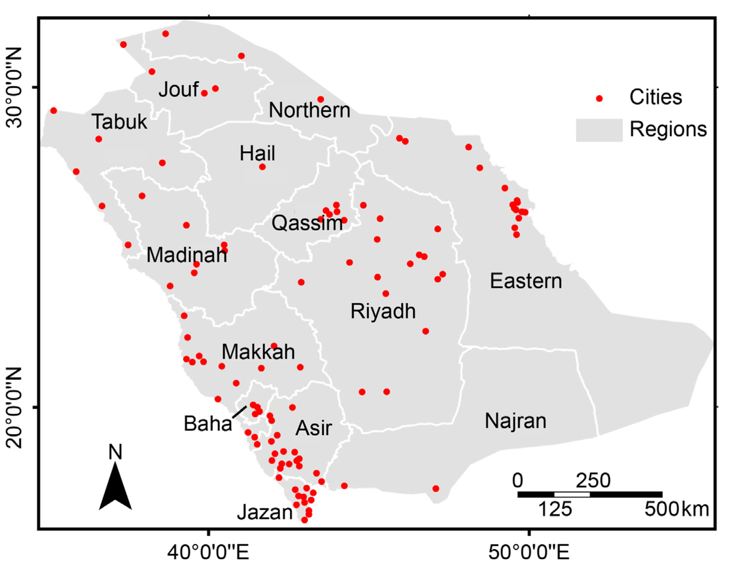
2.1. Cancer, Population and Spatial Data
2.2. Spatial Patterns and Cluster Analyses

- Xi = the crude incidence rate of cancer for the ith city;
- X the mean crude incidence rate of cancer for all of the cities in the study area;
- Xj = the crude incidence rate of cancer for the jth city;
- Wij = a weight parameter for the pair of cities i and j that represents proximity; and
- n = the number of cities.

- Xi = the crude incidence rate of cancer for the ith city;
- X = the mean crude incidence rate of cancer for the cities in the study area;
- Xj = the crude incidence rate for the jth city;
- Wij = a weight parameter for the pair of cities i and j that represents proximity; and
- S = the standard deviation of the crude incidence rate of cancer in the study area.
2.3. Modeling Spatial Relationships


3. Results

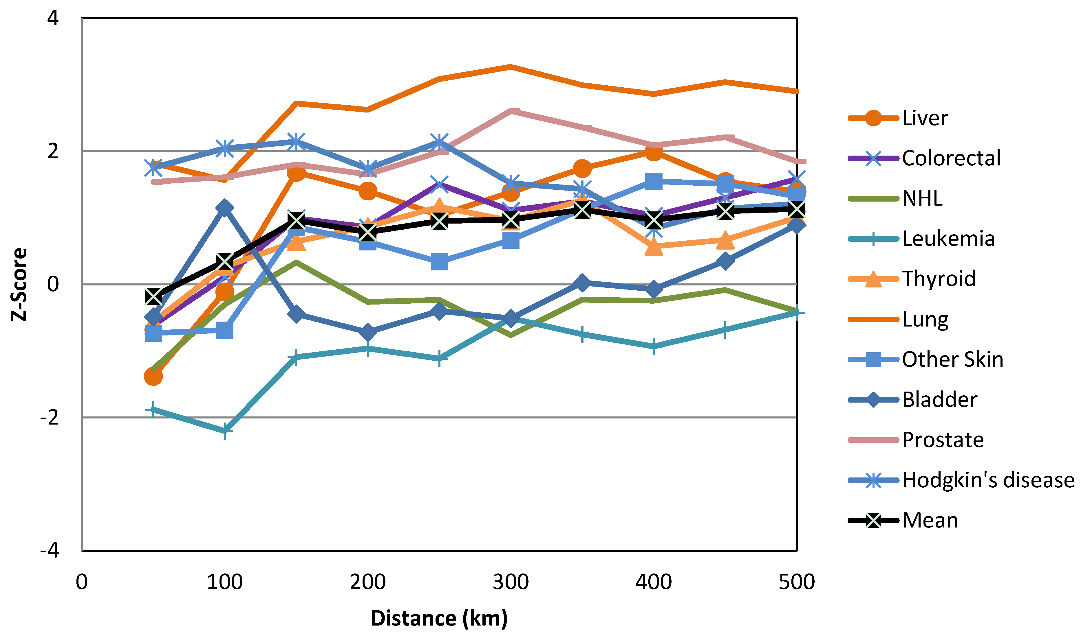
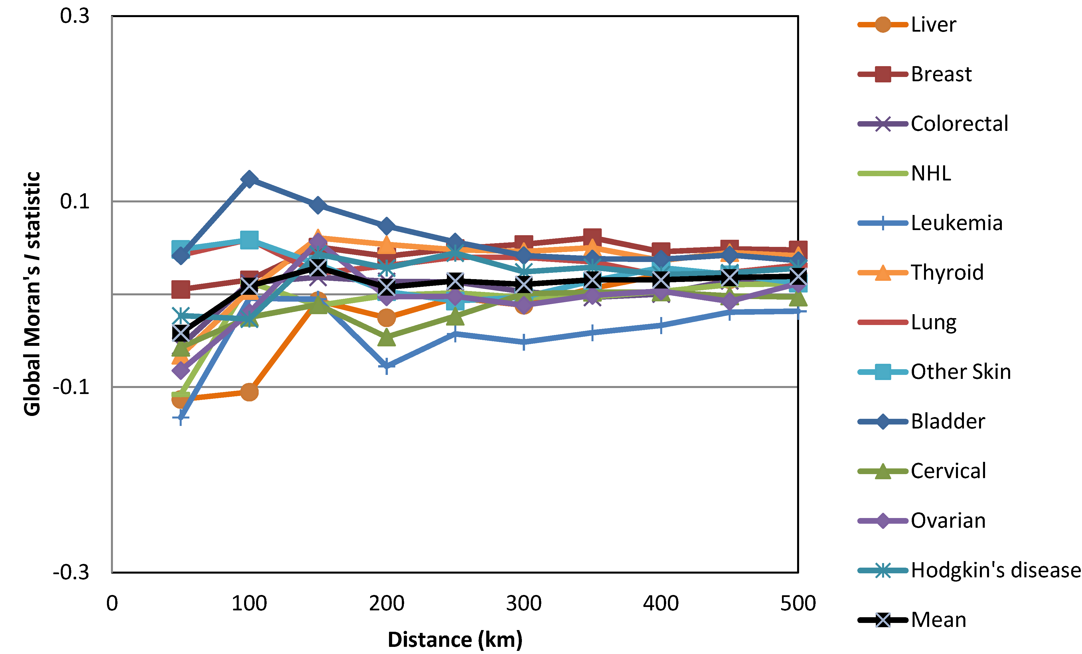
| Cancer Site | All | Male | Female |
|---|---|---|---|
| Breast | 4,668 | 106 | 4,562 |
| NHL | 3,483 | 2,018 | 1,465 |
| Colorectal | 3,322 | 1,763 | 1,559 |
| Leukemia | 3,286 | 1,879 | 1,407 |
| Liver | 2,831 | 2,027 | 804 |
| Thyroid | 2,695 | 595 | 2,100 |
| Lung | 1,867 | 1,464 | 403 |
| Other skin | 1,660 | 957 | 703 |
| Hodgkin’s Disease | 1,616 | 982 | 634 |
| Bladder | 1,425 | 1,122 | 303 |
| Prostate | 1,290 | 1,290 | 0 |
| Ovary | 786 | 0 | 786 |
| Cervix uteri | 641 | 0 | 641 |


| Cancers | Gender | HH | HL | LH | LL | Not Sig. | Regions with HH Clusters | |||||
|---|---|---|---|---|---|---|---|---|---|---|---|---|
| No. | % | No. | % | No. | % | No. | % | No. | % | |||
| Liver | Male | 5 | 4.5 | 3 | 2.7 | 3 | 2.7 | 0 | 0 | 100 | 90.1 | Riyadh, Qassim |
| Female | 1 | 0.9 | 2 | 1.8 | 0 | 0 | 0 | 0 | 108 | 97.3 | Riyadh | |
| Colorectal | Male | 5 | 4.5 | 2 | 1.8 | 1 | 0.9 | 0 | 0 | 103 | 92.8 | Eastern, Qassim, Riyadh |
| Female | 1 | 0.9 | 3 | 2.7 | 0 | 0 | 0 | 0 | 107 | 96.4 | Qassim | |
| NHL | Male | 1 | 0.9 | 5 | 4.5 | 1 | 0.9 | 0 | 0 | 104 | 93.7 | Riyadh |
| Female | 1 | 0.9 | 2 | 1.8 | 0 | 0 | 0 | 0 | 108 | 97.3 | Eastern | |
| Leukemia | Male | 2 | 1.8 | 3 | 2.7 | 0 | 0 | 0 | 0 | 106 | 95.5 | Qassim |
| Female | 0 | 0 | 1 | 0.9 | 0 | 0 | 0 | 0 | 110 | 99.1 | None | |
| Thyroid | Male | 6 | 5.4 | 4 | 3.6 | 0 | 0 | 0 | 0 | 101 | 91 | Eastern, Qassim |
| Female | 9 | 8.1 | 4 | 3.6 | 2 | 1.8 | 0 | 0 | 96 | 86.5 | Riyadh, Eastern | |
| Lung | Male | 7 | 6.3 | 1 | 0.9 | 3 | 2.7 | 0 | 0 | 100 | 90.1 | Eastern |
| Female | 4 | 3.6 | 3 | 2.7 | 0 | 0 | 0 | 0 | 104 | 93.7 | Eastern | |
| Other skin | Male | 4 | 3.6 | 0 | 0 | 0 | 0 | 0 | 0 | 107 | 96.4 | Asir, Jizan, Qassim |
| Female | 2 | 1.8 | 3 | 2.7 | 0 | 0 | 0 | 0 | 106 | 95.5 | Jizan | |
| Bladder | Male | 2 | 1.8 | 2 | 1.8 | 0 | 0 | 0 | 0 | 107 | 96.4 | Asir |
| Female | 9 | 8.1 | 0 | 0 | 0 | 0 | 0 | 0 | 102 | 91.9 | Jizan, Asir | |
| Hodgkin’s disease | Male | 7 | 6.3 | 4 | 3.6 | 1 | 0.9 | 4 | 3.6 | 95 | 85.6 | Eastern, Qassim |
| Female | 6 | 5.4 | 3 | 2.7 | 2 | 1.8 | 0 | 0 | 100 | 90.1 | Eastern, Riyadh | |
| Breast | Female | 5 | 4.5 | 3 | 2.7 | 4 | 3.6 | 0 | 0 | 99 | 89.2 | Eastern |
| Cervical | Female | 5 | 4.5 | 5 | 4.5 | 4 | 3.6 | 0 | 0 | 97 | 87.4 | Eastern |
| Ovarian | Female | 4 | 3.6 | 6 | 5.4 | 4 | 3.6 | 0 | 0 | 97 | 87.4 | Riyadh |
| Prostate | Male | 7 | 6.3 | 2 | 1.8 | 3 | 2.7 | 0 | 0 | 99 | 89.2 | Eastern |

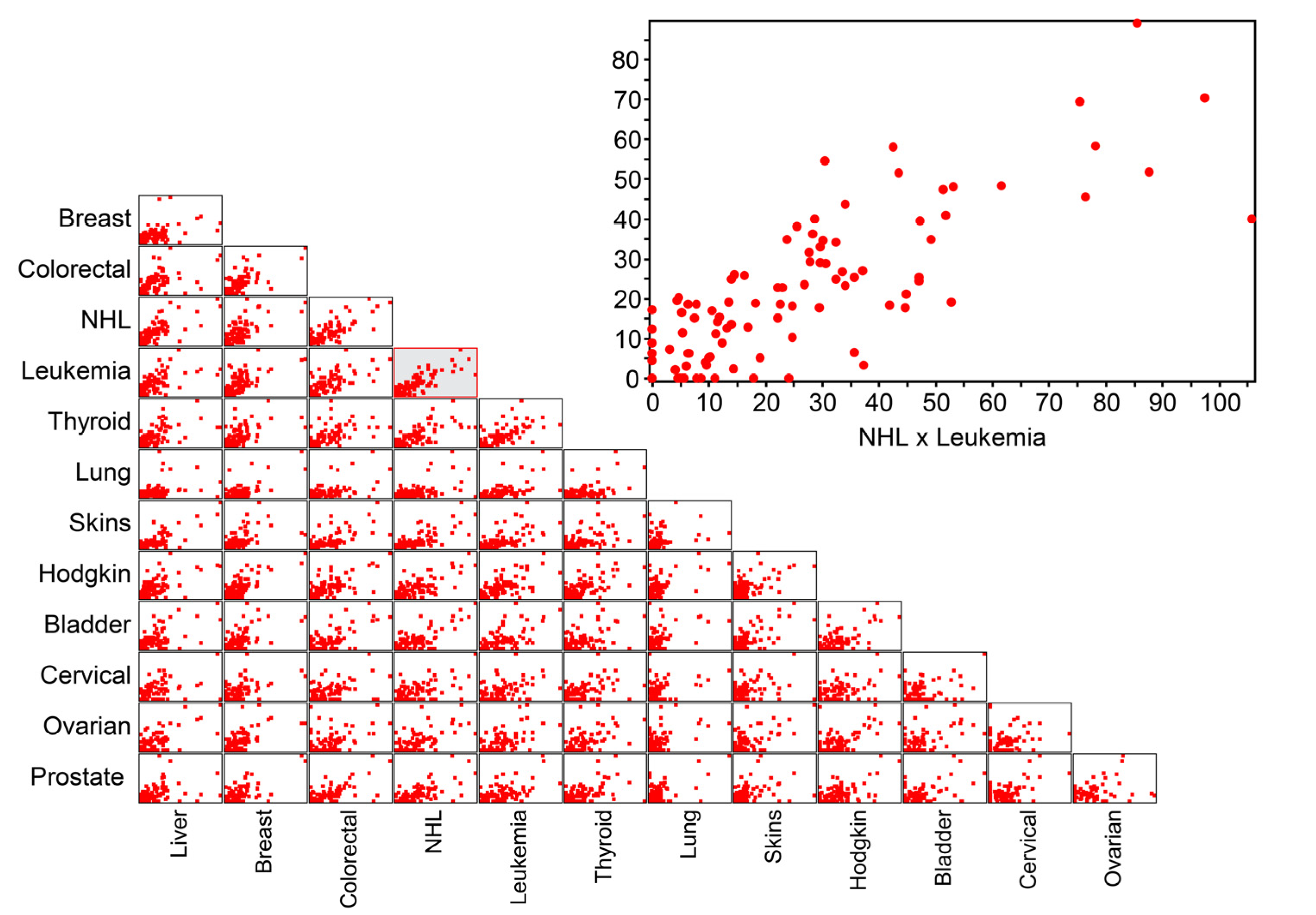
| Cancers | Liver | Breast | Colorectal | NHL | Leukemia | Thyroid | Lung | Other Skin | Bladder | Cervical | Ovarian | Prostate | Hodgkin’s Disease |
|---|---|---|---|---|---|---|---|---|---|---|---|---|---|
| Liver | 1 | ||||||||||||
| Breast | 0.28 * | 1 | |||||||||||
| Colorectal | 0.35 * | 0.52 * | 1 | ||||||||||
| NHL | 0.58 * | 0.51 * | 0.65 * | 1 | |||||||||
| Leukemia | 0.41 * | 0.48 * | 0.51 * | 0.67 * | 1 | ||||||||
| Thyroid | 0.39 * | 0.37 * | 0.35 * | 0.55 * | 0.48 * | 1 | |||||||
| Lung | 0.16 | 0.50 * | 0.32 * | 0.29 * | 0.34 * | 0.31 * | 1 | ||||||
| Other skin | 0.63 * | 0.34 * | 0.49 * | 0.59 * | 0.41 * | 0.32 * | 0.16 | 1 | |||||
| Bladder | 0.35 * | 0.41 * | 0.48 * | 0.58 * | 0.43 * | 0.25 * | 0.29 * | 0.54 * | 1 | ||||
| Cervical | 0.24 * | 0.31 * | 0.30 * | 0.36 * | 0.26 * | 0.29 * | 0.18 | 0.19 | 0.20 | 1 | |||
| Ovarian | 0.49 * | 0.50 * | 0.30 * | 0.46 * | 0.43 * | 0.37 * | 0.28 * | 0.42 * | 0.37 * | 0.09 | 1 | ||
| Prostate | 0.19 | 0.53 * | 0.46 * | 0.48 * | 0.40 * | 0.30 * | 0.35 * | 0.19 | 0.31 * | 0.41 * | 0.20 | 1 | |
| Hodgkin’s disease | 0.43 * | 0.61 * | 0.50 * | 0.53 * | 0.49 * | 0.45 * | 0.38 * | 0.40 * | 0.43 * | 0.31 * | 0.42 * | 0.37 * | 1 |
| Cancers | Liver | Breast | Colorectal | NHL | Leukemia | Thyroid | Lung | Other Skin | Bladder | Cervical | Ovarian | Prostate | Hodgkin’s Disease |
|---|---|---|---|---|---|---|---|---|---|---|---|---|---|
| Liver | 1 | ||||||||||||
| Breast | 0.54 | 1 | |||||||||||
| Colorectal | 0.50 | 0.63 | 1 | ||||||||||
| NHL | 0.74 | 0.58 | 0.66 | 1 | |||||||||
| Leukemia | 0.42 | 0.51 | 0.52 | 0.68 | 1 | ||||||||
| Thyroid | 0.55 | 0.39 | 0.37 | 0.57 | 0.49 | 1 | |||||||
| Lung | 0.52 | 0.56 | 0.34 | 0.46 | 0.61 | 0.47 | 1 | ||||||
| Other skin | 0.70 | 0.75 | 0.77 | 0.72 | 0.58 | 0.57 | 0.74 | 1 | |||||
| Bladder | 0.57 | 0.63 | 0.60 | 0.61 | 0.46 | 0.34 | 0.71 | 0.64 | 1 | ||||
| Cervical | 0.37 | 0.43 | 0.34 | 0.39 | 0.28 | 0.32 | 0.88 | 0.31 | 0.34 | 1 | |||
| Ovarian | 0.50 | 0.74 | 0.47 | 0.58 | 0.49 | 0.53 | 0.73 | 0.63 | 0.59 | 0.20 | 1 | ||
| Prostate | 0.50 | 0.57 | 0.49 | 0.54 | 0.44 | 0.33 | 0.58 | 0.33 | 0.42 | 0.44 | 0.39 | 1 | |
| Hodgkin’s disease | 0.70 | 0.65 | 0.57 | 0.61 | 0.52 | 0.46 | 0.56 | 0.70 | 0.63 | 0.39 | 0.69 | 0.48 | 1 |

4. Discussion
5. Conclusions
Acknowledgments
Conflicts of Interest
References
- Glick, B. The spatial autocorrelation of cancer mortality. Soc. Sci. Med. Med. Geogr. 1979, 13, 123–130. [Google Scholar] [CrossRef]
- Mayer, J.D. The role of spatial analysis and geographic data in the detection of disease causation. Soc. Sci. Med. 1986, 17, 1213–1221. [Google Scholar] [CrossRef]
- Rosenberg, M.S. The bearing correlogram: A new method of analyzing directional spatial autocorrelation. Geogr. Anal. 2000, 32, 267–278. [Google Scholar] [CrossRef]
- La Vecchia, C.; Decarli, A. Correlations between cancer mortality rates from various Italian regions. Tumori 1985, 71, 441–448. [Google Scholar]
- Rosenberg, M.S.; Sokal, R.R.; Oden, N.L.; DiGiovanni, D. Spatial autocorrelation of cancer in western Europe. Eur. J. Epidemiol. 1999, 15, 15–22. [Google Scholar] [CrossRef]
- Boffetta, P.; Castaing, M.; Brennan, P. A geographic correlation study of the incidence of pancreatic and other cancers in Whites. Eur. J. Epidemiol. 2006, 21, 39–46. [Google Scholar] [CrossRef]
- Mandal, R.; St-Hilaire, S.; Kie, J.G.; Derryberry, D. Spatial trends of breast and prostate cancers in the United States between 2000 and 2005. Int. J. Health. Geogr. 2009, 8, 53. [Google Scholar] [CrossRef]
- Struewing, J.P.; Hartge, P.; Wacholder, S.; Baker, S.M.; Berlin, M.; McAdams, M.; Timmerman, M.M.; Brody, L.C.; Tucker, M.A. The risk of cancer associated with specific mutations of BRCA1 and BRCA2 among Ashkenazi Jews. N. Engl. J. Med. 1997, 336, 1401–1408. [Google Scholar] [CrossRef]
- López-Otín, C.; Diamandis, E.P. Breast and prostate cancer: An analysis of common epidemiological, genetic, and biochemical features. Endocr. Rev. 1998, 19, 365–396. [Google Scholar] [CrossRef]
- Valeri, A.; Fournier, G.; Morin, V.; Morin, J.F.; Drelon, E.; Mangin, P.; Teillac, P.; Berthon, P.; Cussenot, O. Early onset and familial predisposition to prostate cancer significantly enhance the probability for breast cancer in first degree relatives. Int. J. Cancer 2000, 86, 883–887. [Google Scholar] [CrossRef]
- Hennekens, C.H.; Buring, J.E. Epidemiology in Medicine; Lippincott Williams & Wilkins: Philadelphia, PA, USA, 1987. [Google Scholar]
- Al-Ahmadi, K.; Al-Zahrani, A.; Al-Dossari, A. A web-based cancer atlas of Saudi Arabia. J. Geogr. Inf. Syst. 2013, 5, 471–485. [Google Scholar]
- Mitchell, A. The ESRI Guide to GIS Analysis, Spatial Measurements and Statistics; ESRI: Redlands, CA, USA, 2005. [Google Scholar]
- Tobler, W.R. A computer movie simulating urban growth in the Detroit region. Econ. Geogr. 1970, 46, 234–240. [Google Scholar] [CrossRef]
- Lloyd, C.D. Nonstationary models for exploring and mapping monthly precipitation in the United Kingdom. Int. J. Climatol. 2010, 30, 390–405. [Google Scholar]
- Kalkhan, M. Spatial Statistics: Geospatial Information Modeling and Thematic Mapping, 1st ed.; CRC: New York, NY, USA, 2011. [Google Scholar]
- Moran, P.A.P. Notes on continuous stochastic phenomena. Biometrika 1950, 37, 17–23. [Google Scholar]
- Geary, R.C. The contiguity ratio and statistical mapping. Inc. Stat. 1954, 5, 115–145. [Google Scholar]
- Fortin, M.; Drapeau, P.; Legendre, P. Spatial autocorrelation and sampling design in plant ecology. Vegetatio 1989, 83, 209–222. [Google Scholar] [CrossRef]
- ESRI. 2012. Available online: http://www.esri.com/ (accessed on 3 December 2012).
- Wong, D.W.S.; Lee, J. Statistical Analysis of Geographic Information with ArcView GIS and ArcGIS; John Wiley & Sons: Hoboken, NJ, USA, 2005. [Google Scholar]
- Anselin, L. Local indicators of spatial association—LISA. Geogr. Anal. 1995, 27, 93–115. [Google Scholar] [CrossRef]
- Bland, J.M.; Altman, D.G. Multiple significance tests: The Bonferroni method. BMJ 1995, 310. [Google Scholar] [CrossRef]
- Fotheringham, S.; Brunsdon, C.; Charlton, M.E. Geographically Weighted Regression: The Analysis of Spatially Varying Relationships; Wiley: Chichester, UK, 2002. [Google Scholar]
- Getis, A.; Ord, J.K. The analysis of spatial association by use of distance statistics. Geogr. Anal. 1992, 24, 189–206. [Google Scholar] [CrossRef]
- Al Tamimi, T.M.; Al-Bar, A.; Al-Suhaimi, S.; Ibrahim, E.; Ibrahim, A.; Wosornu, L.; Gabriel, G.S. Lung cancer in the Eastern region of Saudi Arabia: A population-based study. Ann. Saudi. Med. 1996, 16, 3–11. [Google Scholar]
- World Health Organization. Are the Number of Cancer Cases Increasing or Decreasing in the World? 2008. Available online: http://www.who.int/features/qa/15/en/ (accessed on 25 October 2012).
- Blot, W.J.; Fraumeni, J.F., Jr. Cancers of the Lung and Pleura. In Cancer Epidemiology and Prevention, 2nd ed.; Schottenfeld, D., Fraumeni, J.F., Jr., Eds.; Oxford University Press: New York, NY, USA, 1996; pp. 637–665. [Google Scholar]
- Twigg, L.; Moon, G.; Walker, S. The Smoking Epidemic in England; Health Development Agency: London, UK, 2004. [Google Scholar]
- Howington, J. The first Saudi lung cancer guidelines. Ann. Thorac. Med. 2008, 3, 127. [Google Scholar] [CrossRef]
- Alamoudi, O.S. Lung cancer at a University Hospital in Saudi Arabia: A four-year prospective study of clinical, pathological, radiological, bronchoscopic, and biochemical parameters. Ann. Thorac. Med. 2010, 5, 30–36. [Google Scholar] [CrossRef]
- Al-Turki, K.A.; Al-Baghli, N.A.; Al-Ghamdi, A.J.; El-Zubaier, A.G.; Al-Ghamdi, R.; Alameer, M.M. Prevalence of current smoking in Eastern province, Saudi Arabia. East. Mediterr. Health J. 2010, 16, 671–676. [Google Scholar]
- Beeson, W.L.; Abbey, D.E.; Knutsen, S.F. Long-term concentrations of ambient air pollutants and incident lung cancer in California adults: Results from the AHSMOG study. Adventist Health Study on Smog. Environ. Health Perspect. 1998, 106, 813–823. [Google Scholar] [CrossRef]
- Nyberg, F.; Gustavsson, P.; Järup, L.; Bellander, T.; Berglind, N.; Jakobsson, R.; Pershagen, G. Urban air pollution and lung cancer in Stockholm. Epidemiology 2000, 11, 487–495. [Google Scholar] [CrossRef]
- Nafstad, P.; Haheim, L.L.; Oftedal, B.; Gram, F.; Holme, I.; Hjermann, I.; Leren, P. Lung cancer and air pollution: A 27-year follow up of 16 209 Norwegian men. Thorax 2003, 58, 1071–1076. [Google Scholar] [CrossRef]
- Al-Ahmadi, K.; Al-Zahrani, A. NO2 and cancer incidence in Saudi Arabia. Int. J. Environ. Res. Public Health 2013, 10, 5844–5862. [Google Scholar] [CrossRef]
- Delongchamps, N.B.; Singh, A.; Haas, G.P. The role of prevalence in the diagnosis of prostate cancer. Cancer Control 2006, 13, 158–68. [Google Scholar]
- Al-Otaibi, K.M.; Feehan, M. Incidence of Prostate Cancer in Saudi ARAMCO Institution. In Proceedings of the 11th Saudi Urological Conference, Dhahran, Saudi Arabia, 24–26 February 1998; King Fahd Hospital: Dhahran, Saudi Arabia, 1998. [Google Scholar]
- Mosli, H.A. Prostate cancer in Saudi Arabia in 2002. Saudi. Med. J. 2003, 24, 573–581. [Google Scholar]
- Yoshida, A.; Noguchi, S.; Fukuda, K.; Hirohata, T. Low-dose irradiation to head, neck or chest during infancy as a possible cause of thyroid carcinoma in teen-agers: A matched case control study. Jpn. J. Cancer Res. 1987, 78, 991–994. [Google Scholar]
- Ezaki, H.; Ebihara, S.; Fujimoto, Y.; Iida, F.; Ito, K.; Kuma, K.; Izuo, M.; Makiuchi, M.; Oyamada, H.; Matoba, N.; Yagawa, K. Analysis of thyroid carcinoma based on material registered in Japan during 1977–1986 with special reference to predominance of papillary type. Cancer 1992, 70, 808–814. [Google Scholar] [CrossRef]
- Berg, J.P.; Glattre, E.; Haldorsen, T.; Høstmark, A.T.; Bay, I.G.; Johansen, A.F.; Jellum, E. Long-chain serum fatty acids and risk of thyroid cancer: A population-based case control study in Norway. Cancer Causes Control 1994, 5, 433–439. [Google Scholar] [CrossRef]
- Fraker, D.L. Radiation exposure and other factors that predispose to human thyroid neoplasia. Surg. Clin. North Am. 1995, 75, 365–375. [Google Scholar]
- Memon, A.; Varghese, A.; Suresh, A. Benign thyroid disease and dietary factors in thyroid cancer: A case-control study in Kuwait. Br. J. Cancer 2002, 86, 1745–1750. [Google Scholar] [CrossRef]
- Sakoda, L.C.; Horn-Ross, P.L. Reproductive and menstrual history and papillary thyroid cancer risk: The San Francisco Bay Area thyroid cancer study. Cancer Epidemiol. Biomarkers Prev. 2002, 11, 51–57. [Google Scholar]
- Memon, A.; Darif, M.; Al-Saleh, K.; Suresh, A. Epidemiology of reproductive and hormonal factors in thyroid cancer: Evidence from a case–control study in the Middle East. Int. J. Cancer 2002, 97, 82–89. [Google Scholar] [CrossRef]
- Santamaría-Ulloa, C. The Impact of Pesticide Exposure on Breast Cancer Incidence. Evidence from Costa Rica. Población y Salud en Mesoamerica. 2009, 7. article 1. Available online: http://ccp.ucr.ac.cr/revista/volumenes/7/7-1/7-1-1/7-1-1-ing.pdf (accessed on 11 September 2012).
- Sexton, K.; Callahan, M.A.; Bryan, E.F. Estimating exposure and dose to characterize health risks: The role of human tissue monitoring in exposure assessment. Environ. Health Perspect. 1995, 103, 13–29. [Google Scholar]
- International Agency for Research on Cancer. IARC Monographs on the Evaluation of the Carcinogenic Risk of Chemicals to Humans: Occupational Exposures in Petroleum Refining; IARC: Lyon, France, 1998. [Google Scholar]
- Agency for Toxic Substances and Disease Registry (ATSDR). Toxicological Profile for Total Petroleum Hydrocarbons (TPH); U.S. Department of Health and Human Services, Public Health Service: Atlanta, GA, USA, 1999.
- Clapp, R.W.; Jacobs, M.M.; Loechler, E.L. Environmental and occupational causes of cancer: New evidence 2005–2007. Rev. Environ. Health 2008, 23, 1–37. [Google Scholar] [CrossRef]
- Kirkeleit, J.; Riise, T.; Bratveit, M.; Moen, B.E. Increased risk of acute myelogenous leukemia and multiple myeloma in a historical cohort of upstream petroleum workers exposed to crude oil. Cancer Causes Control 2008, 19, 13–23. [Google Scholar] [CrossRef]
- Zusman, M.; Dubnov, J.; Barchana, M.; Portnov, B.A. Residential proximity to petroleum storage tanks and associated cancer risks: Double Kernel Density approach vs. zonal estimates. Sci. Total Environ. 2012, 441, 265–276. [Google Scholar] [CrossRef]
- Parenteau, M.P.; Sawada, M.C. The modifiable areal unit problem (MAUP) in the relationship between exposure to NO2 and respiratory health. Int. J. Health Geogr. 2011, 10. [Google Scholar] [CrossRef]
- Openshaw, S. The Modifiable Areal Unit Problem; Geo Books: Norwich, UK, 1984. [Google Scholar]
- Cockings, S.; Martin, D. Zone design for environment and health studies using pre-aggregated data. Soc. Sci. Med. 2005, 60, 2729–2742. [Google Scholar] [CrossRef]
- Schuurman, N.; Bell, N.; Dunn, J.R.; Oliver, L. Deprivation indices, population health and geography: An evaluation of the spatial effectiveness of indices at multiple scales. J. Urban Health 2007, 84, 591–603. [Google Scholar] [CrossRef]
- Kloog, I.; Haim, A.; Portnov, B.A. Using kernel density function as an urban analysis tool: Investigating the association between nightlight exposure and the incidence of breast cancer in Haifa, Israel. Comput. Environ. Urban Syst. 2009, 33, 55–63. [Google Scholar] [CrossRef]
© 2013 by the authors; licensee MDPI, Basel, Switzerland. This article is an open access article distributed under the terms and conditions of the Creative Commons Attribution license (http://creativecommons.org/licenses/by/3.0/).
Share and Cite
Al-Ahmadi, K.; Al-Zahrani, A. Spatial Autocorrelation of Cancer Incidence in Saudi Arabia. Int. J. Environ. Res. Public Health 2013, 10, 7207-7228. https://doi.org/10.3390/ijerph10127207
Al-Ahmadi K, Al-Zahrani A. Spatial Autocorrelation of Cancer Incidence in Saudi Arabia. International Journal of Environmental Research and Public Health. 2013; 10(12):7207-7228. https://doi.org/10.3390/ijerph10127207
Chicago/Turabian StyleAl-Ahmadi, Khalid, and Ali Al-Zahrani. 2013. "Spatial Autocorrelation of Cancer Incidence in Saudi Arabia" International Journal of Environmental Research and Public Health 10, no. 12: 7207-7228. https://doi.org/10.3390/ijerph10127207
APA StyleAl-Ahmadi, K., & Al-Zahrani, A. (2013). Spatial Autocorrelation of Cancer Incidence in Saudi Arabia. International Journal of Environmental Research and Public Health, 10(12), 7207-7228. https://doi.org/10.3390/ijerph10127207