Abstract
Granitic residual soils are soils formed by the in situ weathering of intrusive granitic rocks and are present in different parts of the world. Due to their large presence, many civil engineering projects are carried out on and within these soils. Therefore, a correct characterization of the slopes is necessary for slope stability studies. This investigation aims to study the influence of the values of geomechanical parameters (specific weight, cohesion, and friction angle) and the geometry of a slope (height and inclination) on slope stability of residual granitic soils in dry and static conditions. To this end, an automatic system was developed for the numerical study of cases using the finite element method with limit analysis. The system allows modeling, through Monte Carlo simulation and different slope configurations. With this system, the safety factors of 5000 cases were obtained. The results of the models were processed through the SAFE toolbox, performing a Regional Sensitivity Analysis (RSA). The results of this research concluded that the order of influence of the factors were: slope angle > slope height > cohesion > friction angle > unit weight (β > H > c >
> γ).
1. Introduction
Soil mechanics has traditionally been focused on the study of sedimentary soils; however, recently, there has been growing interest in residual soils. Granitic residual soils are a type of residual soil originating from the in situ weathering of granitic intrusive rocks exposed at or near the surface. These types of soils are common in numerous parts of the world. The geotechnical characteristics of residual granitic soils have been studied in Brazil [1,2], China [3,4], Hong Kong [5], Malaysia [6], Portugal [7], South Korea [8], and Thailand [9], to name a few. A granitic residual soil, locally known as “maicillo” is commonly found in Chile. Maicillo is a residual soil resulting from the in situ weathering of granitic rocks formed from intrusive bodies of the Cordillera de la Costa coastal batholith situated parallel to the Pacific coast of Chile. It is one of Chile’s most abundant residual soils and can be found between the Valparaíso Region (33°00′ S) and the Nahuelbuta mountain range, (40°00′ S) [10,11], covering a length of approximately 600 km. Due to the widespread occurrence of this type of soil in Chile and other parts of the world, infrastructure works frequently encounter zones composed of this material, and, therefore, excavations in it are common. Thus, a correct characterization of the materials that make up slopes is necessary for slope stability studies and to guarantee the safety of excavations. The understanding of the influence of each of the factors that determine the stability of a slope in this type of material facilitates its characterization, particularly parameters whose characterizations are much more sensitive. However, the applicability of sophisticated sensitivity analysis methods in geotechnical engineering is normally limited by the amount of available information, both field measurements and information obtained using numerical modeling.
Probabilistic and sensitivity analyses are useful tools for studying slope stability in rocks and soils. Hamm et al. [12] mentioned that slope designers are interested in understanding which factors influence slope failure in order to implement mitigation, maintenance, and repair measures. Therefore, these probabilistic analyses proved to be interesting research topics. Navarro et al. [13] stated that engineers are not completely satisfied with the solutions to given problems provided by traditional approaches, necessitating additional results. They emphasized that, on occasion, knowing the safety factor (SF) or the characterization of the geometry of the failure surface is insufficient. Baker and Leschinsky [14] proposed the inclusion of safety maps as a source of information on parameter changes and how they modify the slope’s safety factor and the resulting failure surface. Meanwhile, Li et al. [15] proposed the inclusion of the influence of human activities on stability.
Sensitivity analysis is a powerful method that can be used to derive information on the influence of different parameters on the stability of a slope. For example, Agam et al. [16] carried out a sensitivity analysis for an unreinforced slope composed of a stratum of residual soil over a sandstone stratum located in Kuala Lumpur, Malaysia. The study used Spencer’s method [17] and the general limit equilibrium method of slices (GLE) to obtain the safety factor associated with variations in cohesion, friction angle, unit weight, and water table position. The authors found the following order of parameter influence: water table position, followed by the residual soil friction angle, cohesion, and unit weight. They also stated that the underlying sandstone stratum parameters did not influence the analysis, as the failure surface did not reach this material.
Aladejare and Akeju [18] used a Monte Carlo simulation to determine the failure probability of a rock slope in Sau Mau Ping, Hong Kong. They employed the model proposed by Hoek [19] and Hoek and Bray [20] to compare the results with those found by other authors for the same location [19,21,22,23,24,25]. Two types of slope stability analyses were performed, one considering the existence of a tension crack, and the other not considering it. In both cases, cohesion, friction angle, tension crack depth, and water column height were modified in order to determine the influence of height on the design of rock slopes. The authors concluded that it is effective to include the variability and uncertainty of rock properties and slope geometry in the design.
Chang et al. [26] and Liang and Sui [27] used the control variable method (CVM) and the orthogonal design method (ODM) to study the influence of freeze-thaw cycles on slope stability in sandstones and dry cohesionless slopes in the Chinese provinces of Xinjiang and Yingpan, respectively. Chang et al. [26] found that safety factor decreased as density, cohesion, and friction angle decreased. The authors concluded that the friction angle presented the highest sensitivity index in their case study. Meanwhile, Liang and Sui [27] used a simplified analytical model with a plane failure surface and concluded that the parameters with the greatest sensitivity index were both friction angle and cohesion.
Xie et al. [28] and Ning et al. [29] implemented the Grey relational method (GRM) [30] combined with the Universal Distinct Element method (UDEM) to determine the factors influencing toppling and bending of layers of rocks inclined perpendicular to the angle of the slope. Xie et al. [28] carried out a theoretical study based on normal parameters, while Ning et al. [29] applied a similar methodology to the study of a slope located on the Yalong River in southeast China. This method requires fewer tests than the orthogonal test method (OTM) and allows the influence of sub-factors on the main factor to be determined. These sub-factors are the geometry, the physical and mechanical parameters of the materials, and the mechanical parameters of the discontinuities or joints.
Hamm et al. [12] applied the combined slope hydrology and stability model (CHASM) to analyze the slope stability of sandy and clayey materials under the influence of the water table position, using cases found in the literature [31,32]. They performed modeling using the limit equilibrium method, specifically Bishop’s method [33]. The soil strength parameters were analyzed using the variance-based sensitivity analysis (VBSA) method of Sobol’s [34] and the replicated Latin hypercube sampling (rLHB) [35]. In the analyzed cases, the authors reported that the parameter with the greatest influence in sandy clay is cohesion, while in sand, it is the friction angle. Xu et al. [36] used the least angle sensibility regression (LASR) [37] and Sobol’s method combined with Monte Carlo simulation to determine the range of input factor values. The authors used the simplified analytical expression for infinite slopes, and stated that LASR presents better performance and that it is not possible to distinguish between sensitivity to slope geometry and soil parameters, with slope inclination being the factor with the highest sensitivity index. Li et al. [15] implemented the sparse polynomial chaos expansion (SPCE) model to quantify uncertainty, combined with the upper bound limit analysis theory and a pseudo-static analysis using a horn-type failure surface. The probabilistic analysis was performed using Monte Carlo simulation, defining the performance function and failure probability. Latin hypercube sampling was used to obtain the cohesion, friction angle, horizontal seismic coefficient, specific weight, slope angle, and width-height ratio parameters required for the 3D model. The parameters with the greatest influence on the safety factor were cohesion and friction angle, with the authors proposing future studies in which anthropogenic effects on slope stability and dynamic activity could be included.
Based on the reviewed literature, it can be highlighted that, in general, geometry is the most influential factor, with slope height and inclination being the factors that produce the greatest safety factor variation. In second place, rock and soil strength parameters (cohesion and friction angle) follow slope geometry in the influence ranking. However, if the model includes them, these parameters are relegated to the mechanical parameters and properties of discontinuities or joints. Finally, parameters such as the specific weight of the material, the Poisson coefficient, or the Young module generally have less influence on slope stability.
Most of the revised studies used either limit equilibrium or finite elements to obtain the data. In soil slope stability analysis, limit equilibrium is used more often, and due to their simplicity, simplified analytic formulations are commonly used along with the slice method. The most frequent failure criteria used are Mohr–Coulomb and Hoek for soils and rocks, respectively.
A large portion of the studies found in the literature on the influence of the value of geomechanical parameters and geometry is limited to the use of unsophisticated analysis tools or the simplification of the problem to enable a quantity of data sufficient to perform the study [12,16,18,24,27,38,39]. In both cases, it cannot be guaranteed that the analysis and its methodology do not influence the results. In this study, along with sensitivity analysis, a methodology is proposed to automatically perform a large number of slope stability simulations, utilizing a geotechnical model composed of the finite element model, along with using limit analysis (FELA) with lower bound and upper bound theorems, the shear strength reduction factor method (SSRM), and the Mohr–Coulomb constitutive model. The usage of a calculation methodology, based on limit analysis, allows the obtainment of maximum and minimum theoretical values of the safety factor of slopes without the need for calculation hypotheses as in limit equilibrium methods or geometric simplifications in the definition of the failure surface such as those performed in analytical methods and limit equilibrium methods. Finally, the influence of each of the studied slope stability parameters were obtained through regional sensitivity analysis (RSA). The modeling was performed for parameter values typically found in the literature for residual granitic soils in order to ascertain the influence of each on the resulting safety factor.
The objective of this investigation is to study the influence of the parameters that characterize both the material and the geometry of a slope on its stability. Dry static conditions for the typical ranges of parameter values of roadworks in residual granitic soils found in Chile were studied. The selected sensitivity analysis method requires a large database to function. However, stability analysis of relatively complex geometries are slow, and usually, the available software does not include a built-in sensitivity analysis tool. If the software does include it, it is limited to elementary analyses. Therefore, a system to obtain large datasets has been designed for the present work. This system uses Monte Carlo simulation to enable the model-building and running process based on the random generation of input variables. It uses a uniform probability distribution in the generation of the variables and allows the value ranges of the geometric and mechanical variables of the material that defines a slope to be specified. While in some studies, it was stated that two of the most important factors for the stability of any slope were the water table height and the seismic effect, these factors have not been included in the present investigation in order to better enable the influence of the study parameters to be obtained.
2. Materials and Methods
To carry out this investigation, two geotechnical constitutive models were used for the finite element simulations. Equal slope, geometry, and soil parameters were simulated using different finite element types based on the upper and lower bound plasticity theorems. To assess the safety factor using finite element simulations, the Shear Strength Reduction Method (SSRM) was used. In these conditions, two safety factors were determined for every simulation, corresponding to each limit theorem.
Traditionally, slope stability analysis has been performed using limit equilibrium methods, generally based on the slice method or expressions devised for simplified geometrical conditions. The methodology employed in the present investigation solves a large part of the problems associated with the use of these methods, as it more realistically represents the geotechnical behavior of slopes. In addition, the finite element limit analysis method does not presuppose the geometry or position of the failure surface and does not require a calculation hypothesis to resolve the static indeterminacy generated in the slice method. To analyze the influence of the geomechanical parameters and the geometry of a slope, once the simulations were performed, regional sensitivity analysis (RSA) was used to determine the area of influence of the input with respect to the outputs corresponding to the safety factor.
2.1. Geotechnical Model
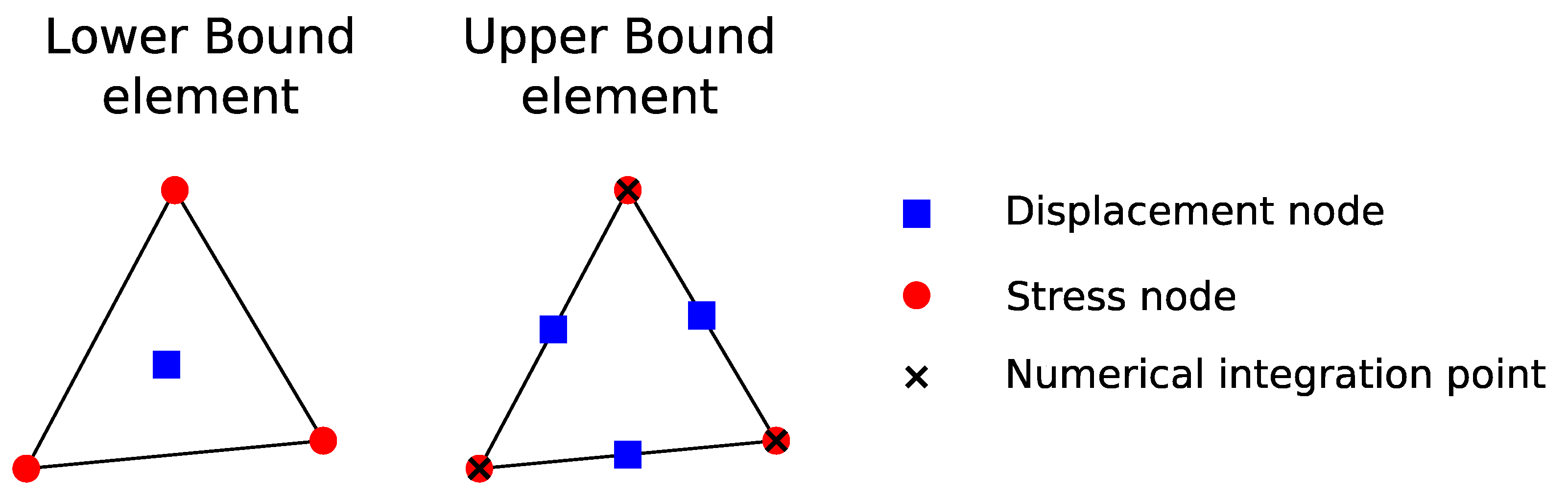
The implementation of lower and upper bound plasticity theorems using finite elements was described by Sloan [40,41]. The limit analysis theorems are employed to determine the maximum and minimum stress that the soil could achieve (according to the stress boundary surface), ensuring than their actual value is within its theoretical range. The theory of plasticity assumes the soil to be a perfectly plastic material. Implementing the lower bound theorem in finite element establishes that the estimation of the lower bound of the actual load limit is given by any statically admissible stress field, where stress discontinuities are only permitted at the interface of the triangular elements of the model. In the software used in this investigation, first-order triangular elements with a linear variation of the stresses between the nodes and a Gauss point are used [42]. Meanwhile, implementing the upper bound theorem in finite elements establishes that the upper bound of the actual load limit can be deduced by comparing the dissipated power of any kinematically admissible velocity field and the power dissipated by external loading, where the displacements between elements are continuous. In this case, triangular elements with six nodes, linear interpolation of stresses, quadratic interpolation of displacements, and three Gauss points are used [42]. Figure 1 shows a diagram of the two types of elements used in this study.
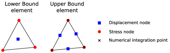
Figure 1.
Triangular element of the finite element model. After [42].
The shear strength reduction method (SSRM) [43] was employed to obtain finite elements’ safety factor values. It represents the same safety factor concept that is typically used in conventional calculations of slopes using analytical or limit equilibrium methods, applying a reduction factor to the strength parameters. The shear strength reduction method is an algorithm used to complement the analysis with finite elements. To perform any finite element analysis, the first step is to discretize the area of study with elements that replace the original geometry in computations. As shown in Figure 1, each of these elements is composed of different types of nodes. Conventional finite element analysis calculates the node displacements, and based on them, the stresses and deformations produced in the elements that constitute the model are determined. To use the finite element method, a constitutive model that allows deformation to be related to stress is necessary. The most typical constitutive model in soil mechanics is the perfect elastoplastic model with the Mohr–Coulomb failure criterion, which is used in this investigation. The shear strength reduction method introduces an equal reduction factor to the strength parameters and searches for the maximum value it can have for the model to remain stable. This parameter’s maximum value is the analyzed slope’s strength reduction factor (SRF). In its most typical form, the Mohr–Coulomb criterion uses a linear envelope, such that the parameters that define it, called strength parameters, are cohesion (c) and friction angle (ϕ). The maximum shear stress (τ) as a function of the effective normal stress (σ’) can be obtained using the linear Mohr–Coulomb failure envelope, which is defined using Equation (1).
Slope stability is usually analyzed by introducing a material safety factor (SF), that is, the value by which the value of the strength parameters can be reduced until a strict equilibrium is reached. To this end, the available shear stress is calculated using Equation (2).
When the finite element method is used, the instability situation is reached through the iterative reduction of strength parameters via a strength reduction factor (SRF), which divides the soil strength parameters, resulting in a new value of the strength parameters used in the calculation. This process is carried out until it induces a slope collapse. Final shear strength parameters are determined as the lowest values that produce a stable model, and the failure surface as the area in the model in which the maximum shear strain is produced. Therefore, the safety factor (SF) and the strength reduction factor (SRF) are analogous concepts that can be used interchangeably. Based on the foregoing, both the SF and SRF can be defined as the ratio of the initial Mohr–Coulomb strength parameters to the minimum value of the parameters that produce a stable model or the ratio of initial soil strength to the strength at failure [44]. Equations (3)–(5) show the mathematical expressions of cohesion, friction angle, and the safety factor, respectively.
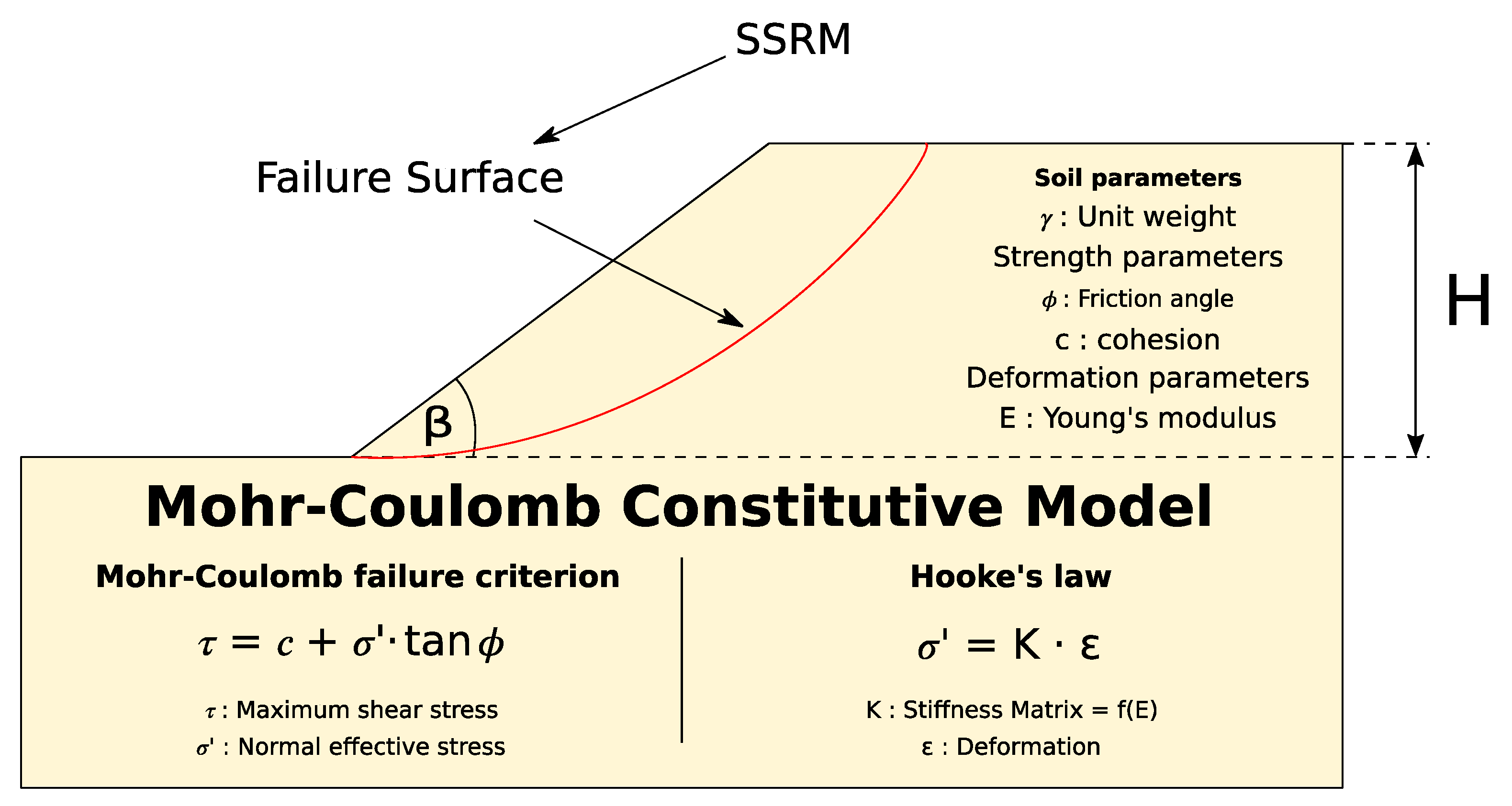
Lu et al. [45] and Li et al. [15] stated that limit equilibrium methods (LEM) are used more than finite element methods; however, the latter considered stresses and deformations in the model. Finite element methods (FEM) provide SF estimates that are slightly lower than those obtained using limit equilibrium methods ([46,47,48,49,50,51,52] in [53]), and their computational costs are higher [54]. Among the main advantages of FEM compared to other methods is that a slope failure surface is not assumed, and hypotheses to solve static indeterminacy that result from the slice division typically used in limit equilibrium methods for complex geometries are not needed, improving calculation precision [15,45,53,55]. Therefore, as this study aims to determine the influence of the geomechanical parameters of granitic residual soil and slope geometry on the overall safety factor for slope stability, the finite element method using the shear strength reduction method was selected as the analysis method for the geotechnical model. Figure 2 presents a conceptual diagram of the geotechnical model described.
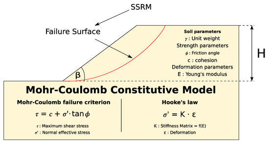
Figure 2.
Conceptual diagram of the geotechnical model of a slope.
2.2. Sensitivity Analysis
Sensitivity analysis methods allow the determination of how the variation of an output factor can be affected by the variation of the values of input factors or parameters of a numerical model [56]. Pianosi et al. [56] described three elements present in sensitivity analysis methods: model, input factor(s), and output factor(s). A model is a mathematical procedure that simulates the behavior of a given system. Inputs are parameters, variables, and boundary conditions of the model, while outputs are the elements obtained after running the model. Scalar functions can be derived from the outputs (Equation (6)); they can be objective functions (performance calculated as the comparison of a model with observations) or prediction functions (scalar functions that represent a specific place or time).
Sensitivity analyses can be classified according to various criteria: variability (local or global), approach (quantitative or qualitative), sampling strategy (one at a time or all at once), and objective (screening, ranking, or mapping), such that an analysis method must be adopted in accordance with the objective of the investigation. Thus, to determine the influence of geomechanical parameters and slope geometry on the safety factor, it must be ascertained which input factors have the greatest influence on the output factor (ranking) and in which variability space the influence occurs (mapping).
According to the classification carried out by Pianossi et al. [56], among the sensitivity analysis methods with the aforementioned characteristics are regional sensitivity analysis (RSA), correlation and regression methods, variance-based sensitivity analysis (VBSA), and density-based sensitivity analysis (DBSA). The regional sensitivity analysis (RSA) method allows the identification of regions in the input space associated with particular output values and permits mapping and ranking. Correlation and regression methods allow information on output sensitivity to be obtained by performing ranking or mapping, but not both at the same time. Due to their characteristics, variance-based methods (VBSA) allow screening and ranking based on the variance of output distributions. Methods based on density (DBSA) also allow screening and ranking, but unlike VBSA, they perform these tasks on the basis of variation of the probability density function (PDF) of the outputs.
The regional sensitivity analysis method (RSA) [57,58] allows regions of the input space associated with particular output values to be identified. Pianosi et al. [56] added the classification of behavioral models (BM) and non-behavioral models (N-BM), differentiating them in accordance with a threshold or value defined for a previously defined performance measure or prediction function. The results of both groups can be graphed, and, via visual inspection of the cumulative distribution functions, spaces of each parameter that allow sensitivity to be determined or spaces with a positive or negative influence on outputs can be identified. Similarly, the difference between the cumulative distribution functions (CDF) of BM and N-BM measured by the Kolmogorov–Smirnov statistic is used as a measure or index of sensitivity of the model outputs to variations of the analyzed parameter (Equation (7)).
where and are the empirical cumulative distribution functions of the behavioral and non-behavioral input samples. This parameter is also known as the maximum vertical distance (mvd). These empirical functions provide a robust approximation of the underlying distribution, as in the case in which parameterizations are limited to sub-regions of the space.
On the other hand, the relative sensitivity index is defined in Equation (8), where is the sensitivity index of ith parameter and n is the number of total parameters.
2.3. Experimental Design
Numerical simulations were carried out using the previously described geotechnical model. Two input groups can be considered in this model, grouped according to soil and slope geometry properties. Among the soil factors are strength parameters—cohesion (c) and friction angle (ϕ), and the soil state parameters—unit weight, γ The geometry factors are slope height (H) and slope angle (β).
To perform a regional sensitivity analysis (RSA), Pianosi et al. [56] suggested a number of simulations between 100 × M and 1000 × M, where M is the number of model inputs. This study includes five input factors (cohesion, friction angle, unit weight, slope height, and slope angle). First, 1000 simulations were carried out, and the convergence of the results was studied; however, as no convergence was observed, the number of simulations was increased to 5000. Convergence of the results was verified for 5000 simulations; therefore, these simulations were used for all the analyses. The model simulation was carried out through Monte Carlo simulations, assuming for each input parameter the ranges presented in Table 1, which correspond to the typical values of the different parameters for the studied soil type found in the literature. Parameter values were generated assuming that they are independent and with a uniform probability distribution for all parameters used.

Table 1.
Range of model parameters’ variation, assuming a uniform probability distribution.
Slope height depends on the project; it is defined in the slope design and limited by the design requirements, the technical equipment available for construction, and the project budget. Thus, slopes with various heights can be found. In this study, the analyzed slope height range was limited to between 2 and 30 m. According to Chilean regulations for highway slope construction [59], slopes must have a maximum inclination between 26° and 56°; however, Wesley [60] stated that residual soil slopes can be stable even at 60°. Therefore, the slope inclination range for the present analysis was defined as between 26° and 80° in order to include cases of instability in the analysis and simulations. Flandes [61], Viana da Fonseca [62], and Au [63] characterized and described residual granitic soils in Chile, Portugal, and Hong Kong, respectively. Based on these studies, soil strength parameters range from 0 to 5 kPa for the cohesion values of this type of soil and the friction angle varies between 29.5° and 38.0°. It bears mentioning that there are cohesion results greater than 5 kPa in the works of other authors (such as [62,64]). Chilean maicillo is normally classified as silty sand according to the Unified Soil Classification System (ASTM D2487-17). Thus, greater cohesion values are considered excessive, as they could correspond to a granitic residual soil with a greater degree of weathering than the studied material. Based on the work of Rodríguez [64], in which a geomechanical characterization of the granitic residual soil of the Cordillera de Nahuelbuta range in Chile was carried out, a range of 17 to 21 kN/m3 was defined for the unit weight.
The shear strength reduction method (SSRM) was implemented in the finite element-based geotechnical calculation software OptumG2 2021® (Optum Computational Engineering, Copenhagen, Denmark). This program allows the geometric and geomechanical conditions of the slope to be modified and its files to be executed based on external programming codes. To this end, a code in the Python programming language (https://www.python.org, accessed on 19 January 2022) was developed, allowing Monte Carlo simulations to be configured, run, and the obtained results to be saved. The processing of the results was carried out using the SAFE (Sensitivity Analysis For Everybody) Toolbox published by Pianosi et al. [65] in its Python version. This tool allows regional sensitivity analysis (RSA) to be performed, and the results of the ranking and mapping to be represented graphically.
To classify the models as behavioral (BM) and non-behavioral (N-BM), safety factors less than or equal to 1.2 and greater than or equal to 1.2 were used as a prediction measure in the analysis. Results for the safety factor (SF) less than 1.2 are associated with a slope that is unstable and therefore, prone to failure, while simulations with SF ≥ 1.2 are considered stable [53]. The safety factor value necessary to consider the slope stable depends on the project conditions and the regulations employed.
2.4. Generation of Simulations
The use of the sensitivity analysis method requires a large amount of data. In the case of this study, each of the points used in the analysis is the result of a numerical simulation using values in the ranges established by the Monte Carlo simulation as input parameters. Therefore, in this study, 5000 numerical simulations of slopes with different characteristics were generated and analyzed. A system that allows the creation of models and extraction of the results to be automated was used to obtain the results, making the project feasible. The methodology used to generate the models to be studied was implemented in Jupyter Notebooks (https://jupyter.org, accessed on 19 January 2022) using the Python kernel, which allows a well-structured and replicable workflow and simplifies the interaction between the user and the developed software due to the internal organization of the notebook, consisting of cells that can be run independently to have access to partial results in a simple manner. The files produced natively by the program used for modeling (OptumG2), although they have the extension g2x, they are, in reality, files that use the standard extensible markup language (XML), such that they are simple to manipulate using external tools. A “g2x” file is generated for each of the simulations that will be run using the Jupyter notebook and executed using the OptumG2 calculation engine, and the results are extracted from the model output file. Each of the files is generated automatically with upper and lower bound analyses and the desired input parameter values.
Soil parameter values can be incorporated in the OptumG2 file by replacing their value directly with minor changes in the template file. However, the modification of the slope geometry, height, and inclination requires the modification of the geometry of the model. To this end, an initial slope formed by six nodes was used as a template geometry. The positions of nodes 1, 2, 5, and 6 are maintained in the different model executions, while the x and y coordinates of node 4 and only the y coordinate of node 3 vary. With this variation, the slope inclination and height required by each model generated using the Monte Carlo method are obtained. In Figure 3, a diagram of the model modification is shown.
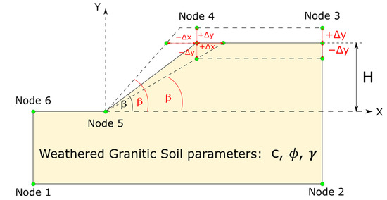
Figure 3.
Slope model template diagram.
The workflow for model creation and calculation is divided into five stages. The first consists of importing the Python libraries necessary for the code to function, both to perform mathematical operations, read, and modify OptumG2 files. Next are the cells used to define the variables that will modify the geometry (height and inclination angle) and soil strength parameters (cohesion, friction angle, and specific weight), the IDs of the nodes on which the slope geometry depends, and the ID of the material of which the slope is composed. The system allows the target intervals for each parameter to be defined and generates random data using a uniform distribution of each parameter. In this phase, a list for each input and the number of elements equal to the number of simulations to be run are obtained. The third stage consists of the modification of the template and the generation of files for calculation. The soil strength parameters and specific weight values are assigned based on the material ID. The process of modifying the geometry and behavior model parameters is carried out iteratively, with a number of cycles equal to the number of simulations (n). The system generates a file with the model of each of the cases to be analyzed. The following stage consists of the execution of the new models, for which the OptumG2 calculation engine is used, accessed via the command line automatically from the notebook. The solution of the modeling is stored in the same files used for the calculation. In the fifth and final stage, the results of each of the executed models, that is, the SF corresponding to the lower and upper bounds, are retrieved. Finally, Comma Separated Values (CSV) files with both input values and the resulting output values are generated for analysis using the SAFE (Sensitivity Analysis For Everybody) Toolbox [65] in its Python version.
3. Results
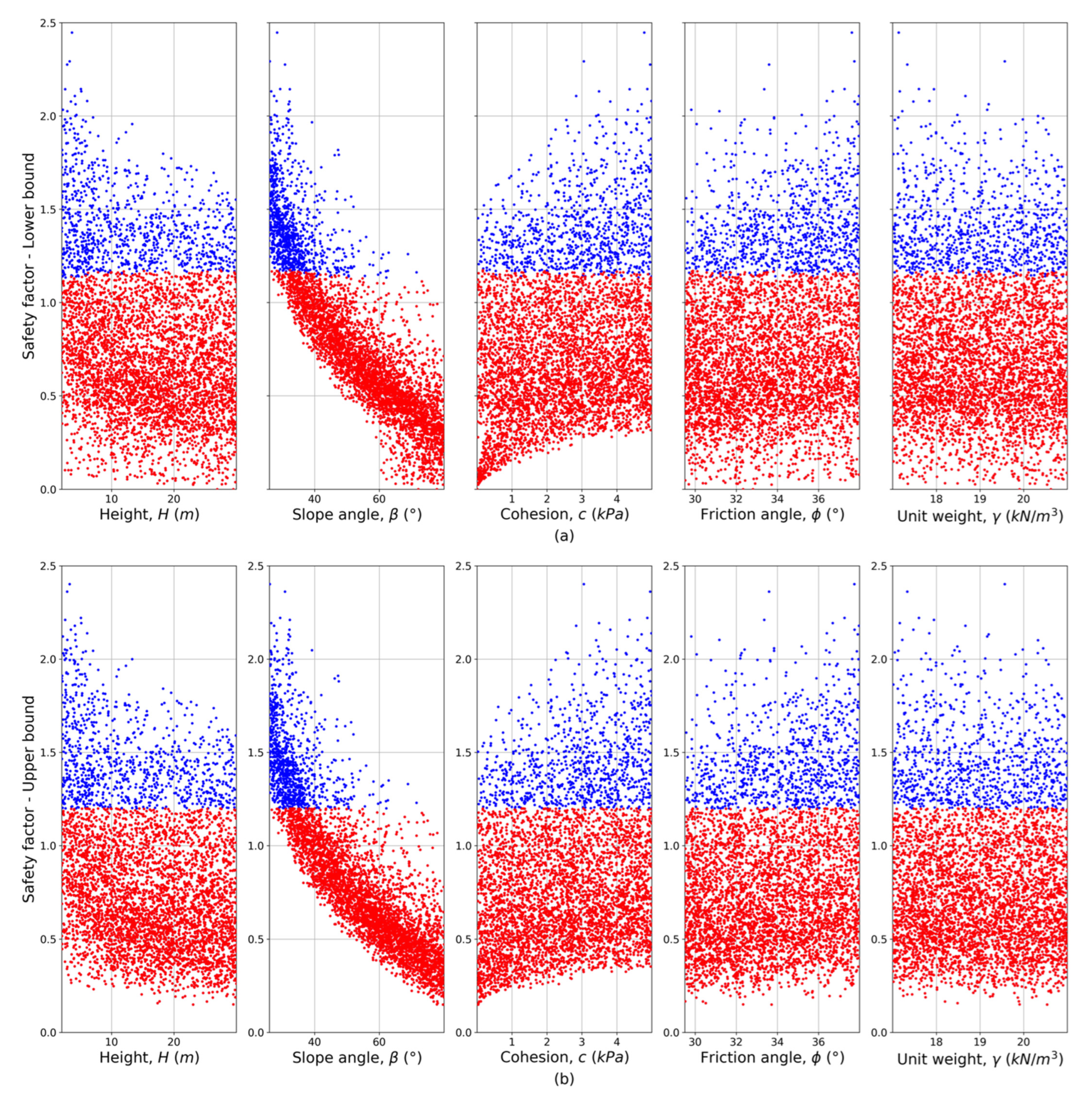
Figure 4 presents the scatter plots of the lower bound (SF-LB) and upper bound (SF-UB) safety factors. Similar behavior is observed in both cases. Behavioral models (BM) are mainly observed when the inclination angle (β) is less than 50°. In the case of slope height (H), BM are observed along all the ranges studied; however, the number of BM increases with lower H values. In the case of cohesion (c) and friction angle (), BM are associated with high c and values. Meanwhile, safety factor sensitivity to unit weight (γ) is not observed.
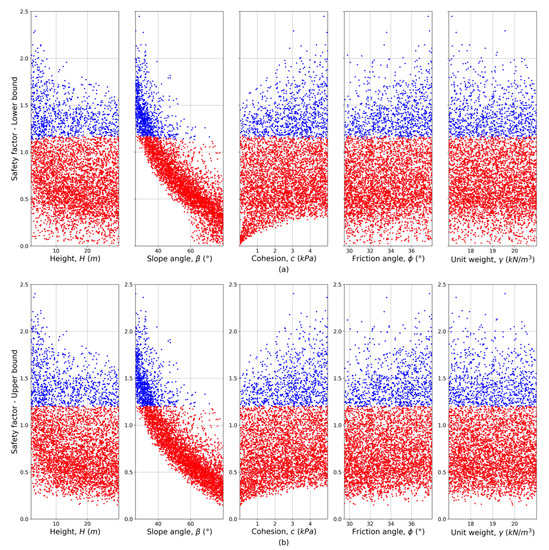
Figure 4.
Scatter plots of the SF as a function of each analyzed parameter for the lower bound (SF-LB) (a) and upper bound (SF-UB) (b). Blue dots represent behavioral models (BM) and red dots non-behavioral models (N-BM).
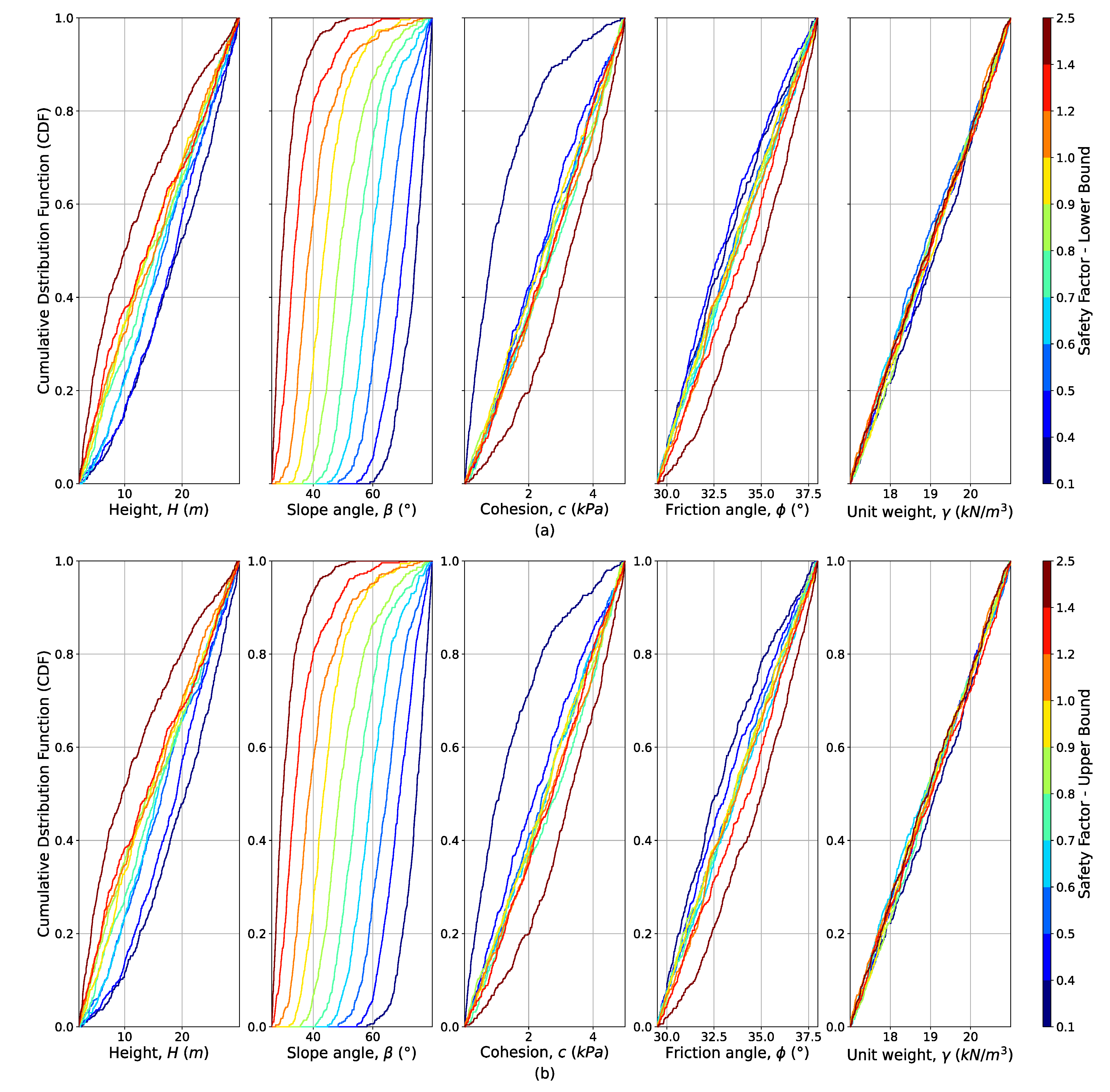
The representation of both lower bound and upper bound safety factors in Figure 4 shows similar distributions for each parameter on the two datasets. Figure 5 presents the cumulative distribution functions (CDF) for SF-LB and SF-UB, grouped into deciles from the most stable 10% of the models (greater SF, brown) to the least stable 10% of the models (lower SF, blue). It is observed that the most stable 10% of the models () are clustered at lower height values (H) and, in general, at H < 10 m (P50 = 10 m). In contrast, the least stable 10% of the models are concentrated above 10 m. Although SF-LB and SF-UB decrease as H increases, stable models () can be obtained when H > 20 m (P90 = 20 m). Regarding slope angle (), it is observed that the lower the slope inclination angle, the greater the SF, with the most stable 10% of the models (SF > 1.4) concentrated at (P90). Meanwhile, the least stable 10% of the models occur over 53°. It is also noted that SF-LB and SF-UB increase when cohesion is greater than 2 kPa (), with the most stable 10% of the models () concentrated above that value. Alternatively, the least stable 10% of the models are clustered at values of (P80). For the friction angle (), the most stable 10% of the models () are concentrated above 31.6° (), while the least stable 10% of the models are obtained for . The unit weight does not present a particular concentration of models for each group.
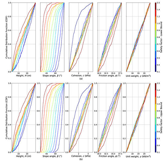
Figure 5.
Cumulative distribution function by deciles of model behavior for (a) lower bound (SF-LB) and (b) upper bound (SF-UB).
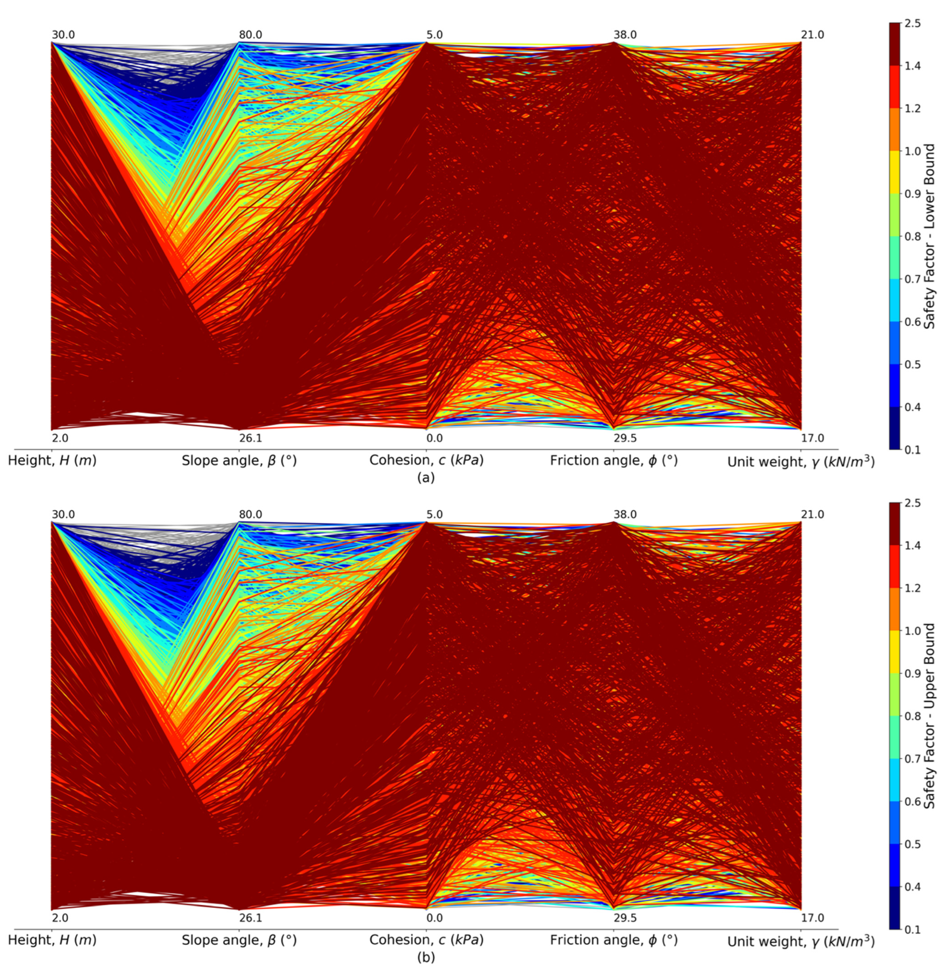
Figure 6 presents a parallel coordinates plot for the lower bound and upper bound SF, grouped by deciles from the most stable 10% of the models (greater SF, brown) to the least stable 10% (lower SF, blue). This plot indicates how the variable values are related to each other according to the performance of the analyzed models. As with the CDF, the SF-LB and SF-UB parallel coordinates plots are similar. Regarding the most stable 10% of the models (SF-LB and SF-UB > 1.4), parameter behaviors are identified. First, stable models are observed throughout the range of H variability (0–30 m), associated mostly with values lower than 39.5. However, it is also possible to find models among the most stable 10% in the range of 39.5 to 53 and a small number between 53 and 66.5. This behavior is attributed to cohesion, friction angle, and unit weight, as a concentration of models is observed when , , and . Meanwhile, another group of stable models is observed for slopes with , , and .
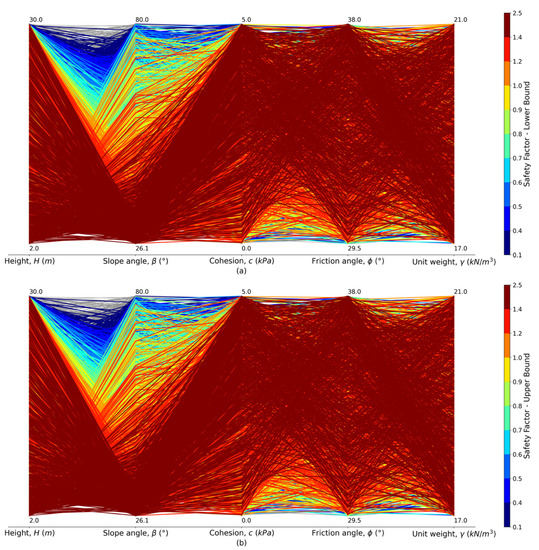
Figure 6.
Parallel coordinates plot for (a) lower bound (SF-LB) and (b) upper bound (SF-UB) safety factors.
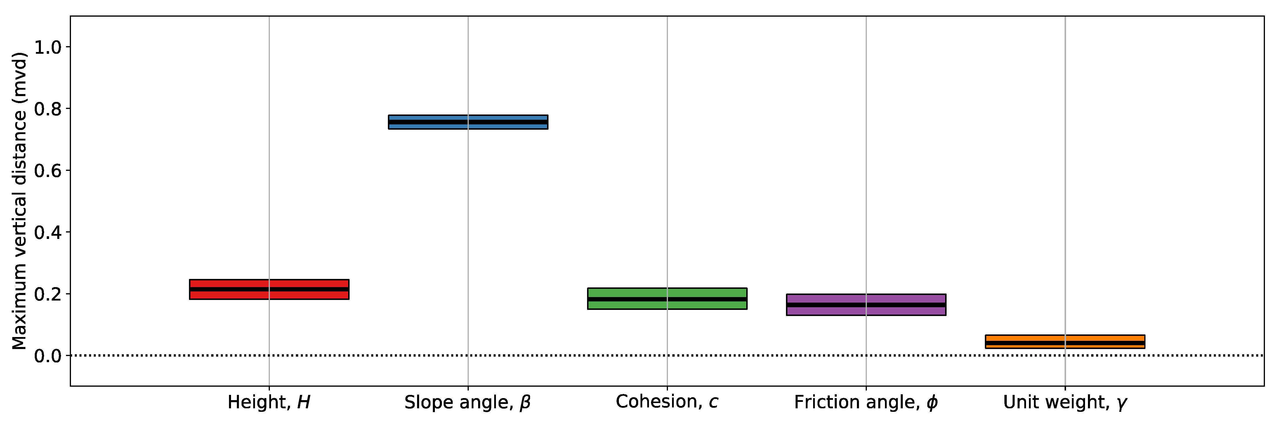
Figure 7 presents the boxplots of the sensitivity index calculated for each factor. In addition, the median of the sensitivity index (SI) and the relative sensitivity index (RSI). In this case, the sensitivity index (SI) corresponds with the maximum vertical distance (mvd), obtained as the maximum difference between the cumulative distribution curves of well-behaved and non-well-behaved models, as defined in Equation (7). On the other hand, the relative sensitivity index was defined in Equation (8). The values of the sensitivity index and the relative sensitivity index are presented in Table 2.
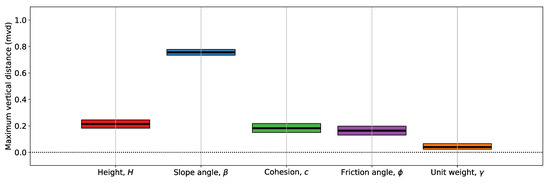
Figure 7.
Boxplot of the sensitivity index for each variable.
Table 2.
Values of the sensitivity index and relative index of each variable.
In accordance, the order of influence of each of the variables on SF-LB and SF-UB is: . Both SF present high sensitivity to , decreasing as this parameter increases. H, c, and have a smaller influence than , with the SF increasing as c and increase, while the SF decrease when H increases. Based on these results, it can be stated that the geometric attributes of a slope are the variables that most influence its stability within the parameter value ranges characteristic of residual granitic soils, followed by soil strength parameters and then its geomechanical properties. However, this statement is limited to the scope of the study, as the effects of rain or hereditary structures are not considered.
4. Discussion
Wesley [66] mentioned that residual soil slopes with inclinations over 45° are not infrequent; however, the author did not differentiate between the different types of residual soils. Results shown in Figure 5 and Figure 6, where it is observed that the most stable 10% of the models are concentrated in a range between 26° and 53°, can corroborate the statement from Wesley [66] regarding residual granitic soils. The author also mentioned that cohesion plays an important role in stability, as shear strength depends on this parameter. The present study results are consistent with Wesley’s conclusions [66], only if the Mohr–Coulomb strength parameters are analyzed, as, in accordance with the sensitivity order, cohesion is third in influence on the SF. It bears mentioning that the works of Flandes [61], Viana da Fonseca [62], and Rodríguez [64] presented different cohesions, which are directly related to the degree of weathering of the material. The degree of weathering was not included in this study; therefore, its analysis may or may not represent the influence of cohesion on the SF, according to Wesley [66].
Siddque and Pradham [53] mentioned a “metastable” state when SF = 1. The authors stated that in this condition, slopes are stable but could fail in conditions of intense rain or due to seismic activity. In addition, Wesley [66] explained that landslides in residual soils occur under intense rainfall, as the increase in pore pressure reduces the effective stress and, therefore, the shear strength of the soil. The author also mentioned that landslides can be triggered by earthquakes. This metastable state is represented in Figure 5 and Figure 6 in orange (1 < SF-LB < 1.1; 1 < SF-UB < 1.2). In Figure 6, it is observed that the metastable models occur at higher slope inclination angles than in the case of the most stable 10% of the models, that is, even with near 70. These models are associated mainly with small heights (H < 7.5 m) and cohesions around 5 kPa. This consideration is important since these slopes can be stable before excavation in dry and static conditions but can easily become unstable after heavy rains or seismic activity.
Li et al. [15] mentioned that slope failure probability depends not only on geomechanical parameters but also on slope geometry. While the case studies of Liang and Sui [27], Xie et al. [28], and Ning et al. [29] did not consider the same materials, geometry, and pore pressure conditions as this study, similarities in the results were found. Liang and Sui [27] also found that geometry factors have the most influence on slope stability; however, they determined that slope height (H) has a greater influence than slope angle () on SF. As in this study, Xie et al. [28] and Ning et al. [29] found that factors associated with geometry have a greater sensitivity index than soil geomechanical parameters but in rock slopes. Likewise, this study presents a ranking that places geomechanical parameters below slope geometry, even though the cohesion sensitivity differs from the results of Hamm et al. [12]. In the case of these authors, for sandy clays, cohesion presented the greatest influence, while in the case of sands, friction angle did; however, in the present study, a granitic residual soil is analyzed, classified by Au [63] as silty sand, for which it could be expected that the friction angle would have a greater influence than cohesion on SF.
5. Conclusions
In most cases, the use of sophisticated sensitivity analysis systems in geotechnical engineering is conditioned by limited data availability. One way of obtaining data is the use of numerical simulations, however, manual generation of these data requires much preparation time. In this study, a system that allows this process to be automated and results to be generated by using Monte Carlo simulations for the ranges of the geometric and soil parameter values that define a slope was developed. The system was used to build a dataset with the results of 5000 simulations, which allowed the use of regional sensitivity analysis (RSA) to study the relative influence of each of the analyzed parameters on the stability of a slope. The data were generated by using value ranges reported in the literature for residual granitic soils.
Limit equilibrium analysis is faster than traditional finite element calculations and produces similar results in terms of safety factors, with a minimal difference between lower and upper bound values for the analyzed slopes. Furthermore, all 5000 simulations were carried out without errors, even though their parameters were randomly obtained within given value ranges, and data extraction from the models was simple by using a Jupyter notebook.
Based on scatter plots and cumulative distribution curve graphs, it can be observed that the safety factors of the lower bound and upper bound models converge at similar values, limiting the overall safety factor range of the slope. Therefore, it can be concluded that within the slope parameter values studied in the present work, the calculated safety factors are influenced mainly by slope geometry and, to a lesser extent, by soil geomechanical parameters. The order of influence of the factors obtained in this study were slope angle > slope height > cohesion > friction angle > unit weight ().
Author Contributions
Conceptualization, E.M., P.L.-M., J.M.M.-C. and R.W.K.; Data curation, M.F.B.-Z.; Formal analysis, M.F.B.-Z. and E.M.; Funding acquisition, E.M.; Investigation, M.F.B.-Z., E.M. and P.L.-M.; Methodology, M.F.B.-Z., E.M. and P.L.-M.; Project administration, P.L.-M., J.M.M.-C. and R.W.K.; Resources, P.L.-M., J.M.M.-C. and R.W.K.; Software, M.F.B.-Z. and P.L.-M.; Supervision, E.M., P.L.-M., J.M.M.-C. and R.W.K.; Validation, E.M., P.L.-M., J.M.M.-C. and R.W.K.; Visualization, M.F.B.-Z., E.M. and P.L.-M.; Writing—original draft, M.F.B.-Z., E.M. and P.L.-M.; Writing—review and editing, E.M., P.L.-M., J.M.M.-C. and R.W.K. All authors have read and agreed to the published version of the manuscript.
Funding
This research was funded by CIBAS 2019-01 Project.
Institutional Review Board Statement
Not applicable.
Informed Consent Statement
Not applicable.
Data Availability Statement
The data presented in this study are available upon request from the corresponding authors. The code developed to perform simulations is available in a public repository under MIT license (https://github.com/MBravo-Zapata/sa_maicillo, accessed on 19 May 2022).
Acknowledgments
The authors would like to acknowledge the postgraduate program of the Faculty of Engineering of the Universidad Católica de la Santísima Concepción during the studies of Matías F. Bravo-Zapata.
Conflicts of Interest
The authors declare no conflict of interest.
References
- Townsend, F.C. Geotechnical Characteristics of Residual Soils. J. Geotech. Eng. 1985, 111, 77–94. [Google Scholar] [CrossRef]
- Coutinho, R.Q.; Silva, M.M.; dos Santos, A.N.; Lacerda, W.A. Geotechnical Characterization and Failure Mechanism of Landslide in Granite Residual Soil. J. Geotech. Geoenviron. Eng. 2019, 145, 05019004. [Google Scholar] [CrossRef]
- Niu, X.; Xie, H.; Sun, Y.; Yao, Y. Basic Physical Properties and Mechanical Behavior of Compacted Weathered Granite Soils. Int. J. Geomech. 2017, 17, 04017082. [Google Scholar] [CrossRef]
- Liu, X.; Zhang, X.; Kong, L.; Chen, C.; Wang, G. Mechanical Response of Granite Residual Soil Subjected to Impact Loading. Int. J. Geomech. 2021, 21, 04021092. [Google Scholar] [CrossRef]
- Wang, Y.-H.; Yan, W. Laboratory Studies of Two Common Saprolitic Soils in Hong Kong. J. Geotech. Geoenviron. Eng. 2006, 132, 923–930. [Google Scholar] [CrossRef]
- Salih, A. Review on Granitic Residual Soils’ Geotechnical Properties. Electron. J. Geotech. Eng. 2012, 17, 2645–2658. [Google Scholar]
- Viana Da Fonseca, A.; Carvalho, J.; Ferreira, C.; Santos, J.; Almeida, F.; Pereira, E.; Feliciano, J.; Grade, J.; Oliveira, A. Characterization of a Profile of Residual Soil from Granite Combining Geological, Geophysical and Mechanical Testing Techniques. Geotech. Geol. Eng. 2006, 24, 1307–1348. [Google Scholar] [CrossRef]
- Jeong, J.; Kang, B.; Lee, K.; Yang, J. Shear Strength Properties of Decomposed Granite Soil in Korea. In Proceedings of the Eighth International Conference on Computing in Civil and Building Engineering (ICCCBE-VIII), Stanford, CA, USA, 14–16 August 2000. [Google Scholar] [CrossRef]
- Jotisankasa, A.; Mairaing, W. Suction-Monitored Direct Shear Testing of Residual Soils from Landslide-Prone Areas. J. Geotech. Geoenviron. Eng. 2010, 136, 533–537. [Google Scholar] [CrossRef]
- Deckart, K.; Hervé, F.; Fanning, C.M.; Ramírez, V.; Calderón, M.; Godoy, E. Geocronología U-Pb e Isótopos de Hf-O En Circones Del Batolito de La Costa Pensilvaniana, Chile. Andean Geol. 2014, 41, 49–82. [Google Scholar] [CrossRef] [Green Version]
- Villalobos, F. Mecánica de Suelos, 2nd ed.; Editorial Universidad Católica de la Santísima Concepción: Concepción, Chile, 2016; ISBN 978-956-7943-71-5. [Google Scholar]
- Hamm, N.A.S.; Hall, J.W.; Anderson, M.G. Variance-Based Sensitivity Analysis of the Probability of Hydrologically Induced Slope Instability. Comput. Geosci. 2006, 32, 803–817. [Google Scholar] [CrossRef]
- Navarro, V.; Yustres, A.; Candel, M.; López, J.; Castillo, E. Sensitivity Analysis Applied to Slope Stabilization at Failure. Comput. Geotech. 2010, 37, 837–845. [Google Scholar] [CrossRef]
- Baker, R.; Leshchinsky, D. Spatial Distribution of Safety Factors. J. Geotech. Geoenviron. Eng. 2001, 127, 135–145. [Google Scholar] [CrossRef]
- Li, D.; Sun, M.; Yan, E.; Yang, T. The Effects of Seismic Coefficient Uncertainty on Pseudo-Static Slope Stability: A Probabilistic Sensitivity Analysis. Sustainability 2021, 13, 8647. [Google Scholar] [CrossRef]
- Agam, M.W.; Hashim, M.H.M.; Murad, M.I.; Zabidi, H. Slope Sensitivity Analysis Using Spencer’s Method in Comparison with General Limit Equilibrium Method. Procedia Chem. 2016, 19, 651–658. [Google Scholar] [CrossRef] [Green Version]
- Spencer, E. A Method of Analysis of the Stability of Embankments Assuming Parallel Inter-Slice Forces. Géotechnique 1967, 17, 11–26. [Google Scholar] [CrossRef]
- Aladejare, A.E.; Akeju, V.O. Design and Sensitivity Analysis of Rock Slope Using Monte Carlo Simulation. Geotech. Geol. Eng. 2020, 38, 573–585. [Google Scholar] [CrossRef] [Green Version]
- Hoek, E. Practical Rock Engineering. 2007. Available online: https://www.rocscience.com/assets/resources/learning/hoek/Practical-Rock-Engineering-Full-Text.pdf (accessed on 1 January 2022).
- Hoek, E.; Bray, J.D. Rock Slope Engineering; CRC Press: Boca Raton, FL, USA, 1981; ISBN 1-4822-6709-8. [Google Scholar]
- Low, B.K. Reliability Analysis of Rock Slopes Involving Correlated Nonnormals. Int. J. Rock Mech. Min. Sci. 2007, 44, 922–935. [Google Scholar] [CrossRef]
- Low, B.K. Efficient Probabilistic Algorithm Illustrated for a Rock Slope. Rock Mech. Rock Eng. 2008, 41, 715–734. [Google Scholar] [CrossRef]
- Li, D.; Chen, Y.; Lu, W.; Zhou, C. Stochastic Response Surface Method for Reliability Analysis of Rock Slopes Involving Correlated Non-Normal Variables. Comput. Geotech. 2011, 38, 58–68. [Google Scholar] [CrossRef]
- Li, D.-Q.; Jiang, S.-H.; Chen, Y.-F.; Zhou, C.-B. System Reliability Analysis of Rock Slope Stability Involving Correlated Failure Modes. KSCE J. Civ. Eng. 2011, 15, 1349–1359. [Google Scholar] [CrossRef]
- Wang, L.; Hwang, J.H.; Juang, C.H.; Atamturktur, S. Reliability-Based Design of Rock Slopes—A New Perspective on Design Robustness. Eng. Geol. 2013, 154, 56–63. [Google Scholar] [CrossRef]
- Chang, Z.; Cai, Q.; Ma, L.; Han, L. Sensitivity Analysis of Factors Affecting Time-Dependent Slope Stability under Freeze-Thaw Cycles. Math. Probl. Eng. 2018, 2018, 1–10. [Google Scholar] [CrossRef] [Green Version]
- Liang, J.; Sui, W. Sensitivity Analysis of Anchored Slopes under Water Level Fluctuations: A Case Study of Cangjiang Bridge—Yingpan Slope in China. Appl. Sci. 2021, 11, 7137. [Google Scholar] [CrossRef]
- Xie, L.; Yan, E.; Ren, X.; Lu, G. Sensitivity Analysis of Bending and Toppling Deformation for Anti-Slope Based on the Grey Relation Method. Geotech. Geol. Eng. 2015, 33, 35–41. [Google Scholar] [CrossRef]
- Ning, Y.; Tang, H.; Wang, F.; Zhang, G. Sensitivity Analysis of Toppling Deformation for Interbedded Anti-Inclined Rock Slopes Based on the Grey Relation Method. Bull. Eng. Geol. Environ. 2019, 78, 6017–6032. [Google Scholar] [CrossRef]
- Deng, J. The Grey Control System. J. Huazhong Univ. Sci. Technol. 1993, 10, 9–18. [Google Scholar]
- Carsel, R.F.; Parrish, R.S. Developing Joint Probability Distributions of Soil Water Retention Characteristics. Water Resour. Res. 1988, 24, 755–769. [Google Scholar] [CrossRef] [Green Version]
- Rackwitz, R. Reviewing Probabilistic Soils Modelling. Comput. Geotech. 2000, 26, 199–223. [Google Scholar] [CrossRef]
- Bishop, A.W. The Use of the Slip Circle in the Stability Analysis of Slopes. Géotechnique 1955, 5, 7–17. [Google Scholar] [CrossRef]
- Sobol, I. Sensitivity Estimates for Nonlinear Mathematical Models. Math. Model. Comput. Exp. 1993, 1, 407–414. [Google Scholar]
- McKay, M.D. Evaluating Prediction Uncertainty; Los Alamos National Laboratory: Los Alamos, NM, USA, 1995; p. 66. [Google Scholar]
- Xu, Z.; Zhou, X.; Qian, Q. The Global Sensitivity Analysis of Slope Stability Based on the Least Angle Regression. Nat. Hazards 2021, 105, 2361–2379. [Google Scholar] [CrossRef]
- Efron, B.; Hastie, T.; Johnstone, I.; Tibshirani, R. Least Angle Regression. Ann. Stat. 2004, 32, 407–499. [Google Scholar] [CrossRef] [Green Version]
- Cho, S.E. Effects of Spatial Variability of Soil Properties on Slope Stability. Eng. Geol. 2007, 92, 97–109. [Google Scholar] [CrossRef]
- Jin-kui, R.; Wei-wei, Z. Sensitivity Analysis of Influencing Factors of Building Slope Stability Based on Orthogonal Design and Finite Element Calculation. In E3S Web of Conferences; Weng, C.-H., Weerasinghe, R., Eds.; EDP Sciences: Les Ulis, France, 2018; Volume 53, p. 3. [Google Scholar]
- Sloan, S.W. Lower Bound Limit Analysis Using Finite Elements and Linear Programming. Int. J. Numer. Anal. Methods Geomech. 1988, 12, 61–77. [Google Scholar] [CrossRef]
- Sloan, S.W. Upper Bound Limit Analysis Using Finite Elements and Linear Programming. Int. J. Numer. Anal. Methods Geomech. 1989, 13, 263–282. [Google Scholar] [CrossRef]
- Krabbenhoft, K.; Lymain, A.; Krabbenhoft, J. OptumgG2: Theory; Optum Computacional Engineering: Copenhagen, Denmark, 2016. [Google Scholar]
- Zienkiewicz, O.C.; Taylor, R.L.; Zhu, J.Z. The Finite Element Method: Its Basis and Fundamentals, 6th ed.; Reprint, Transferred to Digital Print; Elsevier: Amsterdam, The Netherlands; Berlin/Heidelberg, Germany, 2010; ISBN 978-0-7506-6320-5. [Google Scholar]
- Duncan, J.M. State of the Art: Limit Equilibrium and Finite-Element Analysis of Slopes. J. Geotech. Eng. 1996, 122, 577–596. [Google Scholar] [CrossRef]
- Lu, R.; Wei, W.; Shang, K.; Jing, X. Stability Analysis of Jointed Rock Slope by Strength Reduction Technique Considering Ubiquitous Joint Model. Adv. Civ. Eng. 2020, 2020, 1–13. [Google Scholar] [CrossRef]
- Dawson, E.M.; Roth, W.H.; Drescher, A. Slope Stability Analysis by Strength Reduction. Géotechnique 1999, 49, 835–840. [Google Scholar] [CrossRef]
- Baba, K.; Bahi, L.; Ouadif, L.; Akhssas, A. Slope Stability Evaluations by Limit Equilibrium and Finite Element Methods Applied to a Railway in the Moroccan Rif. Open J. Civ. Eng. 2012, 02, 27–32. [Google Scholar] [CrossRef] [Green Version]
- Matthews, C.; Farook, Z.; Helm, P. Slope Stability Analysis—Limit Equilibrium or the Finite Element Method? Ground Eng. 2014, 48, 22–28. [Google Scholar]
- Singh, R.; Umrao, R.K.; Singh, T.N. Stability Evaluation of Road-Cut Slopes in the Lesser Himalaya of Uttarakhand, India: Conventional and Numerical Approaches. Bull. Eng. Geol. Environ. 2014, 73, 845–857. [Google Scholar] [CrossRef]
- Alemdag, S.; Kaya, A.; Karadag, M.; Gurocak, Z.; Bulut, F. Utilization of the Limit Equilibrium and Finite Element Methods for the Stability Analysis of the Slope Debris: An Example of the Kalebasi District (NE Turkey). J. Afr. Earth Sci. 2015, 106, 134–146. [Google Scholar] [CrossRef]
- Liu, S.Y.; Shao, L.T.; Li, H.J. Slope Stability Analysis Using the Limit Equilibrium Method and Two Finite Element Methods. Comput. Geotech. 2015, 63, 291–298. [Google Scholar] [CrossRef]
- Tschuchnigg, F.; Schweiger, H.F.; Sloan, S.W.; Lyamin, A.V.; Raissakis, I. Comparison of Finite-Element Limit Analysis and Strength Reduction Techniques. Géotechnique 2015, 65, 249–257. [Google Scholar] [CrossRef]
- Siddque, T.; Pradhan, S.P. Stability and Sensitivity Analysis of Himalayan Road Cut Debris Slopes: An Investigation along NH-58, India. Nat. Hazards 2018, 93, 577–600. [Google Scholar] [CrossRef]
- Griffiths, D.V.; Lane, P.A. Slope Stability Analysis by Finite Elements. Géotechnique 1999, 49, 387–403. [Google Scholar] [CrossRef]
- Hammah, R.; Yacoub, T. Curran Variation of Failure Mechanisms of Slopes in Jointed Rock Masses with Changing Scale. In Proceedings of the Third Canada-US Rock Mechanics Symposium, Asheville, NC, USA, 28 June–1 July 2009; Volume 3956. [Google Scholar]
- Pianosi, F.; Beven, K.; Freer, J.; Hall, J.W.; Rougier, J.; Stephenson, D.B.; Wagener, T. Sensitivity Analysis of Environmental Models: A Systematic Review with Practical Workflow. Environ. Model. Softw. 2016, 79, 214–232. [Google Scholar] [CrossRef]
- Young, P.C.; Hornberger, G.M.; Spear, R.C. Modeling Badly Defined Systems: Some Further Thoughts. In Proceedings of the SIMSIG Conference, Canberra, Australia, 4–6 September 1978; pp. 24–32. [Google Scholar]
- Spear, R. Eutrophication in Peel Inlet—II. Identification of Critical Uncertainties via Generalized Sensitivity Analysis. Water Res. 1980, 14, 43–49. [Google Scholar] [CrossRef]
- MOP—DGOP—Dirección de Vialidad. Manual de Carreteras; Ministerio de Obras Públicas: Santiago, Chile, 2021.
- Wesley, L. Behaviour and Geotechnical Properties of Residual Soils and Allophane Clays. Obras Proy. 2009, 19, 5–10. [Google Scholar]
- Flandes, N. Estudio de La Relación Entre Meteorización y Características Geomecánicas de La Roca Granítica de Concepción. Master’s Thesis, Universidad Católica de la Santísima Concepción, Concepción, Chile, 2017. [Google Scholar]
- Viana da Fonseca, A. Characterising and Deriving Engineering Properties of Saprolitic Soil from Granite, in Porto. In Characterisation and Engineering Properties of Natural Soils; Swets & Zeitlinger: Lisse, The Netherlands, 2003. [Google Scholar]
- Au, S.W.C. The Influence of Joint-Planes on the Mass Strength of Hong Kong Saprolitic Soils. Q. J. Eng. Geol. Hydrogeol. 1996, 29, 199–204. [Google Scholar] [CrossRef]
- Rodriguez, P. Caracterización Geomecánica y Mineralógica del Maicillo en la Cordillera de Nahuelbuta; Universidad Católica de la Santísima Concepción: Concepción, Chile, 2015. [Google Scholar]
- Pianosi, F.; Sarrazin, F.; Wagener, T. A Matlab Toolbox for Global Sensitivity Analysis. Environ. Model. Softw. 2015, 70, 80–85. [Google Scholar] [CrossRef] [Green Version]
- Wesley, L. Stability of Slopes in Residual Soils. Obras Proy. 2011, 10, 47–61. [Google Scholar] [CrossRef] [Green Version]

Publisher’s Note: MDPI stays neutral with regard to jurisdictional claims in published maps and institutional affiliations. |
© 2022 by the authors. Licensee MDPI, Basel, Switzerland. This article is an open access article distributed under the terms and conditions of the Creative Commons Attribution (CC BY) license (https://creativecommons.org/licenses/by/4.0/).