Automatic Recognition of Mexican Sign Language Using a Depth Camera and Recurrent Neural Networks

Abstract

Automatic sign language recognition is a challenging task in machine learning and computer vision. Most works have focused on recognizing sign language using hand gestures only. However, body motion and facial gestures play an essential role in sign language interaction. Taking this into account, we introduce an automatic sign language recognition system based on multiple gestures, including hands, body, and face. We used a depth camera (OAK-D) to obtain the 3D coordinates of the motions and recurrent neural networks for classification. We compare multiple model architectures based on recurrent networks such as Long Short-Term Memories (LSTM) and Gated Recurrent Units (GRU) and develop a noise-robust approach. For this work, we collected a dataset of 3000 samples from 30 different signs of the Mexican Sign Language (MSL) containing features coordinates from the face, body, and hands in 3D spatial coordinates. After extensive evaluation and ablation studies, our best model obtained an accuracy of 97% on clean test data and 90% on highly noisy data.

1. Introduction

In Mexico, there are 4.2 million people with hearing limitations and disabilities, out of which 1.3 million suffer from severe or profound hearing loss, considered as deafness, while 2.9 million suffer from mild or moderate hearing loss, considered as a hearing limitation [1]. According to the 2020 census, 3.37% of the population in Mexico has significant hearing problems. People with partial or total hearing disabilities present difficulties in their personal development, affecting their access to information, social participation, and the development of daily life [2], so the inclusion of people in this community is a priority problem that needs to be addressed.

The deaf community has an effective form of communication among its members, the Mexican Sign Language (MSL) [3], this is recognized as an official Mexican language since 10 June 2005. However, this form of communication is not yet efficiently disseminated to the entire Mexican population since the people that communicate through MSL are around 300,000 people [4].

Consequently, the deaf and the hearing community must be provided with a form of effective communication for both parties. Several authors have approached this problem from an area of technological development, creating automatic translators from the MSL to Spanish.

To correctly interpret signs with movement, also known as dynamics, we must consider the relationship between the position of the hands with respect to the body since they provide relevant information for their interpretation. That is, it is necessary to analyze the signs made with the hands and other characteristics such as body movement and facial expressions. These non-gestural signs can provide extra information about what the signer is communicating.

In this work, we present the automatic recognition of a set of dynamic signs from the Mexican Sign Language (MSL) through an RGB-D camera and artificial neural networks architectures. We collected a database composed of 3000 sequences containing face, body, and hands keypoints in 3D space of the people performing the sign. We trained and evaluated three model architectures, each with multiple sizes, to determine the best model architecture in terms of recognition accuracy. We stress-tested the models by applying random noise to the keypoints and reported the findings as ablation studies. Our data and code is publicly available (https://github.com/ICKMejia/Mexican-Sign-Language-Recognition, accessed on 25 May 2022).

The main contribution of this work is the use of hand, face, and upper body keypoints as features for sign language recognition. The motivation for this is that for some signs, the face can be used to indicate intention and emotion; for example, the eyebrows can be used to indicate a question by frowning when performing a sign. On the other hand, the upper body also indicates intention in a sign language conversation by completing the motion more smoothly or aggressively. The position of the hands with respect to the body is also a cue for differentiating signs; for example, a pain sign can be performed with the hands at the head level to indicate headache, and the same hand sign performed at the stomach level indicates stomachache.

The rest of this paper is organized as follows: Section 2 presents an overview of related work. Section 3 introduces materials and methods where we discuss the data acquisition, the model architectures and the classification procedure. Section 4 shows the results. Section 5 holds the discussion and, finally, Section 6 reports the final conclusions.

2. Related Work

Many works have been developed about the classification and recognition of sign language through sensors and techniques based on computer vision in recent years. In the literature, there are different approaches some based on translating gloves [5,6,7], whose main advantage is the reduction in computational cost and consequently a real-time performance, in addition to being portable and low-cost devices, but with the disadvantage that they are invasive for the user. On the other hand, other proposals use specialized sensors and techniques of machine learning that allow the translation of sign language accurately, for example 3D data acquired from leap motion [8,9] whose primary function is to accurately detect hands and recognize hand gestures to interact with applications. However, its use is limited to hand processing.

Other works are based on the use of RGB cameras [10,11,12,13,14,15,16]. These approaches have been the most widely used due to their low cost and ease of acquisition, representing an advantage when implementing a system in a real setting, but they have some limitations in their practical implementation, this is due to the image processing technique used, the amount of light, the focus, and the direction of the image; which are complex factors to control and that can directly affect the results.

Another approach is the use of RGB-D cameras [17,18,19,20,21] that provide 3D information to more accurately estimate the position and orientation of the object to be measured. For these reasons, they represent an attractive solution for the recognition of sign language worldwide. For example Unutmaz et al. [22] proposed a system that uses the skeleton information obtained from the Kinect to translate Turkish signs into text words. They used a Convolutional Neural Network (CNN) as the classifier. While in the United States, Jing et al. [23] developed a method based on 3D CNNs to recognize American Sign Language, where they obtained an accuracy of 92.88%. In 2020, Raghuveera et al. [24] which presents a translator from Indian Sign Language to English phrases. They extracted hand features using local binary patterns and HOG. They used a support vector machine (SVM) as the classifier, achieving a recognition rate of 78.85%. While, in Pakistan, Khan et al. [25] presented a translator from Indo-Pakistani Sign Language to English or Urdu/Hindi audio, using color and depth information obtained from the Kinect. On the other hand, in China, Xiao et al. [26] made the bidirectional translation of Chinese Sign Language, from the person with hearing problems to the listener and vice versa. They used the body keypoints provided by the Kinect, and a long short-term memory (LSTM), obtaining a recognition rate of 79.12%.

This work concentrates on the use of RGB-D cameras. For this reason, a detailed description of the works related to this type of approach is presented below: Galicia et al. [17] developed a real-time system for recognizing the vowels and the letters L and B of the Mexican Sign Language (MSL). They used a random forest for feature extraction and a three-layer neural network for the signs’ recognition, obtaining a system precision of 76.19%. Sosa-Jiménez et al. [18] built a bimodal cognitive vision system; as input data for recognition, they used 2D images followed by a preprocessing to obtain the geometric moments that, together with the 3D coordinates, are used to train a Hidden Markov Models (HMM) for signal classification. Garcia-Bautista et al. [19] implemented a real-time system that recognized 20 words of the MSL, classified into six semantic categories: greetings, questions, family, pronouns, places, and others. Using the Kinect v1 sensor, they acquired depth images and tracked the 3D coordinates of the body’s joints. They collected 700 samples of 20 words expressed by 35 people using the MSL and applied the Dynamic Time Warp (DTW) algorithm to interpret the hand gestures. Jimenez et al. [20] proposed an alphanumeric recognition system for MSL. They created a database with ten alphanumeric categories (five letters: A, B, C, D, E; and five numbers: 1, 2, 3, 4, and 5), each with 100 samples; 80% of the data was used for training and 20% for testing. They used morphological techniques for the extraction of 3D Haar-type features from the depth images. The signs’ classification was done using the AdaBoost algorithm, obtaining an efficiency of 95%. Martinez-Gutierrez et al. [21] developed a system to classify static signs using an RGB-D camera in Java. The software captures 22 points of the hand in 3D coordinates and stores them in CSV files for training a classifier consisting of a multilayer perceptron neural network. The results obtained with the network display an accuracy of 80.1%. Trujillo-Romero et al. [27] introduced a system that recognizes 53 words corresponding to eleven semantic fields of the MSL from the 3D trajectory of the hand’s motion using a Kinect sensor. For the classification of the words, they used a multilayer perceptron. They achieved an average accuracy of 93.46%. Carmona et al. [28] made a system to recognize part of the MSL static-alphabet from 3D data acquired from a leap motion and a Kinect sensor. The features extracted from the data are composed of six 3D affine moment invariants. The precision obtained in the experiments with the leap motion sensor dataset and linear discriminant analysis was 94%, and the precision obtained using data from the Kinect sensor was 95.6%.

Table 1. Summary of systems using RGB-D cameras for MSL recognition.

Author, Reference and Year	Acquisition Mode	One/Two Hands	Static/Dynamic	Type of Sing	Preprocessing Technique	Classifier	Recognition Rate (Accuracy)
Galicia et al. [17] (2015)	Kinect	Both	Static	Letters	Feature extraction: Random Forest	Neural networks	76.19%
Sosa-Jimenez [18] (2017)	Kinect	Both	Dynamic	Words and phrases	Color filter, binarization contour extraction	Hidden Markov Model (HMMs)	Specificity: 80% Sensitivity: 86%
Garcia-Bautista et al. [19] (2017)	Kinect	Both	Dynamic	Words		Dynamic Time Warping (DTW)	98.57%
Jimenez et al. [20] (2016)	Kinect	One hand	Static	Letters and numbers	3D Haar feature extraction	Adaboost	95%
Martinez-Gutierrez et al. [21] (2016)	Intel RealSense f200	One hand	Static	Letters and words	3D hand coordinates	Neural Networks	80.11%
Trujillo-Romero et al. [27] (2021)	Kinect	Both	Both	Words and phrases	3D motion path K-Nearest Neighbors	Neural Networks	93.46%
Carmona et al. [28] (2021)	Leap motion and Kinect	One hand	Static	Letters	3D affine moment invariants	Linear Discriminant Analysis, Support Vector Machine, Naïve Bayes	94% (leap motion) 95.6% (Kinect)

summarizes the articles found referring to the use of cameras RGB-D to recognize MSL.

3. Materials and Methods

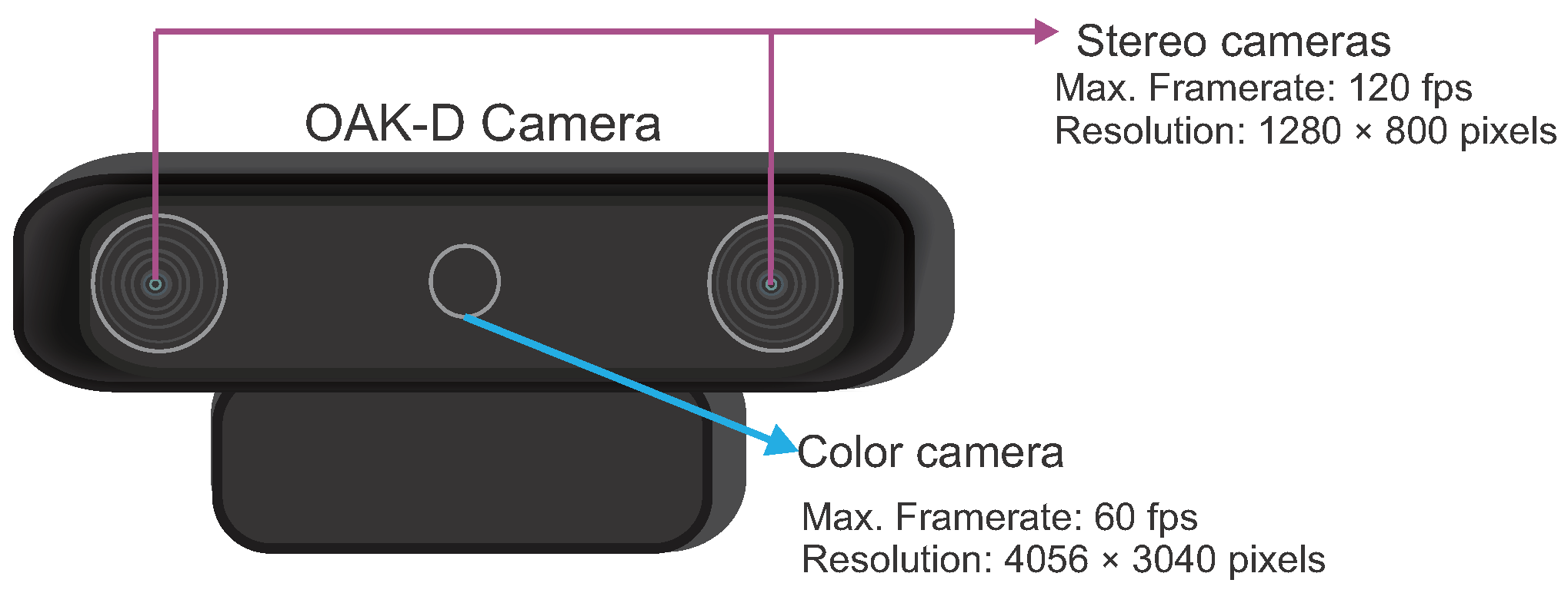
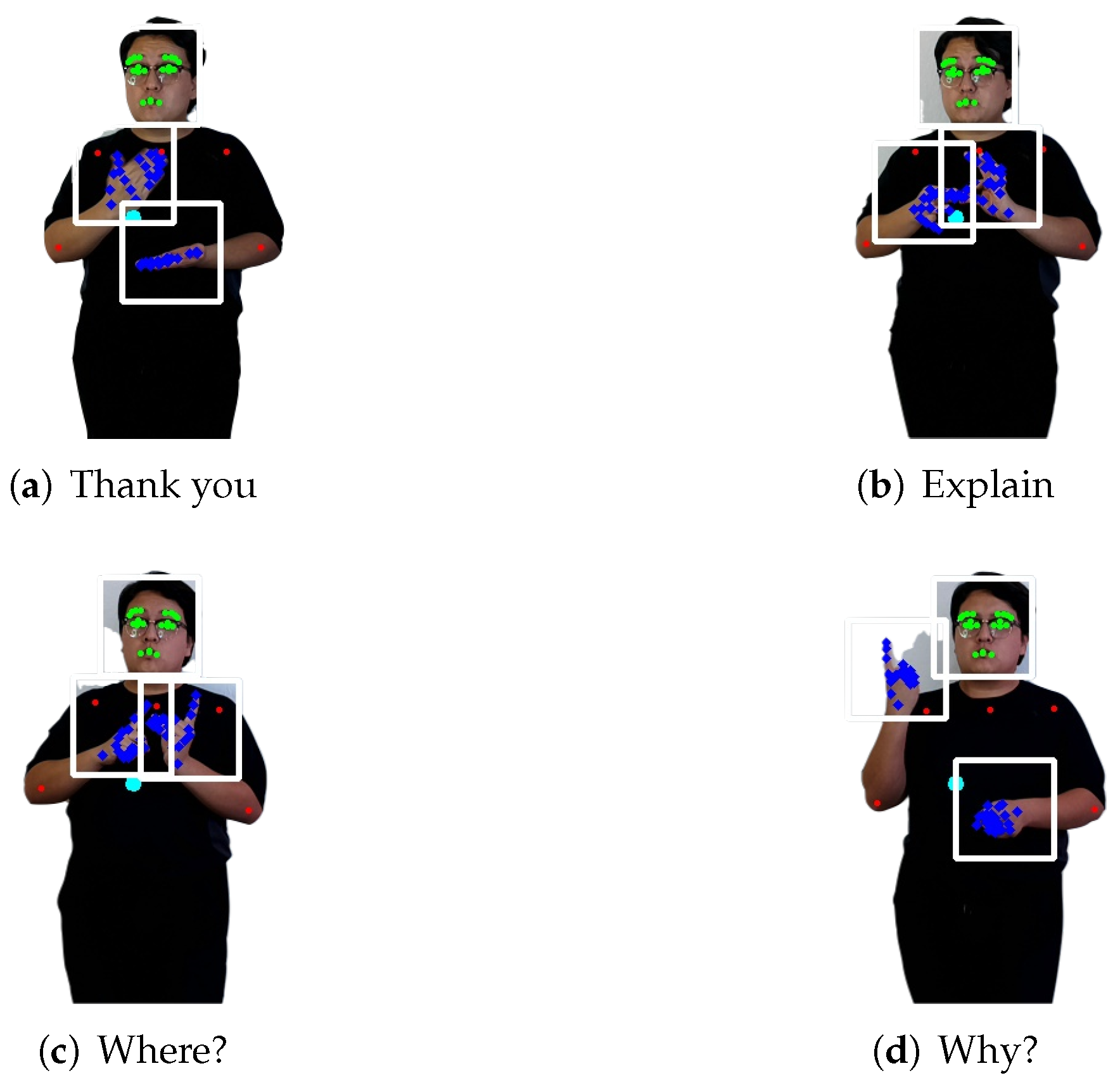
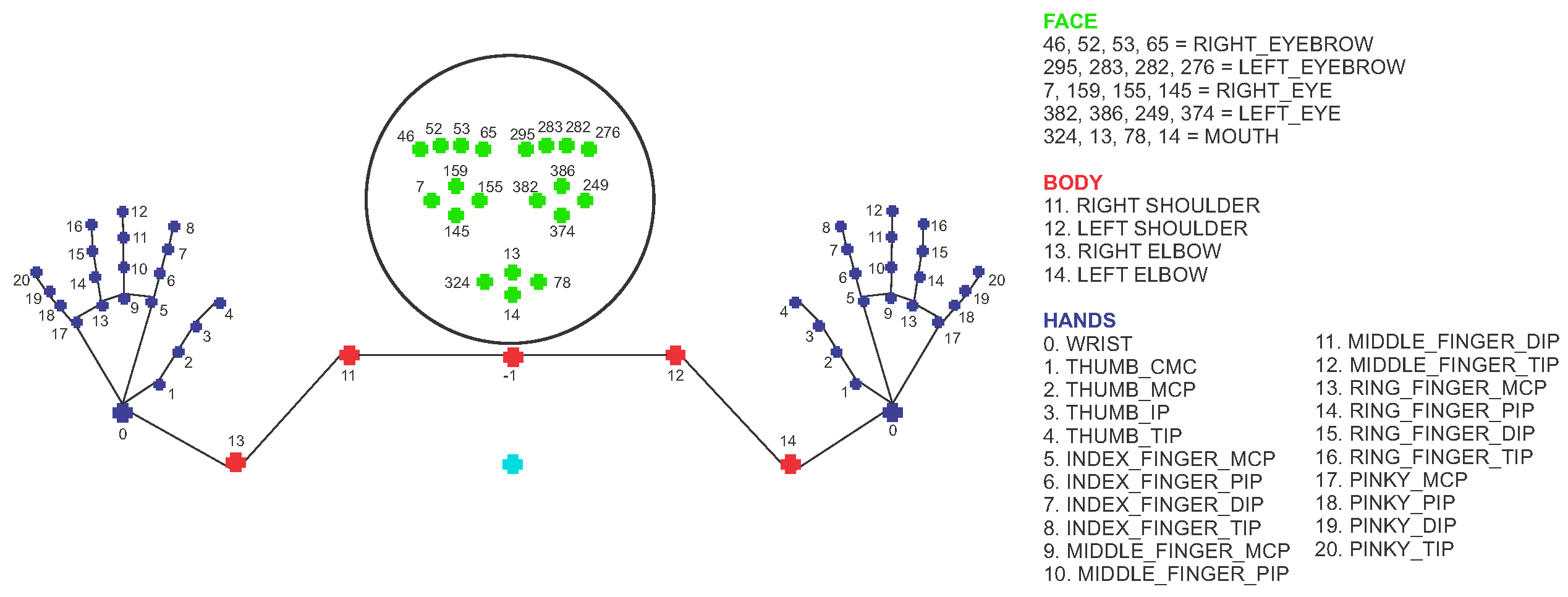
3.1. Data Acquisition

We collected a dataset of 30 different signs, each one performed 25 times by four different people at different speeds, starting and ending times. The full dataset consists of 3000 samples. Each sign is composed of 20 consecutive frames containing hands, body, and facial 3D keypoint coordinates.

We used an OAK-D camera for the data acquisition. This device consists of three cameras: a central camera to obtain RGB information and a stereo rig to get depth information from the disparity between images (see Figure 1).

We used the DepthAI [29] and the MediaPipe [30,31,32] libraries to detect the face, body, and hands keypoints. From the total set of 543 keypoints, we selected a subset 67 distributed as follows: 20 for the face, 5 for the body, and 21 for each hand, as shown in Figure 2.

The original facial keypoints include a dense face mesh containing 468 landmarks. Given that most of the face landmarks have a high correlation, we employ a feature selection approach to reduce the face landmarks down to 20, including four points for each eyebrow, four points around each eye, and four points around the mouth, as shown in Figure 2. Next, we selected the upper body points from the original body landmarks, including the chest, shoulders, and elbows. Since the MediaPipe library does not provide a chest point, we obtained it as the middle point between the shoulders. Finally, for the hands, we use all the landmarks that include four points on each finger and five points around each hand palm for a total of 21 points on each hand.

Figure 3 shows some examples of keypoints captured for the words: (a) thank you, (b) explain, (c) where? and (d) why? As part of the dataset, we stored the keypoints coordinated and the sequence of images for each sign.

We detect each keypoint in the RGB image and represent it by its $P^{\prime }[X^{\prime },Y^{\prime }]$ coordinates. For these coordinates we obtain its depth value Z from the depth image and compute the 3D space coordinates $P[X,Y,Z]$ using Equations (1) and (2).

$$\begin{array}{c}X=\left(\frac{X^{\prime }Z}{f}\right),\hfill \end{array}$$

(1)

$$\begin{array}{c}Y=\left(\frac{Y^{\prime }Z}{f}\right),\hfill \end{array}$$

(2)

where $X^{\prime }$ and $Y^{\prime }$ are the pixel coordinates in the image, f is the focal length, and Z the depth.

We collected samples for 30 different signs shown in

Table 2. Data corpus description.

Type of Sign	Sign	Static/Dynamic	One-Handed/Two-Handed	Symmetric/Asymmetric	Left Hand	Right Hand
Alphabet	A	Static	One-handed	Asymmetric	Without use	Dominant
	B	Static	One-handed	Asymmetric	Without use	Dominant
	C	Static	One-handed	Asymmetric	Without use	Dominant
	D	Static	One-handed	Asymmetric	Without use	Dominant
	J	Dynamic	One-handed	Asymmetric	Without use	Dominant
	K	Dynamic	One-handed	Asymmetric	Without use	Dominant
	Q	Dynamic	One-handed	Asymmetric	Without use	Dominant
	X	Dynamic	One-handed	Asymmetric	Without use	Dominant
Questions	What?	Dynamic	Two-handed	Symmetric	Simultaneous	Simultaneous
	When?	Dynamic	One-handed	Asymmetric	Without use	Dominant
	How much?	Dynamic	Two-handed	Symmetric	Simultaneous	Simultaneous
	Where?	Dynamic	Two-handed	Asymmetric	Base	Dominant
	For what?	Dynamic	One-handed	Asymmetric	Without use	Dominant
	Why?	Dynamic	One-handed	Asymmetric	Base	Dominant
	What is that?	Dynamic	One-handed	Asymmetric	Without use	Dominant
	Who?	Dynamic	Two-handed	Asymmetric	Base	Dominant
Days of the week	Monday	Dynamic	One-handed	Asymmetric	Without use	Dominant
	Tuesday	Dynamic	One-handed	Asymmetric	Without use	Dominant
	Wednesday	Dynamic	One-handed	Asymmetric	Without use	Dominant
	Thursday	Dynamic	One-handed	Asymmetric	Without use	Dominant
	Friday	Dynamic	One-handed	Asymmetric	Without use	Dominant
	Saturday	Dynamic	One-handed	Asymmetric	Without use	Dominant
	Sunday	Dynamic	One-handed	Asymmetric	Without use	Dominant
Frequent words	Spell	Dynamic	One-handed	Asymmetric	Without use	Dominant
	Explain	Dynamic	Two-handed	Asymmetric	Alternate	Alternate
	Thank you	Dynamic	Two-handed	Asymmetric	Base	Dominant
	Name	Dynamic	One-handed	Asymmetric	Without use	Dominant
	Please	Dynamic	Two-handed	Symmetric	Simultaneous	Simultaneous
	Yes	Dynamic	One-handed	Asymmetric	Without use	Dominant
	No	Dynamic	One-handed	Asymmetric	Without use	Dominant

. Out of these, four are static, and 26 are dynamic. In terms of the hands used, 17 are one-handed and 13 two-handed. They can also be classified into four subgroups: 8 are letters of the sign-language alphabet, 8 are questions, 7 are days of the week, and 7 are common phrases.

The captured data is stored in comma-separated values (CSV) structured in 20 rows and 201 columns. Each file represents a single repetition of an individual sign, and each row represents the information obtained in a single image.

Each row contains the keypoints (X, Y, Z) coordinates in the following order: five body keypoints, 20 facial keypoints, 21 left-hand keypoints, and 21 right-hand keypoints. The coordinates are in meters and normalized with respect to the chest to make the signs invariant to camera distance.

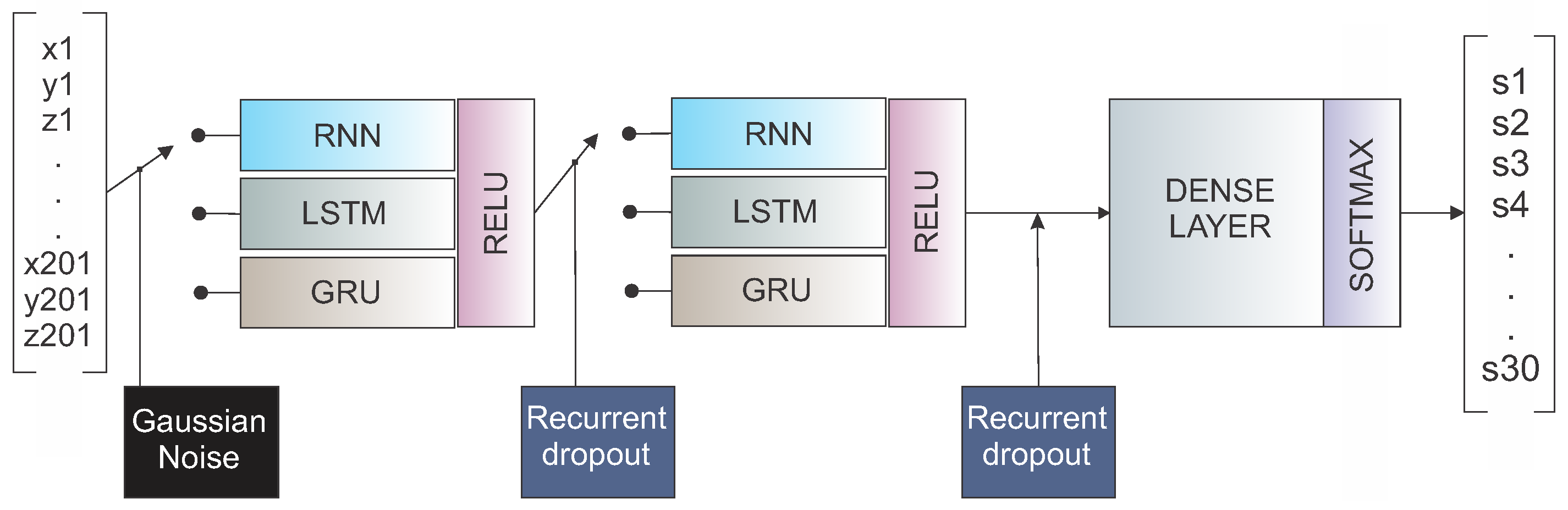
3.2. Classification Architectures

For classification, we evaluated three different architectures: recurrent neural network (RNN), long short-term memory (LSTM), and gated recurrent unit (GRU). We selected these architectures due to the data characteristics, consisting of temporal sequences. As indicated in the work of Sak et al. [33] unlike feedforward networks, RNNs have cyclic connections that make them powerful for modeling sequences. However, it is well known that this model has problems updating weights, resulting in gradient vanishing and gradient exploding errors. If the weight is too small, the gradient will disappear, i.e., it will not continue learning, and in the opposite case, if large gradients accumulate, they will result in large weight updates causing the gradient to explode [34]. The LSTM and GRU variations of the RNN were developed to address the problems above.

Figure 4 shows the model architectures used in this work. The input is conformed by a vector containing the hands, body, and face keypoints’ x, y, and z coordinates. We either used an RNN, an LSTM, or a GRU with recurrent dropout and ending with a dense layer.

In the following, we describe these three architectures.

3.2.1. Recurrent Neural Network (RNN)

A recurrent neural network or RNN, is a model that starts from the same premises as a regular artificial neural network (ANN), but adds a recurrence of the output values to the neuron’s input. With this, the neurons receive the output value of the previous neurons, influencing the network’s behavior to take into account past data.

3.2.2. Long Short-Term Memory (LSTM)

A long short-term memory, or LSTM, is a type of recurrent neural network model proposed by Hochreiter and Schmidhuber in 1997 [35] capable of learning longer sequences of data by reducing the gradient vanishing problem. The LSTM architecture consists of recursively connected subnetworks known as memory cell blocks. Each block contains self-connected memory cells and multiplicative units that learn to open and close access to the constant error stream, allowing LSTM memory cells to store and access information for long periods. In addition, there are forget gates within an LSTM network, which provide continuous instructions for writing, reading, and reset operations for the cells.

3.2.3. GRU

The GRU is a more recent recurrent network initially created for machine translation tasks. This model is similar to the LSTM because it can capture long-term dependencies. However, unlike the LSTM, this model does not require internal memory cells, reducing complexity. A GRU unit combines the forgetting gate and the input gate into a single update gate; it also integrates the cell state and the hidden state, solving local minima stalling and gradient descent problems. A main advantage of the GRU over the LSTM is that it requires less computational resources by having a less complex structure.

3.3. Classification

We split the dataset into three parts, 70% for training data, 15% for validation, and 15% for testing. We trained all models for 300 epochs using early stopping with a patience of 100 epochs using the categorical cross-entropy loss function and Adam optimizer. We used Keras [36] and Tensorflow libraries [37].

Table 3. Model variations used for classification.

Network	Layer 1 Units	Layer 2 Units	Parameters (Thousands)
RNN	32	16	8.782
	64	32	21.118
	128	64	56.542
	256	128	170.398
	512	256	570.142
	1024	512	2057.758
LSTM	32	16	33.60
	64	32	81.502
	128	64	220.318
	256	128	669.982
	512	256	2257.438
	1024	512	8184.862
GRU	32	16	25.47
	64	32	61.662
	128	64	166.302
	256	128	504.606
	512	256	1697.31
	1024	512	6147.102

shows the different model architectures that we used in this work.

For training, we optionally added online augmentation of Gaussian noise to the input keypoints with a mean of zero and standard deviation of 30 cm. This produces the effect of randomly varying the keypoints from the detected position simulating different ways to perform a sign. The noise is added at every input during training, generating different values on every iteration. This approach also helps to reduce overfitting and improve generalization.

Figure 5 shows the validation accuracy during training for the models with 32 units on the first layer and 16 units on the second layer.

3.4. Evaluation

To evaluate the performance of our method, we calculate the precision, recall, and accuracy. These metrics are based on the correctly/incorrectly classified signs which are defined with the true positives ($TP$), false positives ($FP$), true negatives ($TN$), and false negatives ($FN$) described below [38]:

• True Positive ($TP$) refers to the number of predictions where the classifier correctly predicts the positive class as positive.
• True Negative ($TN$) indicates to the number of predictions where the classifier correctly predicts the negative class as negative.
• False Positive ($FP$) denotes to the number of predictions where the classifier incorrectly predicts the negative class as positive.
• False Negative ($FN$) refers to the number of predictions where the classifier incorrectly predicts the positive class as negative.

The precision indicates the proportion of positive identifications that were actually correct. The precision is calculated with Equation (3).

$$Precision=\frac{TP}{TP+FP}$$

(3)

The recall represents the proportion of actual positives correctly identified. The recall is calculated with Equation (4).

$$Recall=\frac{TP}{TP+FN}$$

(4)

The accuracy measures how often the predictions match the labels, that is, the percentage of predicted values that correspond with actual values with Equation (5).

$$Accuracy=\frac{TP+TN}{TP+TN+FP+FN}$$

(5)

The next section describe the results obtained.

4. Results

After training the models listed in Table 3, we obtained the results shown in

Table 4. Testing accuracy for the different model architectures. The bold numbers represent the variation (row) with the best accuracy. Model variations with large number of units overfit the training data performing poorly on the test data.

Network	Layer 1 Units	Layer 2 Units	Accuracy (Percentage)
RNN	32	16	93.11
	64	32	94.22
	128	64	94.0
	256	128	92.44
	512	256	61.55
	1024	512	57.55
LSTM	32	16	92.44
	64	32	96.44
	128	64	96.22
	256	128	96.44
	512	256	96.66
	1024	512	95.77
GRU	32	16	96.22
	64	32	96.44
	128	64	96.44
	256	128	96.66
	512	256	97.11
	1024	512	95.77

. From these results, we found that all architectures overfit with larger model sizes. Additionally, the RNN tends to overfit with less number of units than LSTM and GRU, and GRU delivered the best accuracy at 97.11% for the model comprising 512 units on the first layer and 256 units on the second layer.

Figure 6 shows the precision and recall curves for the best model variation of each architecture shown in Table 4. GRU performed slightly better than LSTM with less model complexity as shown in Table 3.

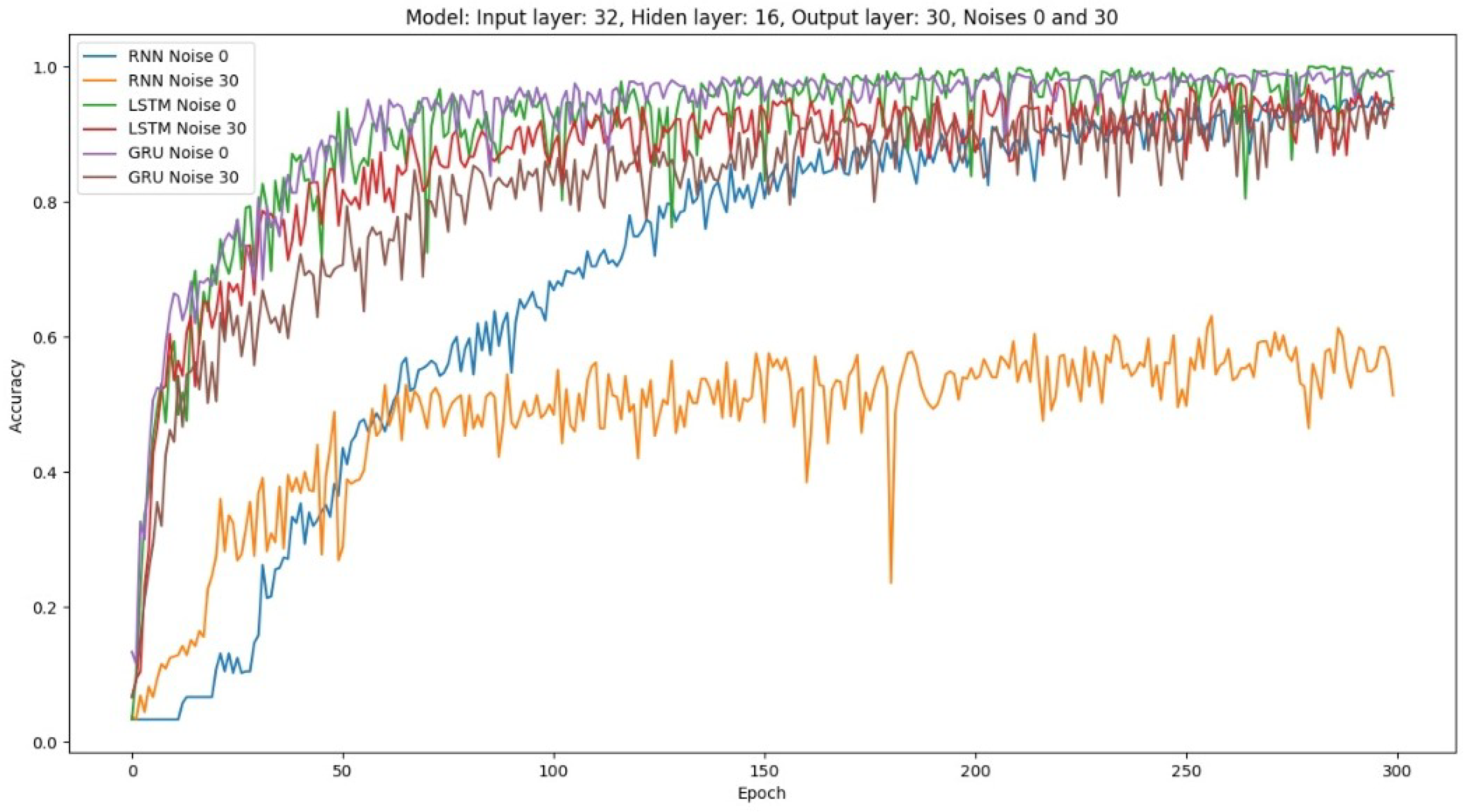
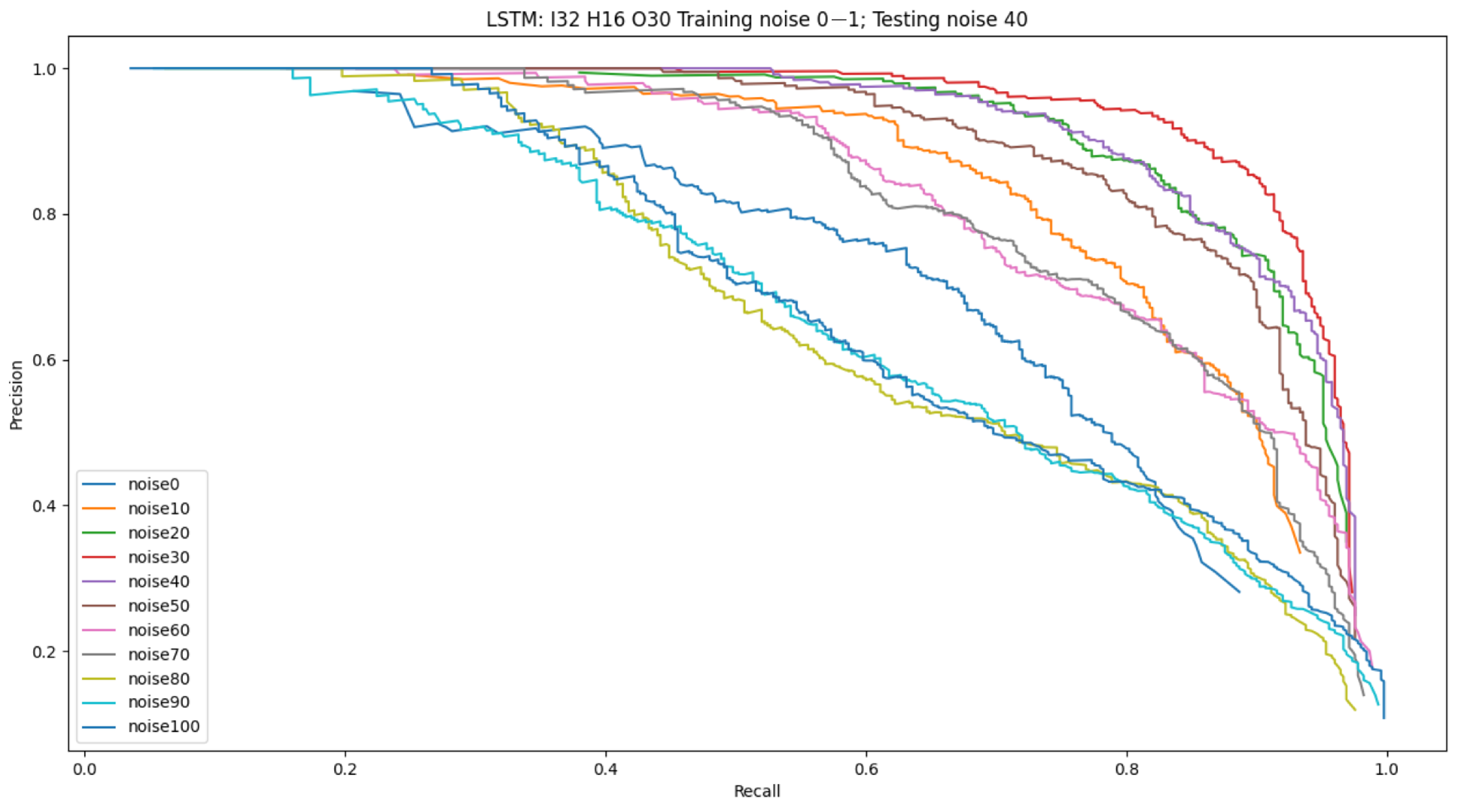
4.1. System Robustness to Noise

To evaluate the system’s robustness to noise, we created five additional testing sets with different levels of Gaussian noise in the keypoints coordinates. The noise levels went from zero to 50 cm of standard deviation in increasing steps of 10 cm.

Table 5. Classification accuracy of the best model variation of each architecture evaluated on noisy testing data. The names ending with aug refer to a model augmented during training with Gaussian noise on the inputs of zero mean and standard deviation of 30 cm. Every column represents a test set with a different noise level. The best result on each column is highlighted in bold.

Best Model	Testing Noise
	No-Noise	10 cm	20 cm	30 cm	40 cm	50 cm
RNN	92.44	45.11	45.33	46.44	46.44	46.88
RNN aug	63.55	60.44	58.44	60.0	59.33	59.33
LSTM	96.66	66.22	65.33	63.11	67.77	62.44
LSTM aug	95.55	89.33	90.44	89.11	90.44	88.88
GRU	97.11	48.22	50.66	51.11	46.44	46.66
GRU aug	96.22	69.11	69.33	68.66	68.44	67.33

shows the testing accuracies of the best model variation from each architecture evaluated on different testing sets. The models ending with aug are the ones augmented during training with Gaussian noise on the inputs as described in Section 3.3.

From the results of Table 5 we can conclude that the LSTM model is more robust to noise than the RNN and GRU models. Additionally, adding Gaussian noise during training helped significantly. Due to this, we selected a small LSTM architecture with 32 units on the first layer and 16 units on the second layer and trained multiple models with increasing levels of Gaussian noise augmentation to the inputs going from 0 to 100 cm of standard deviation.

Table 6. Classification accuracy of multiple LSTM models trained with different levels of noise augmentation to the inputs evaluated on noisy testing sets. The best result on each column is highlighted in bold.

LSTM Model	Testing Noise
	No-Noise	10 cm	20 cm	30 cm	40 cm	50 cm
0 cm	92.44	66.22	65.33	63.11	67.77	62.66
10 cm	96.44	74.22	74.66	74.44	75.33	72.66
20 cm	94.88	84.22	82.44	79.55	83.11	84.22
30 cm	93.11	86.0	87.33	85.11	87.11	87.11
40 cm	81.55	80.66	81.77	79.55	83.33	82.88
50 cm	82.44	79.77	78.22	79.55	80.66	79.77
60 cm	68.44	68.88	71.77	70.0	71.33	72.44
70 cm	70.66	71.55	71.33	70.0	72.88	69.55
80 cm	59.33	58.22	56.44	57.11	57.55	59.33
90 cm	61.11	57.77	58.22	59.55	58.22	60.22
100 cm	61.33	58.66	60.22	57.55	58.44	60.22

shows the accuracy of these LSTM models evaluated on multiple testing noise levels. This table indicates that a Gaussian noise augmentation of 30 cm of standard deviation gave the best results for increasing noise levels on the test data.

Figure 7 shows the precision and recall curves for these different models evaluated on the testing set with Gaussian noise of 40 cm of standard deviation. The figure demonstrates that the best model corresponds to the one trained with Gaussian noise of 30 cm of standard deviation.

In the next section, we report the results of a set of ablation studies aimed to study the performance of our classifier at different model depths and a different set of input features to understand the contribution to the overall system.

4.2. Ablation Studies

We performed two ablations studies. In the first one, we varied the architecture of the LSTM model by removing and adding layers and dropout units. In the second experiment, we removed input features to determine how each keypoint set contributes to the prediction.

4.2.1. Varying Architecture

In this experiment, we evaluated the performance of different architectures. We trained models using one, two, and three layers and using noise augmentation and dropout.

Table 7. Varying architecture results. Each row represents a trained model with either one, two or three layer; as well as with and without noise augmentation and recurrent dropout. The best result on each column is highlighted in bold.

Number of Layers	Noise Aug	Dropout	Testing Noise
			No-Noise	10 cm	20 cm	30 cm	40 cm	50 cm
One layer	No	No	96.44	58.44	60.66	60.0	56.44	56.22
One layer	No	Yes	96.44	58.44	57.77	52.22	56.88	56.88
One layer	Yes	No	88.22	82.22	81.55	80.88	83.11	82.0
One layer	Yes	Yes	94.88	88.22	87.77	89.33	87.55	88.44
Two layers	No	No	96.22	34.22	36.22	38.0	35.33	37.11
Two layers	No	Yes	96.44	39.11	39.33	36.22	37.55	37.11
Two layers	Yes	No	94.44	87.11	87.77	88.66	88.44	88.66
Two layers	Yes	Yes	95.55	89.33	90.44	88.44	89.33	88.44
Three layers	No	No	92.0	27.33	30.0	28.88	28.66	24.88
Three layers	No	Yes	97.33	38.0	34.88	34.44	35.77	34.88
Three layers	Yes	No	94.0	88.66	86.88	84.22	86.22	86.44
Three layers	Yes	Yes	96.66	88.0	88.88	88.88	89.11	89.11

shows that in most cases, the two-layer model performed better than the others. The results also demonstrate that the noise augmentation plus the recurrent dropout units help in all cases with testing noise, but do not help with non-noise testing.

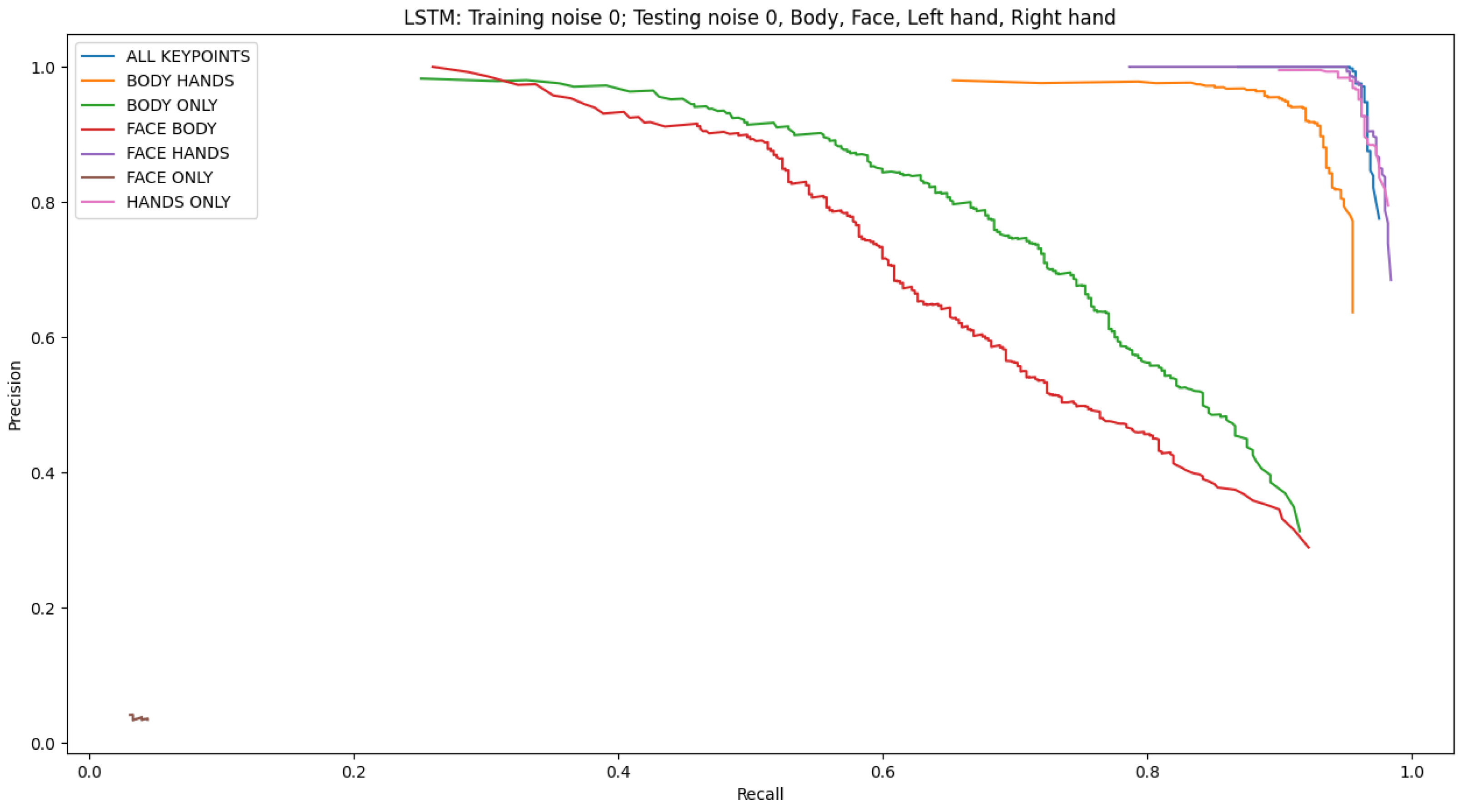
4.2.2. Varying Features

We tried different combinations of body keypoints and input features in this experiment. For example, using hands-only, body-only, face-only, and their combinations.

Table 8. Model accuracy when varying the input features. Every row reports the results of a model training with a specific set of features. For example, the row names All features used hands, body, and face keypoints. The best result on each column is highlighted in bold.

Features Combination	Testing Noise
	No-Noise	10 cm	20 cm	30 cm	40 cm	50 cm
All features	96.44	64.44	63.55	61.77	63.55	62.44
Hands-only	96.0	69.11	69.33	68.66	68.44	66.0
Face-only	3.55	5.11	5.55	4.22	5.77	4.0
Body-only	71.55	8.66	10.44	10.22	10.66	10.0
Face + Body	63.55	12.88	12.44	12.88	10.88	13.77
Hands + Face	96.22	56.88	58.44	58.0	58.22	58.88
Hands + Body	92.0	65.55	68.22	65.33	66.22	67.33

shows the results. The table denotes that using all the features delivered the best results when the testing data is not noisy. When adding noise to the testing, the hands-only features performed the best. This phenomenon can be explained because the keypoints on the face are very close to each other, such that the added noise changes the face structure completely.

Figure 8 shows the precision/recall curves for the models with different combinations of input features evaluated on the testing data without added noise. The curves reveal that all the sets containing the hands obtained similar results, as shown in the upper right of the graph. On the contrary, features set not having the hands perform worse. This suggests that hands are the most important features for sign language recognition. As expected, face-only keypoints obtained the worst results, as depicted by the small curve in the lower left.

5. Discussion

After comparing the three most common architectures for sequence classification, we found that the architecture based on LSTM performed the best when the inputs were noisy. On the other hand, GRU performed better when the inputs were not noisy. We also demonstrate that training with Gaussian noise augmentation to the inputs makes the system more robust and can generalize better.

One ablation study demonstrated that a more extensive network was not better, and the optimal size was a 2-layer network with noise augmentation and dropout.

The second ablation study showed that the hands’ keypoints are the most important features for classification with a 96% accuracy, followed by body features with 72% accuracy. Facial keypoints alone are not good features, with an accuracy of 4%; however, when combined with the hand keypoints, the accuracy increased to 96.2%. The best model was the one mixing the three sets of keypoints with an accuracy of 96.44%, proving our hypothesis that the facial and body features play a role on the sign language recognition. This second ablation study also showed that adding Gaussian noise to the facial keypoints affects model accuracy. The hands-only model had an accuracy of 69%, and a model using hands plus face had a lower accuracy of 57%.

6. Conclusions

In this paper, we developed a method for sign language recognition using a RGB-D camera. We detect the hands, body, and facial features, convert them to 3D and use them as input features for classifiers based on recurrent neural networks. We compare three different architectures: recurrent neural networks (RNN), long short-term memories (LSTM), and gated recurrent units (GRU). LSTM performed the best with noisy inputs, and GRU performed best without noisy inputs and less trainable parameters.

We collected a dataset of 30 dynamic signs from the Mexican Sign Language with 100 samples of each sign and used it for training, validation, and testing. Our best model obtained an accuracy above 97% on the test set.

We want to extend the number of signs to recognize and integrate this method in a prototype in future work.

References

1. INEGI. Las Personas Con Discapacidad Auditiva. Available online: https://www.inegi.org.mx/app/tabulados/interactivos/?pxq=Discapacidad_Discapacidad_02_2c111b6a-6152-40ce-bd39-6fab2c4908e3&idrt=151&opc=t (accessed on 5 May 2021).
2. Serafín, M.; González, R. Manos Con Voz, Diccionario de Lenguaje de señas Mexicana, 1st ed.; Committee on the Elimination of Racial Discrimination: Mexico City, Mexico, 2011; pp. 15–19. [Google Scholar]
3. Torres, S.; Sánchez, J.; Carratalá, P. Curso de Bimodal. In Sistemas Aumentativos de Comunicación; Universidad de Málaga: Málaga, Spain, 2008. [Google Scholar]
4. WFD-SNAD. Informe de la Encuesta Global de la Secretaría Regional de la WFD para México, América Central y el Caribe (WFD MCAC) Realizado por la Federación Mundial de Sordos y la Asociación Nacional de Sordos de Suecia. 2008, p. 16. Available online: https://docplayer.es/12868567-Este-proyecto-se-realizo-bajo-los-auspicios-de-la-asociacion-nacional-de-sordos-de-suecia-sdr-y-la-federacion-mundial-de-sordos-wfd-con-la.html (accessed on 12 March 2021).
5. Ruvalcaba, D.; Ruvalcaba, M.; Orozco, J.; López, R.; Cañedo, C. Prototipo de guantes traductores de la lengua de señas mexicana para personas con discapacidad auditiva y del habla. In Proceedings of the Congreso Nacional de Ingeniería Biomédica, Leon Guanajuato, Mexico, 18–20 October 2018; SOMIB Volume 5, pp. 350–353. [Google Scholar]
6. Saldaña González, G.; Cerezo Sánchez, J.; Bustillo Díaz, M.M.; Ata Pérez, A. Recognition and classification of sign language for spanish. Comput. Sist. 2018, 22, 271–277. [Google Scholar] [CrossRef]
7. Varela-Santos, H.; Morales-Jiménez, A.; Córdova-Esparza, D.M.; Terven, J.; Mirelez-Delgado, F.D.; Orenday-Delgado, A. Assistive Device for the Translation from Mexican Sign Language to Verbal Language. Comput. Sist. 2021, 25, 451–464. [Google Scholar] [CrossRef]
8. Cuecuecha-Hernández, E.; Martínez-Orozco, J.J.; Méndez-Lozada, D.; Zambrano-Saucedo, A.; Barreto-Flores, A.; Bautista-López, V.E.; Ayala-Raggi, S.E. Sistema de reconocimiento de vocales de la Lengua de Señas Mexicana. Pist. Educ. 2018, 39, 128. [Google Scholar]
9. Estrivero-Chavez, C.; Contreras-Teran, M.; Miranda-Hernandez, J.; Cardenas-Cornejo, J.; Ibarra-Manzano, M.; Almanza-Ojeda, D. Toward a Mexican Sign Language System using Human Computer Interface. In Proceedings of the 2019 International Conference on Mechatronics, Electronics and Automotive Engineering (ICMEAE), Cuernavaca, Mexico, 26–29 November 2019; pp. 13–17. [Google Scholar]
10. Solís, F.; Toxqui, C.; Martínez, D. Mexican sign language recognition using jacobi-fourier moments. Engineering 2015, 7, 700. [Google Scholar] [CrossRef] [Green Version]
11. Cervantes, J.; García-Lamont, F.; Rodríguez-Mazahua, L.; Rendon, A.Y.; Chau, A.L. Recognition of Mexican sign language from frames in video sequences. In International Conference on Intelligent Computing; Springer: Lanzhou, China, 2016; pp. 353–362. [Google Scholar]
12. Martínez-Gutiérrez, M.; Rojano-Cáceres, J.R.; Bárcenas-Patiño, I.E.; Juárez-Pérez, F. Identificación de lengua de señas mediante técnicas de procesamiento de imágenes. Res. Comput. Sci. 2016, 128, 121–129. [Google Scholar] [CrossRef]
13. Solís, F.; Martínez, D.; Espinoza, O. Automatic mexican sign language recognition using normalized moments and artificial neural networks. Engineering 2016, 8, 733–740. [Google Scholar] [CrossRef] [Green Version]
14. Pérez, L.M.; Rosales, A.J.; Gallegos, F.J.; Barba, A.V. LSM static signs recognition using image processing. In Proceedings of the 2017 14th International Conference on Electrical Engineering, Computing Science and Automatic Control (CCE), Mexico City, Mexico, 20–22 October 2017; pp. 1–5. [Google Scholar]
15. Mancilla-Morales, E.; Vázquez-Aparicio, O.; Arguijo, P.; Meléndez-Armenta, R.Á.; Vázquez-López, A.H. Traducción del lenguaje de senas usando visión por computadora. Res. Comput. Sci. 2019, 148, 79–89. [Google Scholar] [CrossRef]
16. Martinez-Seis, B.; Pichardo-Lagunas, O.; Rodriguez-Aguilar, E.; Saucedo-Diaz, E.R. Identification of Static and Dynamic Signs of the Mexican Sign Language Alphabet for Smartphones using Deep Learning and Image Processing. Res. Comput. Sci. 2019, 148, 199–211. [Google Scholar] [CrossRef]
17. Galicia, R.; Carranza, O.; Jiménez, E.; Rivera, G. Mexican sign language recognition using movement sensor. In Proceedings of the 2015 IEEE 24th International Symposium on Industrial Electronics (ISIE), Buzios, Brazil, 3–5 June 2015; pp. 573–578. [Google Scholar]
18. Sosa-Jiménez, C.O.; Ríos-Figueroa, H.V.; Rechy-Ramírez, E.J.; Marin-Hernandez, A.; González-Cosío, A.L.S. Real-time mexican sign language recognition. In Proceedings of the 2017 IEEE International Autumn Meeting on Power, Electronics and Computing (ROPEC), Ixtapa, Mexico, 8–10 November 2017; pp. 1–6. [Google Scholar]
19. García-Bautista, G.; Trujillo-Romero, F.; Caballero-Morales, S.O. Mexican sign language recognition using kinect and data time warping algorithm. In Proceedings of the 2017 International Conference on Electronics, Communications and Computers (CONIELECOMP), Cholula, Mexico, 22–24 February 2017; pp. 1–5. [Google Scholar]
20. Jimenez, J.; Martin, A.; Uc, V.; Espinosa, A. Mexican sign language alphanumerical gestures recognition using 3D Haar-like features. IEEE Lat. Am. Trans. 2017, 15, 2000–2005. [Google Scholar] [CrossRef]
21. Martínez-Gutiérrez, M.E.; Rojano-Cáceres, J.R.; Benítez-Guerrero, E.; Sánchez-Barrera, H.E. Data Acquisition Software for Sign Language Recognition. Res. Comput. Sci. 2019, 148, 205–211. [Google Scholar] [CrossRef]
22. Unutmaz, B.; Karaca, A.C.; Güllü, M.K. Turkish sign language recognition using kinect skeleton and convolutional neural network. In Proceedings of the 2019 27th Signal Processing and Communications Applications Conference (SIU), Sivas, Turkey, 24–26 April 2019; pp. 1–4. [Google Scholar]
23. Jing, L.; Vahdani, E.; Huenerfauth, M.; Tian, Y. Recognizing american sign language manual signs from rgb-d videos. arXiv 2019, arXiv:1906.02851. [Google Scholar]
24. Raghuveera, T.; Deepthi, R.; Mangalashri, R.; Akshaya, R. A depth-based Indian sign language recognition using microsoft kinect. Sādhanā 2020, 45, 1–13. [Google Scholar] [CrossRef]
25. Khan, M.; Siddiqui, N. Sign Language Translation in Urdu/Hindi Through Microsoft Kinect. In IOP Conference Series: Materials Science and Engineering; IOP Publishing: Topi, Pakistan, 2020; Volume 899, p. 012016. [Google Scholar]
26. Xiao, Q.; Qin, M.; Yin, Y. Skeleton-based Chinese sign language recognition and generation for bidirectional communication between deaf and hearing people. Neural Netw. 2020, 125, 41–55. [Google Scholar] [CrossRef] [PubMed]
27. Trujillo-Romero, F.; Bautista, G.G. Reconocimiento de palabras de la Lengua de Señas Mexicana utilizando información RGB-D. ReCIBE Rev. Electron. Comput. Inform. Biomed. Electron. 2021, 10, C2–C23. [Google Scholar]
28. Carmona-Arroyo, G.; Rios-Figueroa, H.V.; Avendaño-Garrido, M.L. Mexican Sign-Language Static-Alphabet Recognition Using 3D Affine Invariants. In Machine Vision Inspection Systems: Machine Learning-Based Approaches; Scrivener Publishing LLC: Beverly, MA, USA, 2021; Volume 2, pp. 171–192. [Google Scholar]
29. DepthAI. DepthAI’s Documentation. Available online: https://docs.luxonis.com/en/latest/ (accessed on 31 March 2021).
30. MediaPipe. MediaPipe Holistic. Available online: https://google.github.io/mediapipe/solutions/holistic#python-solution-api (accessed on 29 March 2021).
31. Zhang, F.; Bazarevsky, V.; Vakunov, A.; Tkachenka, A.; Sung, G.; Chang, C.L.; Grundmann, M. Mediapipe hands: On-device real-time hand tracking. arXiv 2020, arXiv:2006.10214. [Google Scholar]
32. Singh, A.K.; Kumbhare, V.A.; Arthi, K. Real-Time Human Pose Detection and Recognition Using MediaPipe. In International Conference on Soft Computing and Signal Processing; Springer: Hyderabad, India, 2021; pp. 145–154. [Google Scholar]
33. Sak, H.; Senior, A.; Beaufays, F. Long short-term memory based recurrent neural network architectures for large vocabulary speech recognition. arXiv 2014, arXiv:1402.1128. [Google Scholar]
34. Yang, S.; Yu, X.; Zhou, Y. Lstm and gru neural network performance comparison study: Taking yelp review dataset as an example. In Proceedings of the 2020 International Workshop on Electronic Communication and Artificial Intelligence (IWECAI), Qingdao, China, 12–14 June 2020; pp. 98–101. [Google Scholar]
35. Hochreiter, S.; Schmidhuber, J. Long short-term memory. Neural Comput. 1997, 9, 1735–1780. [Google Scholar] [CrossRef] [PubMed]
36. Chollet, F. Deep Learning with Python, 1st ed.; Manning Publications Co.: Shelter Island, NY, USA, 2018; pp. 178–232. [Google Scholar]
37. Abadi, M.; Agarwal, A.; Barham, P.; Brevdo, E.; Chen, Z.; Citro, C.; Corrado, G.S.; Davis, A.; Dean, J.; Devin, M.; et al. TensorFlow: Large-scale machine learning on heterogeneous systems. arXiv 2016, arXiv:1603.04467. [Google Scholar]
38. Kuhn, M.; Johnson, K. Applied Predictive Modeling; Springer: New York, NY, USA, 2013; Volume 26. [Google Scholar]
Figure 1. OAK-D Camera.
Applsci 12 05523 g001
Figure 2. Face, body, and hand selected keypoints. The numbers indicate the landmark indices used in the MediaPiple library.
Applsci 12 05523 g002
Figure 3. Facial, hands, and body keypoints for the signs representing the words: (a) Thank you, (b) Explain, (c) Where? and (d) Why?
Applsci 12 05523 g003
Figure 4. Recurrent neural network architectures.
Applsci 12 05523 g004
Figure 5. Training curves for the models with 32 neurons. Best seen in color.
Applsci 12 05523 g005
Figure 6. Precision recall curves for the best model of each architecture.
Applsci 12 05523 g006
Figure 7. Precision and recall curves for the models presented in Table 6 evaluated on a testing set with Gaussian noise of zero mean and 40 cm of standard deviation.
Applsci 12 05523 g007
Figure 8. Precision recall curves for features combinations.
Applsci 12 05523 g008