Article

Statistical Data-Driven Model for Hardness Prediction in Austempered Ductile Irons

by
Nelly Abigaíl Rodríguez-Rosales
1,
Félix Alan Montes-González
1,
Oziel Gómez-Casas
2,
Josué Gómez-Casas
2,
Jesús Salvador Galindo-Valdés
2,
Juan Carlos Ortiz-Cuellar
2,
Jesús Fernando Martínez-Villafañe
2,
Daniel García-Navarro
1 and
Carlos Rodrigo Muñiz-Valdez
2,*
1
Departamento de Metal Mecánica, Tecnológico Nacional de México/I.T. Saltillo, Saltillo 25280, Coahuila, Mexico
2
Facultad de Ingeniería, Universidad Autónoma de Coahuila, Arteaga 25350, Coahuila, Mexico
*
Author to whom correspondence should be addressed.
Metals 2022, 12(4), 676; https://doi.org/10.3390/met12040676
Submission received: 3 March 2022 / Revised: 6 April 2022 / Accepted: 9 April 2022 / Published: 15 April 2022

Abstract

:
This research evaluates the effect of temperature and time austempering on microstructural characteristics and hardness of ductile iron, validating the results by means of a statistical method for hardness prediction. Ductile iron was subjected to austenitization at 950 °C for 120 min and then to austempering heat treatment in a salt bath at temperatures of 290, 320, 350 and 380 °C for 30, 60, 90 and 120 min. By increasing austempering temperature, a higher content of carbon-rich austenite was obtained, and the morphology of the thin acicular ferrite needles produced at 290 °C turned completely feathery at 350 and 380 °C. A thickening of acicular ferrite needles was also observed as austempering time increased. An inversely proportional behavior of hardness values was thus obtained, which was validated through data analysis, statistical tools and a regression model taking temperature and time austempering as input variables and hardness as the output variable, which achieved a correlation among variables of about 97%. The proposal of a mathematical model for the prediction of hardness in austempered ductile iron represents a numerical approximation which validates the experimental results at 95.20%.

1. Introduction

Austempered ductile irons (ADIs) are noticeable materials in the industrial market since the spheroidal shape of graphite provides high fatigue resistance compared to other graphitic morphologies, such as lamellar in gray cast iron, offering better continuity of the iron metal matrix [1]. Likewise, austempering heat treatment affords an excellent combination of properties, e.g., high toughness, good ductility and high wear resistance [2,3]. The successful production of high-performance components from ADI requires a solid understanding of microstructural changes caused by alterations in processing parameters, such as austempering heat treatment variables and chemical composition, as they considerably modify mechanical properties.
Currently, the industrial sector aims to satisfy economic and ecological initiatives of cost and environmental footprint reduction in manufacturing processes by creating materials with excellent mechanical properties and low density and proposing new materials to replace those commonly used [3]. ADIs are attractive as substitutes for steel and aluminum components due to low manufacturing costs and lower environmental impact as well as mechanical properties comparable to steel and superior to aluminum [3,4,5,6,7,8].
The outstanding mechanical properties of ADI derive from the unique ausferritic microstructure composed of graphite nodules (G), carbon-rich austenite (γhC) and acicular ferrite (αac). These phases are yielded through the application of a thermal cycle comprising:
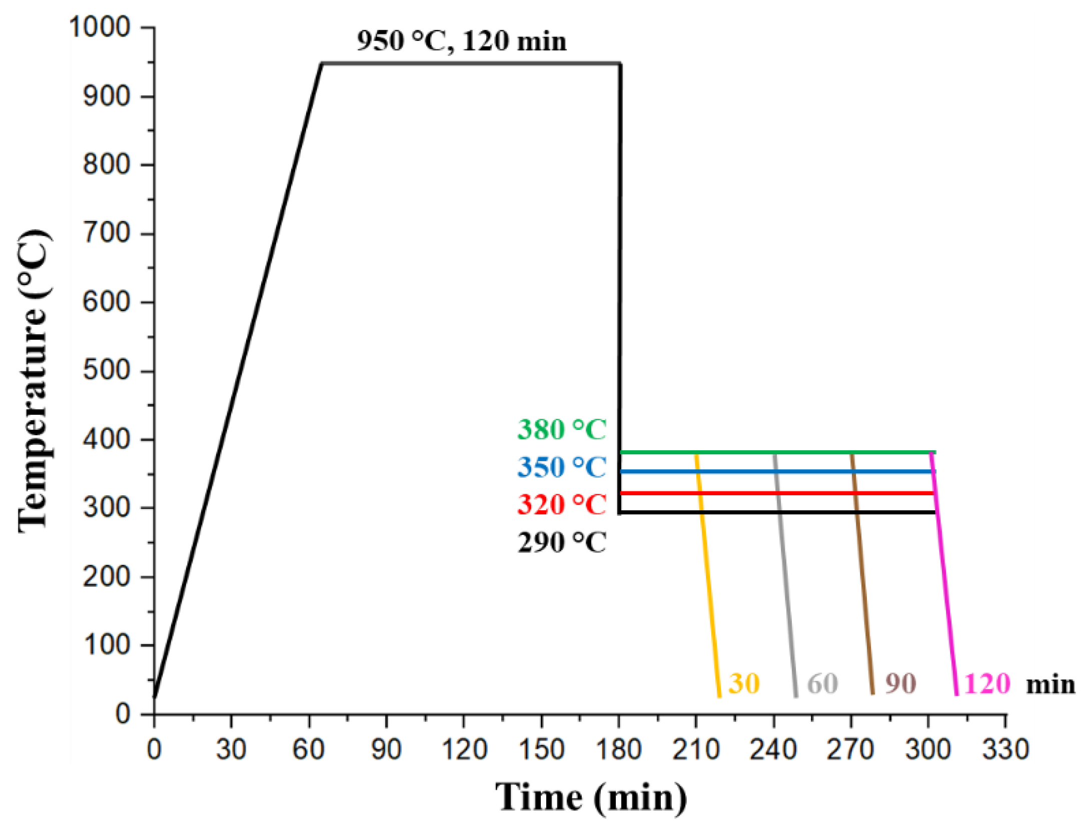
  • Ductile iron is heated to an austenitizing temperature (Tγ), between 850 and 1200 °C, for a sufficient time so as to homogenize the austenitic microstructure.
  • Subsequently, it is rapidly cooled in a molten salt bath to austempering temperature (TA), above the martensitic transformation onset temperature (TMs), between 250 and 450 °C, in order to avoid pearlitic transformation.
  • Afterwards, material is isothermally kept at TA, for a certain austempering time (tA), to allow the formation of an ausferritic matrix. Finally, it is removed from the salt bath and air-cooled to room temperature.
Transformation of ausferritic microstructure takes place upon austempering and is related to the nucleation and growth of ferrite plates within an austenitic matrix. Transformation kinetics is affected by the chemical composition of the melt and heat treatment temperatures as well as the shape, size and distribution of graphite [9]. These austempering phase transformations can be described as a two-stage reaction.
In stage I, known as hardening and represented by reaction (1), the austenite (γ) transforms to a αac, which has a lower carbon solubility than austenite, so the excess of carbon atoms in ferrite diffuse into the surrounding austenite. At this stage, ferrite nucleation is triggered by subcooling from Tγ to TA and happens preferentially at the γ/G interface and austenitic grain boundaries. Thereafter, the growth of this phase occurs in needle-like form promoted by the carbon concentration gradient between αac/γ and γ/G interfaces [10]. The incremental rate of αac needles is regulated via the rate of diffusion of carbon atoms from the αac/γ interface into γ [11]. As transformation proceeds, carbon atoms enrich γ converting it to γhC, increasing its stability and avoiding the transition of γ to martensite (α’) during air quenching [12].
γ → αac + γhC
At stage II, known as embrittlement and represented by reaction (2), produced when the material is subjected to a long isothermal maintenance, γhC slows down αac growth as it becomes saturated with carbon; thus, it continues to increase through the precipitation of iron carbides. For short tA of less than 30 min, ausferritic transformation reaction is not completed, and transformation from γ into α’ occurs. For long tA of more than 2 h, there exists the risk of reaching Stage II, where precipitation of carbides occurs, deteriorating mechanical properties of the casting [13].
γhC → αac + iron carbides
Time elapsed from the end of stage I to the beginning of stage II is known as the processing window [14,15]. The processing window for temperatures close to TMs is smaller because kinetics of ausferritic transformation reaction is higher given the elevated carbon saturation of austenite, which is a consequence of a greater αac needle nucleation [16].
Time and temperature of heat treatment modify phase transformations occurring through austempering since during the ausferritic transformation reaction shearing takes place, in addition to carbon atom diffusion [17]. TA affects mainly the nucleation of αac needles and the diffusion capacity of carbon atoms. For a TA near TMs a higher αac needle nucleation occurs. Nevertheless, carbon diffusion is limited due to the low temperature resulting in an ADI with high hardness and mechanical strength but weak ductility. Meanwhile, at higher temperatures, αac needle nucleation decreases but carbon diffusion is favored [9,18], leading to an ADI with high ductility and poor mechanical strength [19,20].
Industrial use of ADI is complicated when controlling and establishing the variables of production processes, as part and heat treatment design requires a large number of experimental tests in order to validate successful production. Thus, the study of new processing methods, e.g., two-step austempering and usage of mathematical models for predicting final properties and microstructure will contribute to reducing the uncertainty associated with the production, development and implementation of new applications.
Data interpretation has become an important task to be considered within research and development activities of new products. Tools such as the statistical data-driven model (SDDM) enable the prediction and discovery of the repercussions of certain processing variables involved in manufacturing and experimental processes for the validation of prototypes or new products on certain characteristics or properties of interest [21,22,23,24]. This allows a better approach to the design of experiments (DOE) and the search for process optimization based on prediction by statistical analysis. Some related works relying on the SDDM are presented below.
Sivaiah et al. [25] proposed the selection of optimal cutting conditions for 17-4 PH stainless steel turning using the Taguchi method. From statistical analysis results and considering the impact of cutting speed and feed rate, depth of cut and type of coolant, the authors concluded that the optimization of this machining technique is absolutely sustainable, reducing environmental footprint and material waste and enhancing productivity. Montes et al. [26] applied a statistical mathematical model to establish the effect of rotational speed and feed rate on corrosion resistance for dissimilar Al-Cu welds by FSW. By means of this model they determined there is a greater change in corrosion rate as feed rate increases, established the parameters to acquire good quality joints and outlined a microstructural study of their repercussions. Application of statistical analysis in industrial processes such as welding was also carried out by Chandran et al. [27], who proposed laser beam welding parameters with direct influence on tensile and hardness values based on analysis of variance (ANOVA). Analogous to the aforementioned researchers, Choi [28] performed the same kind of statistical analysis method to evaluate the result of using different thicknesses of AZ31 magnesium alloy parts on fatigue crack growth. The author concluded that this procedure could ascertain the impact of part thickness on the characteristics of crack growth as well as on the propagation velocity. Another industrial process implementing ANOVA is parameter optimization in the powder metallurgy process of Al-MoO3 composites, where Sudha et al. [29] sought to obtain the lowest corrosion rate in combination with high compressive strength. They discovered MoO3 reinforcement content has a considerable effect on compressive strength, and corrosion resistance is mostly affected by sintering temperature.
In addition to such statistical studies, artificial intelligence techniques such as fuzzy logic and artificial neural networks are an option for process data analysis as reviewed by Kalpanapriya [30]. These approaches have recently been employed to predict the hardness values in ADI [31,32].
This research provides a novel approach to microstructural studies and their effect on hardness for ADI supported by the statistical data-driven model (SDDM). In this case, ANOVA determines the significant degree of the input variables (time and temperature) for ADI hardness. In addition, if the upper and lower confidence intervals are calculated narrowly, the results of each experiment can be statistically replaced with the mean in each configuration.
Therefore, the prediction of the hardness in ADI is represented by a numerical approximation. The model estimates the hardness for the heat treatments with data experimentation presented in this research, and even it can deal with values outside the DOE domain. In addition, the proposed regression model requires fewer data to predict the hardness in comparison to artificial neural network (ANN) techniques, as the ANN needs an extensive database and a high cost of computation for the training stage. On the other hand, fuzzy logic estimation is based on the human experience; therefore, a unique model for the process is complicated to establish.

2. Materials and Methods

2.1. Heat Treatments

Three samples per heat treatment condition of 20 mm × 20 mm × 10 mm were obtained from a ductile iron profile provided by the company Questum Castings (Santa Catarina, Mexico) of class 100-70-03, according to ASTM A536 [33], with the chemical composition described in Table 1.
Two muffle furnaces were utilized for austenitizing and austempering heat treatments of ductile iron, a Thermo Scientific FD1535M (Facultad de Ingeniería, Arteaga, Mexico) for austenitizing, carried out at 950 °C for 120 min, and a TL-EMISOR furnace (Facultad de Ingeniería, Arteaga, Mexico) for austempering, varying the temperature every 30 °C from 290 to 380 °C for 30, 60, 90 and 120 min, and finally cooling to room temperature. A combination of potassium nitrate (KNO3) and sodium nitrate (NaNO3) salts in a 1:1 ratio was used for austempering heat treatment. Figure 1 illustrates the schematic diagram of heat treatments performed to obtain ADIs.

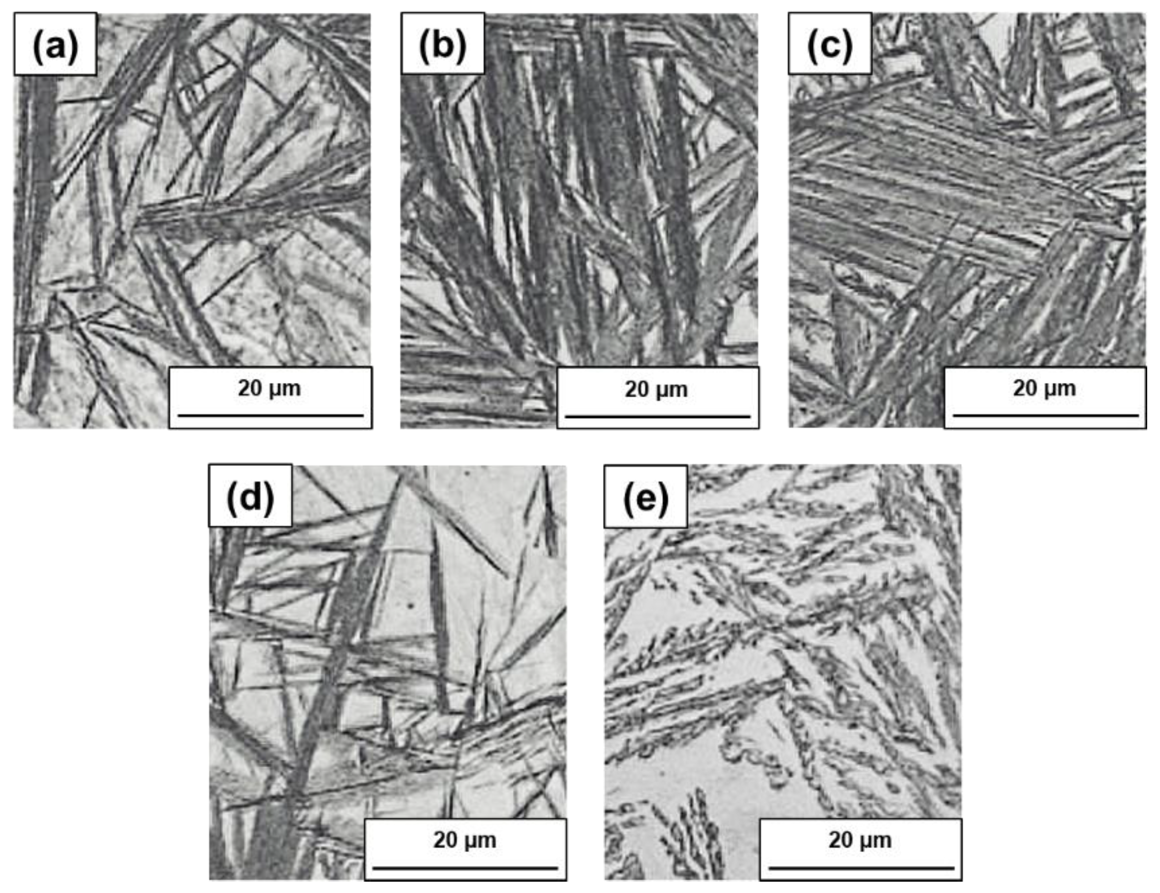
2.2. Microstructural Characterization

On completion of heat treatments, samples were prepared metallographically. Microstructural characterization of ductile iron, before and after heat treatments, was conducted under an Olympus optical microscope (I.T. Saltillo, Saltillo, Mexico) and ImagePro image analyzer (I.T. Saltillo, Saltillo, Mexico). Samples were etched in a solution of nitric acid and 2% ethyl alcohol at room temperature, for approximately 10 s, to reveal microstructure. To quantify the γhc of each sample, 10 micrographs were taken at 500× magnification to guarantee the reliability of results.

2.3. Hardness Tests

Rockwell C hardness measurements were made on a Buehler Macromet 5100 and a diamond tip indenter, under a load of 150 kgf for 10 s on the previously polished surface, as per ASTM E18 standard specification [34], with a distance of 3 mm between each indentation, extending from the center to both sides of the material. A total of 15 hardness measurements were performed for each heat treatment condition.

3. Results and Discussion

3.1. Microstructural Analysis and Hardness

According to the chemical analysis developed by the company Questum Castings, presented in Table 1, C and Si contents are within the recommended composition for ductile iron; notwithstanding, Mn content is slightly high, ranging from 0.2 to 0.7%. While adding this element improves mechanical properties without affecting the machining process, there is a risk of carbide formation for contents above 0.7%. Notably, Mn has a very severe positive segregation, so the addition of copper helps to counteract it. Further, Mn and Cu together enhance the hardenability of the castings, preventing the occurrence of pearlite, which reduces mechanical properties, during severe quenching in the salt bath [35,36].
The microstructure of the metal matrix of ductile iron prior to the austempering heat treatment is completely pearlitic, as shown in Figure 2. This is attributed to the addition of Cu and Mn in ductile iron promoting the appearance of the pearlitic matrix, and together with Sn, the transformation to pearlite is ensured during solidification because it reduces the minimum subcooling for pearlite nucleation [37,38,39]. The nodularity is 96%, and nodule count equals 90 nodules/mm2. The total volume of graphite is 10.33%, and that of the metal matrix is 89.67%.
Microstructures obtained after austempering heat treatments exhibit a characteristic ausferritic metallic matrix composed of αac needles and γhC phase, as seen in Figure 3.
Morphology, distribution, and size of ausferrite depend on the site where nucleation occurs, carbon saturation of austenite during growth and austempering temperature. Figure 4 depicts the different morphologies of the phases found in some samples. Figure 4a shows for the sample treated at 320 °C for 30 min, in a faint gray color, the appearance of α’ between the αac needles. This happens even though the temperature is above the martensitic transformation starting one, since austenite is not completely enriched with carbon, leaving some untransformed austenite, which upon cooling to room temperature is transformed into martensite, in addition to material internal stresses [12]. In Figure 4b it can be noted how in the sample treated at 290 °C for 90 min, αac needles converge at the same nucleation site, giving the appearance of αac needle bundles. Another type of αac needle arrangement consists of clusters, as observed in the sample treated at 320 °C for 90 min in Figure 4c, which is composed of parallel αac needles separated by γhC, similar to results of other researchers [40,41,42,43]. Meanwhile, Figure 4d,e illustrate the two types of αac needles, fine (lower ausferrite) and feathery (upper ausferrite), respectively, within the samples treated at 290 and 380 °C for 60 min, as reported by Putantunda and Olawale [19,44].
The microstructures obtained under all treatment conditions are shown in Figure A1 in Appendix A, demonstrating an increase in the presence and size of γhC blocks caused by an increment in TA. This behavior has been also documented in several investigations and is attributed to carbon atoms diffusing longer distances and stabilizing a greater amount of austenite, resulting in lower nucleation of αac needles [45,46,47]. The TA effect is also evidenced by this figure as it is possible to observe the enlargement and thickening of αac needles as time elapses, with a redistribution of carbon and achieving a transformation of γhC into αac [19,48,49]. Moreover, for the same tA, ferrite inserts become thick when produced at higher temperatures given that the austempering process is highly dependent on the rate of carbon diffusion.
Change in ausferritic morphology is exhibited in Figure 5. At a temperature of 290 °C (Figure 5a) the presence of lower ausferrite indicated by red circles is evident, at 320 °C (Figure 5b) a combination of lower and upper ausferrite can be observed and finally at temperatures of 350 and 380 °C (Figure 5c,d) an all upper ausferritic morphology is indicated by yellow circles. Such a transition in ausferritic morphology is primarily influenced by TA and occurs because at temperatures around TMs the transformation is dominated by αac needle nucleation, and at higher temperatures the transformation is dominated by their growth, as reported by [19,45,50].
Throughout the austempering process, cooling is performed from Tγ to TA with its impact being observed in terms of αac needle nucleation. Figure 6 depicts the microstructural outcome of this cooling, which demonstrates that as TA goes up, there is a limit in αac nucleation and, therefore, a rise in γhC stabilization. At temperatures ranging from 290 to 350 °C, regions that have not been enriched with sufficient carbon to prevent the transformation from γ to α’are detected. As TA increases, the formation of these zones decreases until reaching 380 °C, where they disappear since the diffusion of carbon atoms is facilitated by the effect of temperature. For all 30 min TAs, α’ is found between the αac needles.
Figure 7a shows the γhC quantification for the different heat treatment conditions. It is observed that increasing TA increases the amount of γhC, for a constant time. On the other hand, as tA increases at the same TA there is a maximum in γhC content after which diffusional transformation of γhC to αac is favored. These results are similar to those found by other researchers both in ADI [51,52] and in steel subjected to austempering treatment [53].
The lowest level of γhC is at 30 min of treatment, attributed to the γ low carbon stabilization, so during post-austempering air-cooling, a large part of this γ transforms into α’ [12], as exposed in Figure 6. After 60 min a decrease in γhC is noticed for temperatures of 290 and 320 °C, and for 350 °C this reduction takes place until 120 min, while at 380 °C γhC content stabilizes. This behavior derives from transformation kinetics, i.e., as the TA diminishes, the ausferritic transformation reaction proceeds faster, consuming γhC for αac formation and at possible carbide precipitation [54,55,56]. Figure 7b shows hardness values decreasing as TA increases, consequence of a higher amount of γhC and the change of ausferritic morphology in the metal matrix. A decrease in hardness can also be noticed as tA increases, given that carbon redistribution and coarsening of ausferritic microstructure are present [48,49].

3.2. Mathematical Model

This section introduces the SDDM evaluation of hardness values retrieved from experimentation. In the first analysis, an ANOVA was performed to determine tA and TA effect on sample hardness. For the second analysis, a regression model was used to numerically describe the process and predict hardness values for each tA and TA condition. The third analysis determined the quality of both the proposed regression model and the experimental data through the residual error between them. Experimental data and results must satisfy the following assumptions:
Assumption 1.
The probability distribution (Students’s t) of analyzed data is a normally distributed distribution for small experimental sample sizes as is the case of ADI studied in this research.
Assumption 2.
The alternative hypothesis from ANOVA validates the significance impact of tA and TA on hardness degree of the samples.
Theorem 1.
If the number of samples for each experiment is n < 30 and the confidence intervals in a Student’s t distribution with a significance level α = 0.05 are narrow, then the number of experiments to be statistically analyzed is reduced to the mean y ¯ of each experimental setup.
Proof of Theorem 1.
Two-tailed confidence intervals with a probability α 2 , using the t -distribution for samples smaller than 30 are calculated according to Equation (A1). For the 16 experimental setups in Table A1, 15 hardness tests each were performed, meaning a total of 240 experiments. Given n = 15 and the distribution random variable   t = 2.1448 , the upper and lower bounds are found with a 95% confidence level, i.e., t ( α , n ) . Table A1 sets out the confidence limits quite close to the mean   U i L j ~ y ¯ . All this denotes an acceptable experimental design enabling the report of 240 experiments to be statistically replaced with the mean at each of the 16 configurations. Details of can be seen in Appendix B. □
Figure 8 depicts the normal probability of average hardness versus the percentile sample of each test. A 97.13% linear trend across the distribution suggests an acceptable experimentation for statistical analysis.

3.3. ANOVA

Based on Figure 8 it is possible to implement a Pearson correlation analysis ( r )   to examine the relationship between variable x (time and temperature) and variable y (hardness), involving 1 r 1 . If   r > 0 , y tends to increment as x increments; if r < 0 , and y tends to decrement as x increments. The stronger the linear relationship of x and y , the closer r is to −1 or 1; the weaker the linear relationship, the closer it is to 0. This means that the inversely proportional behavior from tA and TA causes a higher effect of the temperature on the hardness values in comparison to the time effect. This can also be clearly observed in the microstructural results, where the TA modifies the ausferritic morphology, and the tA affects the ausferritic transformation progress. Therefore, the hardness values need to be adjusted according to quality standards requirements. As a consequence, tempering temperatures are recommended. This coefficient is estimated as in Equation (3) and results from Table 2 and Table 3, which list the temperature–time and ADI hardness Pearson correlation, that is, the type of relationship between variables and the kind of increase among them, respectively, in agreement with [56,57].
r = s x y s x s y
where s x and s y are the standard deviations, and s x y the covariance of x and y , correspondingly [57].
ANOVA was conducted to identify the influence of one or more factors on the mean hardness, i.e., whether or not they have a significant effect on the experiment. Similarly, sampling theory seeks to compare the dissimilarities of two or more sample means, based on the assumption that populations have the same variance. It is often necessary to test the hypothesis which assumes that means are equal [56,58]. The significance level α is the probability of rejecting the null hypothesis when it is true and helps us to establish whether the contrast statistic is in the rejection zone or not, for this study and as mentioned in Theorem 1, α = 0.05.
The null hypothesis ( H 0 ) points to the absence of significant differences, produced by the variables, in the phenomenon. This is accepted if:
F c a l c u l a t e d < F c r i t i c a l
The alternative hypothesis ( H i ) states that significant differences do exist in the phenomenon produced by the variables. This hypothesis is accepted if:
F c a l c u l a t e d > F c r i t i c a l  
F c r i t i c a l is attained from the Fisher F distribution conditioned on the degrees of freedom. The statistical factor between sample variances S 1 2 / S 2 2 is considered in this distribution. When ratio is large or small it indicates a huge difference across the variances; conversely, when near 1 it indicates a small difference between analyzed samples. If we have two samples of size N 1 and N 2 , S 1 and S 2 represent the sample variances, respectively, taken from two normal populations with variances σ 1 2 and σ 2 2 . F -statistic is defined as in Equation (4):
F c a l c u l a t e d = S ^ 1 2 σ 1 2 S ^ 2 2 σ 2 2 ,     S ^ n 2 = N n S n 2 N n 1  
Fisher’s F distribution degrees of freedom are calculated as v n = N n 1 .
Such a Fisher statistical distribution is given by Equation (5) according to [50,52]
T = C F ( v 1 2 ) 1 ( v 1 F + v 2 ) ( v 1 + v 2 ) / 2  
with C being a constant dependent on v 1 and v 2 , so the area under the curve equals 1. In the distribution tables, v 1 stands for the degrees of freedom in the numerator ( v R y v C ) and v 2 for those in the denominator ( v E ) [56,58]. Assuming population variances σ 1   = σ 2 or H 0 , F c a l c u l a t e d is obtained from:
S R 2 S E 2   and   S C 2 S E 2  
Variation among treatments is as follows:
V R = b i = 1 a ( X ¯ i X T ̿ ) 2
where a is the number of rows, b the number of columns,   X ¯ i   the average of the rows and X T ̿ the total average. Block-to-block variation is described as:
V C = a i = 1 b ( X ¯ j X T ̿ ) 2
where X ¯ j is the average of the columns. The total data variance is defined as:
V = ( x i , j X T ̿ ) 2
with x i , j representing the values from Table A1. Therefore, the residual variance of collected data becomes:
V E = V V R V C  
The mean square between treatments is:
S R 2 = V R a 1  
while inter-block mean square equals:
S C 2 = V C b 1  
and the mean square between residuals is expressed:
S E 2 = V E ( a 1 ) ( b 1 )
in which S R = S T e m p e r a t u r e and S C = S T i m e .
From Table 4, H 1 is validated for ADI treatment results, meaning that F c a l c u l a t e d     F c r i t i c a l for TA and tA, i.e., there is an effect of these two variables on sample hardness degree.
Probability displayed in Table 4 variance analysis comes from the right tail of F distribution corresponding to the F c a l c u l a t e d value for treatments and blocks with their respective degrees of freedom. This probability is computed via the Excel function distr.F.CD ( F c a l c u l a t e d , treatment or block degrees of freedom ( d o f ), error degrees of freedom).

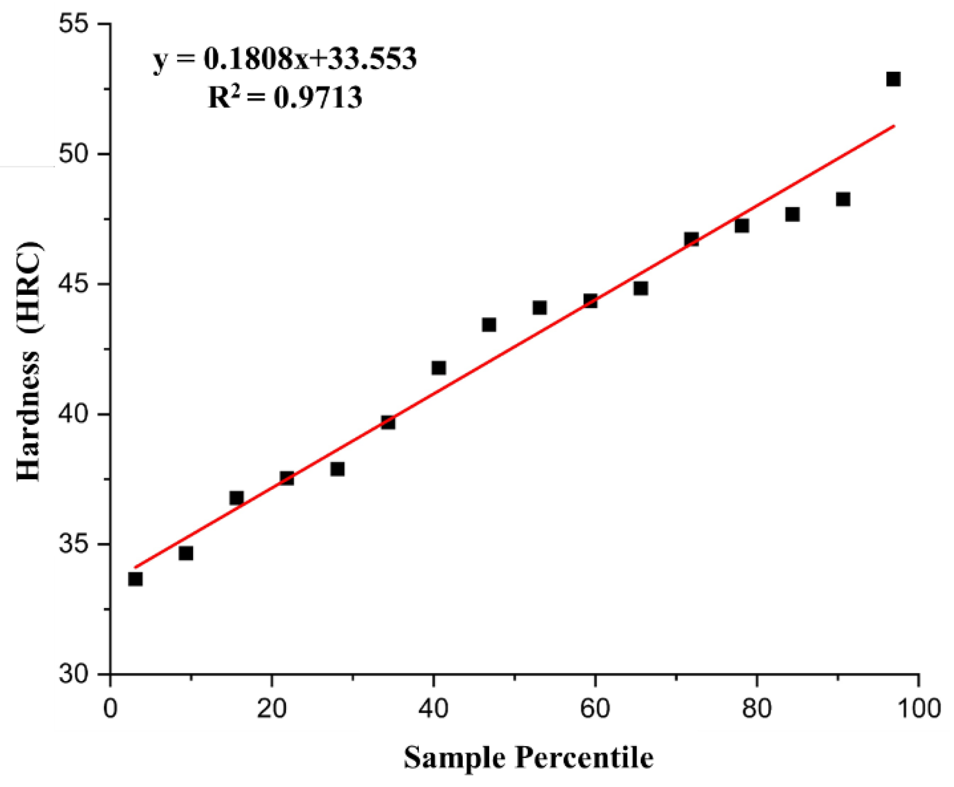
3.4. Least Squares Regression

The model to approximate the hardness value in terms of the austempering time and temperature is obtained through a power equation based on the least square method as is presented below:
Corollary 1.
When the analyzed data set exhibits substantial errors, the use of polynomial interpolation is inappropriate in view of the unsatisfactory prediction level at intermediate values. In contrast, an approximation of a general trend of the data, by a power regression, is more useful for minimizing the sum of residual squared errors between y   m e a s u r e d and y   c a l c u l a t e d , estimated with the model.
The squared error sum is presented in Equation (14) as reported in [58]:
S r = i = 1 n e i 2 = ( y ,   m e a s u r e d y c a l c u l a t e d ) 2
A regression model with a power equation is proposed as in Equation (15), in which a hardness function in terms of temperature and time is provided for ADI heat treatment:
D = a 0 T A a 1 t A a 2 ln ( D ) = ln ( a 0 ) + a 1 ln ( T A ) + a 2 ln ( t A )
where a 0 ,   a 1 , a 2 are the coefficients for describing the function of this process and D is the hardness. Using the properties of natural logarithms, Equation (15) can be linearized. In a multiple regression, the linearized power equations are the most suitable to fit experimental data. Upon applying Equations (14) and (15), the sum of the quadratic errors is determined for the particular case of the study carried out in this research.
S r = i = 1 n e i 2 = i = 1 n [ ln ( D i ) ln ( a 0 ) a 1 ln ( T A i ) a 2 ln ( t A i ) ] 2
To compute the coefficient values, Equation (16) is derived with respect to each coefficient, recalling that S r a 0 , S r a 1 ,   S r a 2 must equal zero to minimize the error between measured and calculated data in Equation (14). Once the parameters are estimated, the following model emerges:
D = e 10.393 T A 1.0599 t A 0.1173

3.5. Quantification of Error in Regressions

In accordance with [57,59], the magnitude of residual error associated with the dependent variable before regression is
S t = i = 1 n ( y ,   m e a s u r e d y m e a n ) 2
where St is the total sum of squares around dependent variable y mean. Subsequent to regression, S r   is estimated, which represents the sum of squares of the residuals around the regression function. This characterizes the residual error remaining after regression. The difference between these two summations, S t S r , quantifies error through data description in terms of a straight line rather than an average value. Because the magnitude of this quantity depends on the scale, the difference is normalized to S t to obtain:
r 2 = S t S r S t
Here, r2 is known as the coefficient of determination, and r is the correlation coefficient ( r 2 ). A perfect data fit, Sr = 0 and r = r2 = 1, indicates that function explains 100% of data variability. If r = r2 = 0 and St = Sr the fit does not imply any improvement.
Standard error is formulated as in Equation (18). Said number is divided by n ( m + 1 ) since ( m + 1 ) coefficients drawn from the data, a 0 , a 1 , , a m , were employed to calculate   S r ; m + 1 degrees of freedom are lost. Briefly it can be stated that:
S y / x = S r n ( m + 1 )
where m + 1 = total degrees of freedom and n = number of experiments.
Adjusted coefficient of determination r 2 a d j u s t e d is used in multiple regression to observe the intensity or effectiveness of independent variables (TA and tA) with regard to the dependent one ( D ). The computation of r 2 a d j u s t e d is set out in Equation (21):
r 2 a d j u s t e d = 1 n 1 n m + 1 ( 1 r 2 )
Table 5 reveals the direct relationship of hardness degree and the magnitude of T A and t A . Based on the coefficient of determination r2, it is established that the proposed power equation model is able to describe 95.2% of the phenomenon uncertainty. As per r 2 o d j u s t e d , contemplated variables occupy 94.46% of model effectiveness, which means that there are some other factors that impact the remaining 5.54% of the phenomenon. The power equation model has an estimation error of ±1.2845.
Theorem 2.
If the variability of the experimental data r2 is ~ 1 and standard error converges towards zero S y / x 0 , then the upper ( U ) and lower ( L ) interval values of the power regression coefficients   a 0 , a 1 , a 2   in Equation (15), evaluated at a 95% confidence level, converge to values near each other in very close intervals.
Proof of Theorem 2.
For the regression model (17), the coefficient of determination   r 2 = 95.20 % , the standard error   S y / x = 1.2845   and the values of upper U and lower L intervals are determined by Equations (A5) and (A6), Results are listed in Table A3 for each coefficient a 0 ,   a 1 , a 2 . Details can be noticed in Appendix C. □
Remark 1.
On the basis of Theorem 2, the Equation (17) model holds for increasing numbers of experimental data and in domains outside tested data. This prevents excessive experimentation.
Figure 9 compares the experimental results and those estimated by the model demonstrating the impact of T A and t A on hardness. Model results are reliable at least in the experimental range.
Figure 10 depicts the surface simulation of the data reconstructed by the proposed model for each T A and t A hardness value. For the domain 30 <   t A   < 60 and 290 <   T A   < 315, the highest hardness values are attained, ascribed to the presence of α’ and lower ausferrite, respectively, as 53.78 HRC was yielded from the application of a treatment at 290 °C for 30 min. In the case of the domain 70 <   t A   < 120 and 340 <   T A   < 380, the lowest hardness values are achieved, a consequence of a coarsening of the microstructure and a higher amount of γhC, correspondingly. In other words, the higher the temperature, the lower the hardness and vice versa, and the longer the treatment time, the lower the hardness and vice versa. This behavior has also been documented by other authors [60,61,62], and these materials exhibited excellent wear resistance and tensile strength properties for their possible application as high-performance components.

4. Conclusions

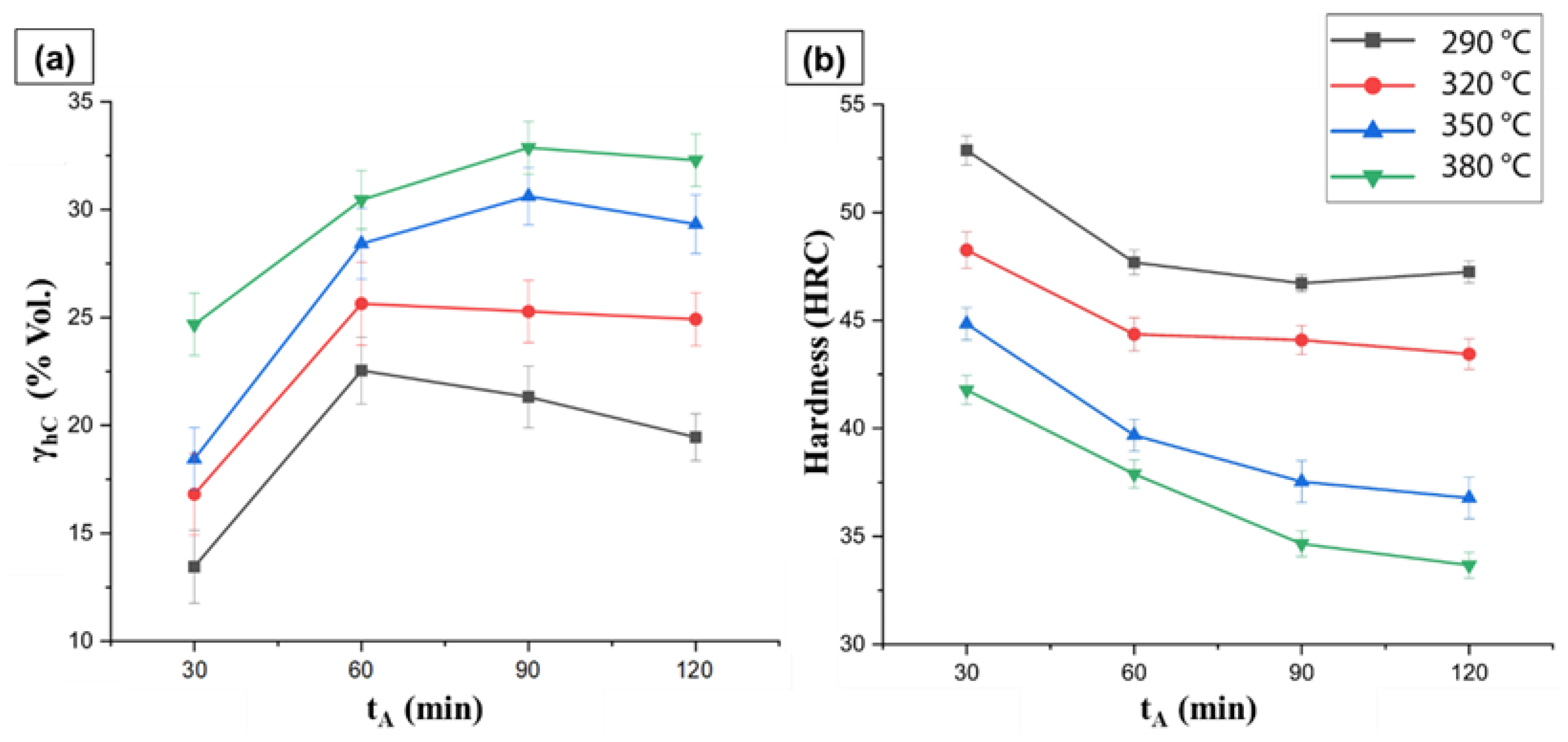
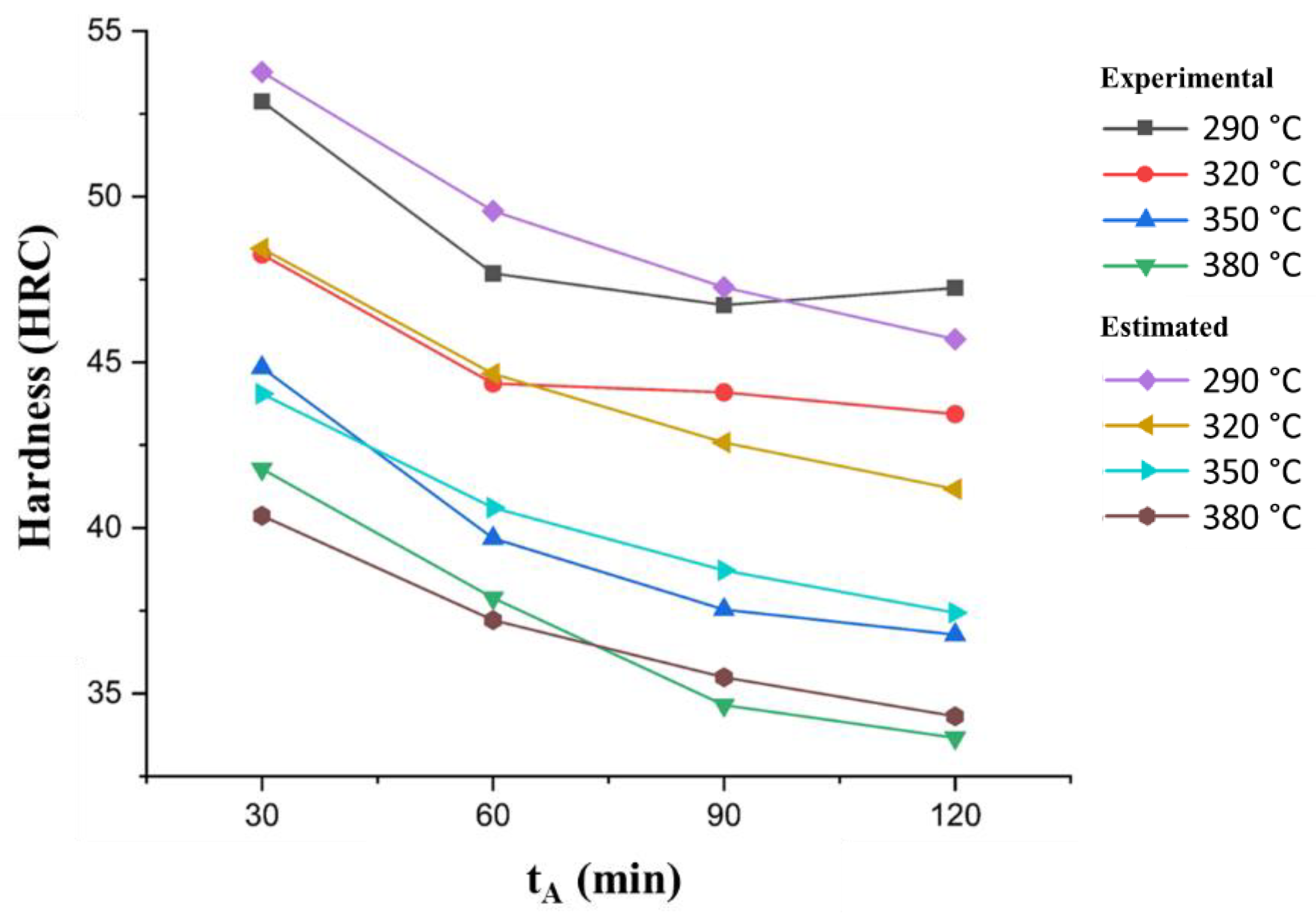
  • The effect of austempering time and temperature on hardness shows an inversely proportional behavior, which was verified by the SDDM. This relationship is attributed to the microstructural characteristics acquired during the heat treatment.
  • ANOVA quantifies the statistical influence of the time and temperature of tempering on the degree of hardness for ADI samples. The correlation study shows there is a strong inverse relationship between hardness and temperature, i.e., this is consistent with the microstructural characteristics found in the treatment. In the power regression model indicates that the multiple correlation between variables is around 97.57%, the adjusted coefficient of determination is 94.46% and the standard error is ±1.2845.
  • By means of ANOVA, it was possible to quantify the significant influence of austempering time and temperature on the hardness degree of ductile iron samples. Multiple correlation among variables is about 97%. The correlation study shows there is a strong inverse relationship between hardness and temperature, i.e., the higher temperature lowered the hardness and vice versa. This is consistent with the microstructural characteristics found in the treatment.
  • A model representing the numerical response of hardness degree as a function of time and temperature in the austempering treatment of ductile irons is presented. Model variability is 95.20% in the face of uncertainties, and according to Theorem 2, the proposed model can avoid excessive experimentation for this process. Additionally, quality of the data and model was analyzed, and confidence intervals were defined for both cases.
Future work including the effect of alloying elements on hardness in a new mathematical model is being considered.

Author Contributions

Conceptualization, N.A.R.-R., C.R.M.-V. and F.A.M.-G.; Methodology, N.A.R.-R. and C.R.M.-V.; Validation, J.S.G.-V. and J.C.O.-C.; Formal Analysis, J.G.-C., D.G.-N., O.G.-C. and J.F.M.-V.; Investigation, F.A.M.-G. and N.A.R.-R.; Resources, C.R.M.-V.; Data Curation, J.G.-C. and D.G-N.; Writing—Original Draft Preparation, J.G.-C., N.A.R.-R. and F.A.M.-G.; Software, J.G.-C. and O.G.-C.; Writing—Review and Editing, J.S.G.-V. and C.R.M.-V.; Supervision, J.G.-C. and J.F.M.-V. All authors have read and agreed to the published version of the manuscript.

Funding

This research received no external funding.

Data Availability Statement

The research data and methods used in the investigation are presented in sufficient detail in the paper to allow other researchers to reproduce the work.

Acknowledgments

We gratefully acknowledge CONACYT México, Tecnológico Nacional de México, Universidad Autónoma de Coahuila and Questum Casting for the support in this investigation.

Conflicts of Interest

The authors declare no conflict of interest.

Appendix A

Figure A1. Microstructures of ADI treated under different heat treatment conditions.
Metals 12 00676 g0a1

Appendix B. Confidence Interval for Samples n < 30

For this investigation, the number of samples n in each experimental setup in Table A1 was less than 30. In this case, the t distribution was utilized to obtain the confidence levels. Said t distribution is a modification of the normal distribution. When the number of samples in each experimental configuration n tends to be small, distribution tends to be flatter, and wider and more conservative confidence intervals are derived. On the other hand, when n becomes larger, t distribution converges to normal. Two-tailed confidence intervals via t distribution for samples smaller than 30 were computed from Equation (A1) and are in agreement with [56,58]:
y ¯ s y n t α 2 , n 1 < μ < y ¯ + s y n t α 2 , n 1
where y ¯ is the sample mean, s y the sample standard deviation, μ the population mean, n the number of samples, α the significance level and t the standard random variable of the distribution for a probability α 2 .
Confidence intervals arise from Equation (A1) as in Table A1, with α = 0.05 ; that is, upper and lower limits have a 95% confidence level given n = 15 and t = 2.1448. Consequently, in each experiment configuration, these limits are quite close to the mean. The variable t   represents the two-tailed inverse S t u d e n t s   distribution and relies on the significance level and the   n 1 degrees of freedom; in Excel it is found with the function inv.t.2c (α, n − 1).
Table A1. Results of the statistical analysis for the proposed hardness estimation regression model.
TA (°C) t A ( min ) Hardness (Mean)Sample Std. Dev.Lower Limit (Li)Upper Limit (Ui)
2903052.880.704352.490053.2700
6047.690.576847.367348.0061
9046.730.413146.497946.9554
12047.250.527646.954547.5389
3203048.260.880647.772348.7477
6044.360.794443.920144.7999
9044.090.693343.709444.4773
12043.440.736643.032143.8479
3503044.840.774444.411145.2689
6039.690.758839.265140.1056
9037.531.005536.976538.0901
12036.780.993036.230137.3299
3803041.780.687941.399142.1609
6037.890.671737.514738.2587
9034.650.609334.315934.9907
12033.670.623033.321734.0117

Appendix C. Statistical Aspects of Least Squares Theory

To assess the quality and reliability of the models, confidence intervals were estimated, but it is necessary to define the following concepts.
In a general way, K = coefficient matrix, { K } 1   = coefficient matrix inverse, X = vector of variables or unknowns, Y = right hand side vector and t = standard random variable of the t distribution for a probability of   α 2 .
Furthermore, s ( a i , j )   = standard error of coefficient   a i , j = v a r ( a i , j ) , with a i , j being an element of the diagonal of the inverse matrix { K } 1 .
The least squares method for linear forms formulates the following matrix system:
{ K } { X } = { Y }
so that the solution to the system is:
{ K } 1 { K } { X } = { K } 1 { Y }  
Consistent with [52], it is possible to prove that the terms on the diagonal of { K } 1 matrix give the variances of a n :
v a r ( a i , j ) = { K } 1 i , j S y / x 2     s ( a i , j ) = T y p i c a l   e r r o r = v a r ( a i , j )  
For our present purposes, we illustrate how they are applied to develop confidence intervals for y -axis intersection. Lower and upper bounds for the y -intercept can be found as below (Equation (A5) for lower bound L and Equation (A6) for upper bound U ):
L = a n t α 2 , n m + 1 s ( a i , j 1 )
U = a n + t α 2 , n m + 1 s ( a i , j 1 )
s t . t = a n v a r ( a i , j 1 )
The statistic t is computed as in Equation (A7). For the critical value of   t in Excel, the INV.T.2C function is used (probability = significance level; degrees of freedom =   n ( m + 1 ) ) .
Probability values for each coefficient in Table A1 come from the two-tailed S t u d e n t s   t -distribution and depend on the | statistic   t | of each coefficient and its degrees of freedom = n ( m + 1 ) . Probability is available in Excel with the function distr.t.2c( | statistic   t |   , n ( m + 1 ) ).
We then evaluated and examined the confidence intervals of the models provided in Table A2 and Table A3, where for   m + 1 = 3 , n = 16 , and α = 0.05 , we have   t = 2.1604 .
Table A2. Confidence intervals of regression model coefficients.
Coefficients v a r ( a i 1 ) Standard
Error
Statistic   t Probability L U
l n ( a 0 ) 10.39300.19120.437323.76824.25954 × 10−129.448411.3377
a 1 −1.05990.00560.0745−14.21972.66365 × 10−9−1.2209−0.8989
a 2 −0.11730.000210.0144−8.13111.8708 × 10−6−0.1485−0.0861
In the model statistical analysis, confidence intervals for the coefficients ( L , U ) are extremely tight with 95% confidence. This suggests that if the study were implemented with more data, they would fall around the marked intervals and could further narrow the interval and raise r 2 . However, the possibility of their convergence radius reaching its limit also exists, and excessive experimentation would just be more expensive with no improvement in results.
Table A3. Linear and power model comparison in a random domain.
iT (°C)t (min)PowersLinearDifference
135016835.989433.87962.1098
24295233.283631.64301.6406
33017446.490647.22790.7373
43825837.160437.51540.3550
54245833.270931.88131.3896
64428130.613427.80892.8045
72133672.988361.771711.2166
824612554.142850.93003.2127
93584740.800041.52770.4839
1033114538.847838.08610.6808
Besides the   D = e 10.393 T 1.0599 t 0.1173 model, another linear model D = 92.9394 0.1341 T 0.0721 t was calculated which, despite having statistically favorable results, was slightly inferior to the power one. With these two models, 10 totally random simulations were created in a wider domain than that performed in the experimentation, where results of both models were very similar. Because of the nature of the function, the power model was also chosen over a polynomial, since the latter would never yield negative values in any range of values. Moreover, due to the exponents a1 and a2, values t ≥ 0 and T ≥ 0 would be accepted which is consistent with reality.

References

  1. Du, Y.; Wang, X.; Zhang, D.; Wang, X.; Ju, C.; Jiang, B. A superior strength and sliding-wear resistance combination of ductile iron with nanobainitic matrix. J. Mater. Res. Technol. 2021, 11, 1175–1183. [Google Scholar] [CrossRef]
  2. Artola, G.; Gallastegi, I.; Izaga, J.; Barreña, M.; Rimmer, A. Austempered ductile iron (ADI) alternative material for high-performance applications. Int. J. Metalcast. 2017, 11, 131–135. [Google Scholar] [CrossRef]
  3. Eraslan, D.; Balcı, A.; Çetin, B.; Ucak, N.; Çiçek, A.; Yılmaz, O.D.; Davut, K. Machinability evaluations of austempered ductile iron and cast steel with similar mechanical properties under eco-friendly milling conditions. J. Mater. Res. Technol. 2021, 11, 1443–1456. [Google Scholar] [CrossRef]
  4. Larumbe, L.H.; Delgado, E.H.; Alvarez-Vera, M.; Villanueva, P.P. Forming process using austempered ductile iron (ADI) in an automotive Pitman arm. Int. J. Adv. Manuf. Technol. 2017, 91, 569–575. [Google Scholar] [CrossRef]
  5. Wang, B.; Qiu, F.; Barber, G.C.; Pan, Y.; Cui, W.; Wang, R. Microstructure, wear behavior and surface hardening of austempered ductile iron. J. Mater. Res. Technol. 2020, 9, 9838–9855. [Google Scholar] [CrossRef]
  6. Fraś, E.; Górny, M.; Lopez, H. Thin Wall Ductile Iron Castings as Substitutes for Aluminium Alloy Castings. Arch. Metall. Mater. 2014, 59, 459–465. [Google Scholar] [CrossRef]
  7. Goergen, F.; Mevissen, D.; Masaggia, S.; Veneri, E.; Brimmers, J.; Brecher, C. Contact Fatigue Strength of Austempered Ductile Iron (ADI) in Gear Applications. Metals 2020, 10, 1147. [Google Scholar] [CrossRef]
  8. Chen, X.R.; Zhai, Q.J.; Dong, H.; Dai, B.H.; Mohrbacher, H. Molybdenum alloying in cast iron and steel. Adv. Manuf. 2020, 8, 3–14. [Google Scholar] [CrossRef] [Green Version]
  9. Meier, L.; Hofmann, M.; Saal, P.; Volk, W.; Hoffmann, H. In Situ Measurement of Phase Transformation Kinetics in Austempered Ductile Iron. Mater. Charact. 2013, 85, 124–133. [Google Scholar] [CrossRef]
  10. Guilemany, J.M.; Llorca, N. Mechanism of bainitic transformation in compacted graphite cast irons. Metall. Trans. A 1990, 21, 895–899. [Google Scholar] [CrossRef]
  11. Rouns, T.N.; Rundman, K.B. Constitution of Austempered ductile Iron and the Kinetics of Austempering. AFS Trans. 1987, 95, 851–887. [Google Scholar]
  12. Sikora, J.; Rivera, G.; Biloni, H. Metallographic study of the eutectic solidification of gray, vermicular and nodular cast iron. In Proceedings of the 29th Annual Conference of Metallurgists, Hamilton, ON, Canada, 27–29 August 1990; pp. 280–288. [Google Scholar]
  13. Yescas, M.A.; Bhadeshia, H.K.D.H.; MacKay, D.J. Estimation of the amount of retained austenite in austempered ductile irons using neural networks. Mater. Sci. Eng. A 2013, 311, 162–173. [Google Scholar] [CrossRef]
  14. Zahiri, S.H.; Pereloma, E.V.; Davies, C.H.J. Model for prediction of processing window for austempered ductile iron. Mater. Sci. Technol. 2002, 18, 1163–1167. [Google Scholar] [CrossRef]
  15. Bayati, H.; Elliott, R. The Concept of an Austempered Heat Treatment Processing Window. Inter. J. Cast Metals Res. 1999, 11, 413–417. [Google Scholar] [CrossRef]
  16. Cekic, O.E.; Sidjanin, L.; Rajnovic, D. Austempering kinetics of Cu-Ni alloyed austempered Ductile Iron. Met. Mater. Int. 2014, 20, 1131–1138. [Google Scholar] [CrossRef]
  17. Ławrynowicz, Z. Ausferritic or bainitic transformation in ADI. Adv. Mater. Sci. 2014, 13, 9–18. [Google Scholar] [CrossRef] [Green Version]
  18. Putatunda, S.K. Comparison of the mechanical properties of austempered ductile cast iron (ADI) processed by conventional and step-down austempering process. Mater. Manuf. Processes 2010, 25, 749–757. [Google Scholar] [CrossRef]
  19. Panneerselvama, S.; Martis, C.J.; Putatunda, S.K.; Boileau, J.M. An investigation on the stability of austenite in Austempered Ductile Cast Iron (ADI). Mater. Sci. Eng. 2015, 626, 237–246. [Google Scholar] [CrossRef]
  20. Pereira, L.N.D.G.; Medeiros, R.G.D.C.; Freitas, P.G.M.D.; Silva, C.F.D.; Silva, L.M.D.; Leal, R.H. Microstructural Evaluation of an Austempered Cast Iron Alloy. Mater. Res. 2022, 25. [Google Scholar] [CrossRef]
  21. Heshmat, M.; Adel, M. Investigating the effect of hot air polishing parameters on surface roughness of fused deposition modeling PLA products: ANOVA and regression analysis. Prog. Addit. Manuf. 2021, 6, 679–687. [Google Scholar] [CrossRef]
  22. Jha, P.; Kumar, D.; Mishra, V.K. Development of mathematical models to predict the density and hardness of Fe-ZrO2 composites. Adv. Mater. Process. Technol. 2021, 7, 1–15. [Google Scholar] [CrossRef]
  23. Leonzio, G. ANOVA analysis of an integrated membrane reactor for hydrogen production by methane steam reforming. Int. J. Hydrogen Energy 2019, 44, 11535–11545. [Google Scholar] [CrossRef]
  24. Nandagopal, K.; Kailasanathan, C. Analysis of mechanical properties and optimization of gas tungsten arc welding (GTAW) parameters on dissimilar metal titanium (6Al4V) and aluminium 7075 by taguchi and ANOVA techniques. J. Alloys Compd. 2016, 682, 503–516. [Google Scholar] [CrossRef]
  25. Sivaiah, P.; Chakradhar, D. Modeling and optimization of sustainable manufactu- ring process in machining of 17-4 PH stainless steel. Measurement 2019, 134, 142–152. [Google Scholar] [CrossRef]
  26. Montes-Gonzaález, F.A.; Rodriáguez-Rosales, N.A.; Ortiz-Cuellar, J.C.; Muñiz-Valdez, C.R.; Goámez-Casas, J.; Galindo-Valdeás, J.S.; Goámez-Casas, O. Experimental analysis and mathematical model of FSW parameter effect on the corrosion rate of Al 6061-t6-Cu C11000 joints. Crystal 2021, 11, 294. [Google Scholar] [CrossRef]
  27. Chandran, S.; Rajesh, R.; Anand, M.D. Analysis of mechanical properties and optimization of laser beam welding parameters on dissimilar metal titanium (Ti6Al4V) and aluminium (A6061) by factorial and ANOVA techniques. Mater. Today Proc. 2021, 42, 508–514. [Google Scholar] [CrossRef]
  28. Choi, S.S. Evaluating the effect of specimen thickness on fatigue crack growth in AZ31 alloy using ANOVA. J. Korean Soc. Manufact. Process Eng. 2020, 19, 9–16. [Google Scholar] [CrossRef]
  29. Sudha, G.; Stalin, B.; Ravichandran, M. Optimization of powder metallurgy parameters to obtain low corrosion rate and high compressive strength in Al-MoO3 composites using SN ratio and ANOVA analysis. Mater. Res. Express 2019, 6, 096520. [Google Scholar] [CrossRef]
  30. Kalpanapriya, D.; Pandian, P. Fuzzy hypothesis testing of ANOVA model with fuzzy data. Int. J. Mod. Eng. Res. 2012, 2, 2951–2956. [Google Scholar]
  31. Savangouder, R.V.; Patra, J.C.; Bornand, C. Artificial neural network-based modeling for prediction of hardness of austempered ductile iron. In Proceedings of the International Conference on Neural Information Processing, Sydney, Australia, 12–15 December 2019; pp. 405–413. [Google Scholar]
  32. Savangouder, R.V.; Patra, J.C.; Bornand, C. Prediction of hardness of austempered ductile iron using enhanced multilayer perceptron based on chebyshev expansion. In Proceedings of the International Conference on Neural Information Processing, Sydney, Australia, 12–15 December 2019; pp. 414–422. [Google Scholar]
  33. ASTM A536-84; Standard Specification for Ductile Iron Castings. ASTM International: West Conshohocken, PA, USA, 2019.
  34. ASTM E8/E8M-21; Standard Test Methods for Tension Testing of Metallic Materials. ASTM International: West Conshohocken, PA, USA, 2021.
  35. Čatipović, N.; Živković, D.; Dadić, Z. The effect of Molybdenum and Manganese on the Mechanical Properties of Austempered Ductile Iron. Teh. Vjesn. 2018, 25, 635–642. [Google Scholar]
  36. Lacaze, J.; Sertucha, J. Effect of Cu, Mn and Sn on pearlite growth kinetics in as-cast ductile irons. Int. J. Cast Metals Res. 2016, 29, 74–78. [Google Scholar] [CrossRef] [Green Version]
  37. Lacaze, J.; Sertucha, J. Effect of tin on the phase transformations of cast irons. J. Phase Equilib. Diffus. 2017, 38, 743–749. [Google Scholar] [CrossRef] [Green Version]
  38. Lacaze, J.; Sertucha, J.; Larrañaga, P.; Suárez, R. Combined Effects of Copper and Tin at Intermediate Level of Manganese on the Structure and Properties of As-Cast Nodular Graphite Cast Iron. Arch. Metall. Mater. 2017, 62, 825–831. [Google Scholar] [CrossRef] [Green Version]
  39. Hegde, A.; Sharma, S. Machinability study of manganese alloyed austempered ductile iron. J. Braz. Soc. Mech. Sci. Eng. 2018, 40, 338. [Google Scholar] [CrossRef]
  40. Chawla, V.; Batra, U.; Puri, D.; Chawla, A. To Study the effect of Austempering Temperature on Fracture Behaviour of Ni-Mo Austempered Ductile Iron (ADI). J. Miner. Mater. Charact. Eng. 2008, 7, 307–316. [Google Scholar] [CrossRef]
  41. Krzyńska, A.; Kochanski, A. Properties and Structure of High-Silicone Austempered Ductile Iron. Arch. Foundry Eng. 2014, 14, 91–94. [Google Scholar] [CrossRef]
  42. Konečná, R.; Nicoletto, G.; Fintová, S.; Bubenko, L. Threshold for fatigue crack growth and crack paths in heat treated nodular cast iron. In Proceedings of the 4th International Conference of Crack Paths, Gaeta, Italy, 19–21 September 2012; pp. 385–392. [Google Scholar]
  43. Yi, P.; Guo, E.; Wang, L.; Feng, Y.; Wang, C. Microstructure and mechanical properties of two-step Cu-alloyed ADI treated by different second step austempering temperatures and times. China Foundry 2019, 16, 342–351. [Google Scholar] [CrossRef] [Green Version]
  44. Olawale, J.O.; Oluwasegun, K.M. Austempered Ductile Iron (ADI): A Review. Mater. Perform. Charact. 2016, 5, 289–311. [Google Scholar] [CrossRef]
  45. Cruz Ramírez, A.; Colin García, E.; Chávez Alcalá, J.F.; Téllez Ramírez, J.; Magaña Hernández, A. Evaluation of CADI Low Alloyed with Chromium for Camshafts Application. Metals 2022, 12, 249. [Google Scholar] [CrossRef]
  46. Parhad, P.; Likhite, A.; Bhatt, J.; Peshwe, D. Optimization of isothermal transformation period for Austempered Ductile Iron. Metall. Foundry Eng. 2018, 43, 313. [Google Scholar] [CrossRef]
  47. Balos, S.; Rajnovic, D.; Dramicanin, M.; Labus, D.; Eric-Cekic, O.; Grbovic-Novakovic, J.; Sidjanin, L. Abrasive wear behaviour of ADI material with various retained austenite content. Int. J. Cast Metals Res. 2016, 29, 187–193. [Google Scholar] [CrossRef]
  48. Landesberger, M.; Koos, R.; Hofmann, M.; Li, X.; Boll, T.; Petry, W.; Volk, W. Phase Transition Kinetics in Austempered Ductile Iron (ADI) with Regard to Mo Content. Materials 2020, 13, 5266. [Google Scholar] [CrossRef]
  49. Li, X.; Wagner, J.N.; Stark, A.; Koos, R.; Landesberger, M.; Hofmann, M.; Fan, G.; Gan, W.; Petry, W. Carbon Redistribution Process in Austempered Ductile Iron (ADI) During Heat Treatment—APT and Synchrotron Diffraction Study. Metals 2019, 9, 789. [Google Scholar] [CrossRef] [Green Version]
  50. Abioye, A.; Atanda, P.; Abioye, O.; Afolalu, A.; Dirisu, J. Microstructural Characterization and Some Mechanical Behaviour of Low Manganese Austempered Ferritic Ductile Iron. Int. J. Appl. Eng. Res. 2017, 12, 14435–14441. [Google Scholar]
  51. Wang, B.; Barber, G.C.; Tao, C.; Sun, X.; Ran, X. Characteristics of tempering response of austempered ductile iron. J. Mater. Res. Technol. 2018, 7, 198–202. [Google Scholar] [CrossRef]
  52. Akinribide, O.J.; Olusunle, S.O.O.; Akinwamide, S.O.; Babalola, B.J.; Olubambi, P.A. Impact of heat treatment on mechanical and tribological behaviour of unalloyed and alloyed ductile iron. J. Mater. Res. Technol. 2021, 14, 1809–1819. [Google Scholar] [CrossRef]
  53. Parzych, S.; Dziurka, R.; Goły, M.; Kulinowski, B. Effect of austempering temperature on the microstructure and retained austenite of cast bainitic steel used for frogs in railway crossovers. Arch. Metall. Mater. 2020, 4, 1463–1468. [Google Scholar]
  54. Sellamuthu, P.; Samuel, D.G.; Dinakaran, D.; Premkumar, V.P.; Li, Z.; Seetharaman, S. Austempered Ductile Iron (ADI): Influence of Austempering Temperature on Microstructure, Mechanical and Wear Properties and Energy Consumption. Metals 2018, 8, 53. [Google Scholar] [CrossRef] [Green Version]
  55. Cisneros, M.; Campos, R.; Castro, M.; Pérez, M. Austempering kinetics in Cu-Mo alloyed ductile iron: A diatrometric study. Adv. Mater. Res. 1997, 4, 415–420. [Google Scholar] [CrossRef]
  56. Spiegel, M.R.; Stephens, L.J. Estadística, 6th ed.; Mc Graw Hill Global Education Holdings: New York, NY, USA, 2018. [Google Scholar]
  57. Montgomery, D.C. Diseño y Análisis de Experimentos, 2nd ed.; Limusa Wiley: Mexico City, Mexico, 2004. [Google Scholar]
  58. Spiegel, M.R.; John, J.; Srinivasan, R. Probabilidad y Estadística, 4th ed.; Mc Graw Hill: New York, NY, USA, 2013. [Google Scholar]
  59. Chapra, S.C.; Canale, R.P.; Ruiz, R.S.G. Métodos Numéricos Para Ingenieros, 7th ed.; Mc Graw Hill Education: New York, NY, USA, 2015; pp. 372–375. [Google Scholar]
  60. Chiniforush, E.A.; Rahimi, M.A.; Yazdani, S. Dry sliding wear of Ni alloyed austempered ductile iron. China Foundry 2016, 13, 361–367. [Google Scholar] [CrossRef] [Green Version]
  61. Bendikiene, R.; Ciuplys, A.; Cesnavicius, R.; Jutas, A.; Bahdanovich, A.; Marmysh, D.; Nasan, A.; Shemet, L.; Sherbakov, S. Influence of Austempering Temperatures on the Microstructure and Mechanical Properties of Austempered Ductile Cast Iron. Metals 2021, 11, 967. [Google Scholar] [CrossRef]
  62. García, E.C.; Cruz Ramírez, A.; Castellanos, G.R.; Alcalá, J.F.C.; Ramírez, J.T.; Hernández, A.M. Heat Treatment Evaluation for the Camshafts Production of ADI Low Alloyed with Vanadium. Metals 2021, 11, 1036. [Google Scholar] [CrossRef]
Figure 1. Schematic diagram of heat treatment cycles to obtain ADIs.
Metals 12 00676 g001
Figure 2. Microstructure of ductile iron before austempering heat treatment.
Metals 12 00676 g002
Figure 3. ADI microstructure of sample treated at 290 °C for 90 min.
Metals 12 00676 g003
Figure 4. Micrographs of different ausferrite morphologies in ADI treated at: (a) 320 °C for 30 min, (b) 290 °C for 90 min, (c) 320 °C for 90 min, (d) 290 °C for 60 min and (e) 380 °C for 60 min.
Metals 12 00676 g004
Figure 5. Microstructures of ausferritic morphology after 90 min of austempering treatment at temperatures of (a) 290, (b) 320, (c) 350 and (d) 380 °C. Red circles highlight the presence of lower ausferrite and yellow circles the existence of upper ausferrite.
Metals 12 00676 g005
Figure 6. Microstructures of ADI treated for 30 min at the different TA; yellow lines enclose α’ zones, and red arrows indicate the α’ in between αac needles.
Metals 12 00676 g006
Figure 7. Effect of TA and tA on, (a) amount of γhC, and (b) hardness of ADI.
Metals 12 00676 g007
Figure 8. Hardness normal probability plot.
Metals 12 00676 g008
Figure 9. Comparison of experimental and model-estimated results for hardness degree as a function of time and temperature.
Metals 12 00676 g009
Figure 10. Simulated reconstruction of hardness grade data as a function of time and temperature through the regression model.
Metals 12 00676 g010
Table 1. Chemical composition (wt.%) of ductile iron.
CSiMnPSCrCuSnMgFe
3.2502.6000.8500.0180.0130.0800.7100.0150.05392.411
Table 2. Pearson correlation matrix between time and temperature variables for hardness.
VariablesTemperature (°C)Time (min)Hardness
Temperature (°C)1.00000.0000−0.8511
Time (min)0.00001.0000−0.4573
Hardness−0.8511−0.45731.0000
Table 3. Type of relationship and increases.
VariablesRelationshipIncrease
Hardness–TemperatureStrongNegative
Hardness–TimeWeakNegative
Temperature–TimeNullNull
Table 4. Results of the analysis of variance across factors of time and temperature affecting hardness.
VariableVariation (Sum of Squares)
Quadratic Sum
d o f Mean Quadratic F c a l c u l a t e d Probability F c r i t i c a l
Temperature328.471853.00109.49062122.555300.00000013.86255
Time110.627733.0036.8759141.276030.00001383.86255
Error8.040589.000.89340
Total447.1401615.00
Table 5. Results of the statistical analysis for the proposed hardness estimation regression model.
Regression StatisticsValues
r 0.9757
r 2 0.9520
r 2 a d j u s t e d 0.9446
S y / x 1.2845
n16
Publisher’s Note: MDPI stays neutral with regard to jurisdictional claims in published maps and institutional affiliations.

