On a Class of Partial Differential Equations and Their Solution via Local Fractional Integrals and Derivatives

Abstract

This article investigates the local fractional generalized Kadomtsev–Petviashvili equation and the local fractional Kadomtsev–Petviashvili-modified equal width equation. It presents traveling-wave transformation in a nondifferentiable type for the governing equations, which translate them into local fractional ordinary differential equations. It also investigates nondifferentiable traveling-wave solutions for certain proposed models, using an ansatz method based on some generalized functions defined on fractal sets. Several interesting graphical representations as 2D, 3D, and contour plots at some selected parameters are presented, by considering the integer and fractional derivative orders to illustrate the physical naturality of the inferred solutions. Further results are also introduced in some details.

1. Introduction

Differential calculus is a notable mathematical field that investigates the concept of derivatives and integrals of arbitrary orders as well as their properties. It began in 1695, with a letter from Leibniz to L’Hopital. As soon as this field appeared, a lot of scientists built and proposed diverse alternative approaches for the fractional derivative and the fractional integral [1,2,3,4,5,6]. The fractional differential equations have attracted researchers, due to their importance in investigating models of many fields of science such as physics, biology, chemistry, finance, fractal dynamics, acoustic waves, control theory, signal processing, diffusion-reaction processes, hydromagnetic waves, and anomalous transport [7,8,9,10,11]. This importance is the main reason for exploring the exact or numerical solutions for it. Numerous approaches have been introduced and implemented to gain such solutions. For instance, reproducing the kernel Hilbert space method [12,13], multistep approach [14,15], residual power series method [16], Riccati-Bernoulli sub-ordinary differential equation Sub-ODE technique (RBSODET) [17], unified method [18], modified simple equation method [19], and several others [20,21,22].

The local fractional calculus is an important tool to interpret and model phenomena in several fields of science such as fractal rheological models [23], electric circuit models [24], and fractal growth of populations models [25]. Many studies have been presented in the literature to investigate the numerous aspects of this concept such as the chain rule and Leibniz rule for local fractional derivative operator [26]. Due to the advances in the theory of local fractional calculus, scientists have proposed several techniques to establish solutions for the local fractional differential equations. One such technique is the nondifferentiable traveling-wave approach, which was utilized to construct nondifferentiable exact solutions for models for fractal fluid flows [27,28,29]; then, it has been proposed to handle other models in several fields [30,31,32].

The Kadomtsev–Petviashvili (KP) equation is a nonlinear evolution equation introduced for the first time by Kadomtsev and Petviashvili, utilized to investigate the soliton solution stability for the Korteweg–de Vries (KdV) equation. The Kadomtsev–Petviashvili equation was created to study the evolution of the long ion-acoustic waves of small amplitude that propagate in plasma [33]. It became one of the significantly used models in the theory of nonlinear waves. Currently, the KP equation is used for the checking and development of several techniques in mathematics such as the theory of variational for existence and stability of energy minimizers as well as dynamical system techniques for water waves [34,35,36]. Owing to importance of the Kadomtsev–Petviashvili equation, it has attracted many researchers, where semi-rational solutions for it have been constructed using the hierarchy reduction method in [36]. In addition, the rogue wave solutions, breather solutions, and lump solutions for the Kadomtsev–Petviashvili equation have been established [37]. The Kadomtsev–Petviashvili equation was solved by applying the Bell polynomials [38].

In this article, we study the temporal–spatial local fractional generalized (3 + 1)-dimensional Kadomtsev–Petviashvili equation (LFKPE) [39]:

$$\begin{gathered} \frac{{\partial }^{\eta }}{\partial x^{\eta }}\left(\frac{{\partial }^{\eta }\varphi }{\partial t^{\eta }}+a_1\varphi \frac{{\partial }^{\eta }\varphi }{\partial x^{\eta }}+a_2\frac{{\partial }^{3\eta }\varphi }{\partial x^{3\eta }}\right)+a_3\frac{{\partial }^{2\eta }\varphi }{\partial x^{2\eta }}+a_4\frac{{\partial }^{2\eta }\varphi }{\partial y^{2\eta }}+a_5\frac{{\partial }^{2\eta }\varphi }{\partial z^{2\eta }}+a_6\frac{{\partial }^{2\eta }\varphi }{\partial y^{\eta }\partial x^{\eta }} \\ +a_7\frac{{\partial }^{2\eta }\varphi }{\partial z\partial x^{\eta }}+a_8\frac{{\partial }^{2\eta }\varphi }{\partial z^{\eta }\partial y^{\eta }}=0 \end{gathered}$$

(1)

where $\varphi \equiv \varphi \left(t,x,y,z\right)$ represents the amplitude of the wave with the independent temporal variable $t$ and independent spatial variables $x, y$, and $z$. The parameters $a_1$ and $a_2$ represent the dispersion and the nonlinearity effect, respectively, while the parameters $a_3, a_6$, and $a_7$ denote the perturbed effects. The parameters $a_4, a_5$, and $a_8$ represent the effects of disturbed wave velocity. In addition, we consider the local fractional Kadomtsev–Petviashvili-modified equal width equation (LFKP-MEWE) [40]:

$$\frac{{\partial }^{\eta }}{\partial x^{\eta }}\left(\frac{{\partial }^{\eta }\varphi }{\partial t^{\eta }}+a_1\frac{{\partial }^{\eta }}{\partial x^{\eta }}\left({\varphi }^3\right)+a_2\frac{{\partial }^{3\eta }\varphi }{\partial t^{\eta }\partial x^{2\eta }}\right)+a_3\frac{{\partial }^{2\eta }\varphi }{\partial y^{2\eta }}=0$$

(2)

where $\varphi \equiv \varphi \left(t,x,y\right)$ represents the water velocity with the independent temporal variable $t$ and independent spatial variables $x$ and $y$, where $a_1, a_2$, and $a_3$ are constants. We seek in this article to explore nondifferentiable traveling-wave solutions based on generalized functions defined on fractal sets for the governing Equations (1) and (2), with aid from suitable nondifferentiable-type traveling-wave transformations.

The nondifferentiable traveling wave techniques have been considered to deal with mathematical models of fractional partial propagation, fluid flow, quantum mechanics, heat, and mass transfer. Anyhow, the fractional traveling wave solutions of the (3 + 1)-dimensional Kadomtsev–Petviashvili equation have not been investigated via the local fractional derivative (LFD). Motivated by the above discussion, the main objective of the paper is to provide fractal travel-wave solutions to the local fractional Kadomtsev–Petviashvili equation utilizing the LFD. The paper is arranged as follows: Section 2 presents overview of the local fractional calculus (LFC), in which the LFD and local fractional integral (LFI) definitions and their essential properties have presented. Section 3 is devoted to utilizing the proposed traveling-wave transformation and to obtain the nondifferentiable exact solutions for the LFKPE (1). The LFKP-MEWE (2) will be analyzed in Section 4, to establish the nondifferentiable exact traveling-wave solution. Some of the concluding remarks have been presented in Section 5.

2. Overview on Local Fractional Differential and Integral Calculus

This section is devoted to present the definitions of the LFD, LFI, and local fractional partial derivative (LFPD), along with a list their essential properties.

Let $ℝ$ and ${ℝ}^{\eta }$ be, respectively, the sets of real numbers and real line numbers. Then. there is $\underset{\eta \to 1}{\lim }{ℝ}^{\eta }=ℝ,$ where $0<\eta \le 1$. The fractal function, also called the nondifferentiable functions (NFs), $:ℝ\to {ℝ}^{\eta },$ $\zeta \to \varphi \left(\zeta \right)$, is said to be local fractional continuous at the point ${\zeta }_0,$ if for any $\epsilon >0,$ there exists $\delta >0$ such that $\left|\varphi \left(\zeta \right)-\varphi \left({\zeta }_0\right) \right|<{\epsilon }^{\eta }$ holds for $\left|\zeta -{\zeta }_0 \right|<\delta ,$ where $\epsilon ,\delta \in ℝ$ [41]. Let $\varphi \in {\mathcal{C}}_{\eta }\left(a,b\right),$ where ${\mathcal{C}}_{\eta }\left(a,b\right)$ is a set of local fractional continuous functions with the fractal dimension $\eta ,$ $0<\eta <1,$ on the interval $\left(a,b\right)$ [23,41].

Definition 1 

[23]. Let $\varphi \left(\zeta \right)\in {\mathcal{C}}_{\eta }\left(a,b\right)$. Then, the LFD of the function $\varphi \left(\zeta \right)$ of the fractional order $\eta , 0<\eta <1,$ at the point $\zeta ={\zeta }_0$ is defined as,

$${\mathcal{D}}_{\zeta }^{\eta }\varphi \left({\zeta }_0\right)=\frac{d^{\eta }\varphi \left({\zeta }_0\right)}{d{\zeta }^{\eta }}=\underset{\zeta \to {\zeta }_0}{\lim }\frac{{\Delta }^{\eta }\left(\varphi \left(\zeta \right)-\varphi \left({\zeta }_0\right)\right)}{{\left(\zeta -{\zeta }_0\right)}^{\eta }}$$

(3)

where

$${\Delta }^{\eta }\left(\varphi \left(\zeta \right)-\varphi \left({\zeta }_0\right)\right)\cong \Gamma \left(1+\eta \right)\Delta \left(\varphi \left(\zeta \right)-\varphi \left({\zeta }_0\right)\right)$$

(4)

The LFD possesses significant properties such as the properties of the classical derivative. The following theorem lists the essential properties that will be used throughout the work.

Theorem 1 

[23]. Suppose that ${\varphi }_1\left(\zeta \right),{\varphi }_2\left(\zeta \right)\in {\mathcal{C}}_{\eta }\left(a,b\right)$. Then, the following relations are satisfied

$$\begin{gathered} \left(p1\right) {\mathcal{D}}_{\zeta }^{\eta }\left[{\varphi }_1\left(\zeta \right)\pm {\varphi }_2\left(\zeta \right)\right]={\mathcal{D}}_{\zeta }^{\eta }{\varphi }_1\left(\zeta \right)\pm {\mathcal{D}}_{\zeta }^{\eta }{\varphi }_2\left(\zeta \right) \\ \left(p2\right) {\mathcal{D}}_{\zeta }^{\eta }\left[{\varphi }_1\left(\zeta \right){\varphi }_2\left(\zeta \right)\right]={\mathcal{D}}_{\zeta }^{\eta }\left({\varphi }_1\left(\zeta \right)\right){\varphi }_2\left(\zeta \right)+{\varphi }_1\left(\zeta \right){\mathcal{D}}_{\zeta }^{\eta }{\varphi }_2\left(\zeta \right) \\ \left(p3\right) {\mathcal{D}}_{\zeta }^{\eta }\left[\frac{{\varphi }_1\left(\zeta \right)}{{\varphi }_2\left(\zeta \right)}\right]=\frac{{\mathcal{D}}_{\zeta }^{\eta }\left({\varphi }_1\left(\zeta \right)\right){\varphi }_2\left(\zeta \right)-{\varphi }_1\left(\zeta \right){\mathcal{D}}_{\zeta }^{\eta }{\varphi }_2\left(\zeta \right)}{{\left({\varphi }_2\left(\zeta \right)\right)}^2}, {\varphi }_2\left(\zeta \right)\ne 0 \\ \left(p4\right) {\mathcal{D}}_{\zeta }^{\eta }\left[{\varphi }_1\left(\zeta \right)\circ {\varphi }_2\left(\zeta \right)\right]={\mathcal{D}}_{\zeta }^{\eta }{\varphi }_1\left({\varphi }_2\left(\zeta \right)\right){\left({\varphi }_2^{\left(1\right)}\left(\zeta \right)\right)}^{\eta }={\varphi }_1^{\left(1\right)}\left({\varphi }_2\left(\zeta \right)\right){\mathcal{D}}_{\zeta }^{\eta }{\varphi }_2\left(\zeta \right). \end{gathered}$$

Remark 1 

[23]. The LFD of some functions are listed as follows:

$$\left(i\right) {\mathcal{D}}_{\zeta }^{\eta }{\zeta }^{n\eta }=\frac{\Gamma \left(1+n\eta \right)}{\Gamma \left(1+\left(n-1\right)\eta \right)}{\zeta }^{\left(n-1\right)\eta }$$

(5)

$$\left(ii\right) If E_{\eta }\left({\zeta }^{\eta }\right)={{\displaystyle \sum }}_{k=0}^{\infty }\frac{{\zeta }^{k\eta }}{\Gamma \left(1+k\eta \right)}, then {\mathcal{D}}_{\zeta }^{\eta }{E}_{\eta }\left({\zeta }^{\eta }\right)=E_{\eta }\left({\zeta }^{\eta }\right),$$

(6)

where $E_{\eta }(\bullet )$ is Mittag-Leffler function

$$\left(iii\right) If{\sinh }_{\eta }\left({\zeta }^{\eta }\right)=\frac{E_{\eta }\left({\zeta }^{\eta }\right)-E_{\eta }\left(-{\zeta }^{\eta }\right)}{2}, then {\mathcal{D}}_{\zeta }^{\eta }{\sinh }_{\eta }\left({\zeta }^{\eta }\right)={\cosh }_{\eta }\left({\zeta }^{\eta }\right)$$

(7)

$$\left(iii\right) If{\cosh }_{\eta }\left({\zeta }^{\eta }\right)=\frac{E_{\eta }\left({\zeta }^{\eta }\right)+E_{\eta }\left(-{\zeta }^{\eta }\right)}{2}, then {\mathcal{D}}_{\zeta }^{\eta }{\cosh }_{\eta }\left({\zeta }^{\eta }\right)=-{\sinh }_{\eta }\left({\zeta }^{\eta }\right)$$

(8)

Definition 2 

[23]. Let$\varphi \left(\zeta ,\theta \right)$ be a fractal function. The LFPD of $\varphi \left(\zeta ,\theta \right)$ of the fractional order $\eta , 0<\eta <1,$ at the point $\zeta ={\zeta }_0$ is defined as

$${\mathcal{D}}_{\zeta }^{\eta }\varphi \left({\zeta }_0,\theta \right)=\frac{{\partial }^{\eta }\varphi \left({\zeta }_0,\theta \right)}{\partial {\zeta }^{\eta }}=\underset{\zeta \to {\zeta }_0}{\lim }\frac{{\Delta }^{\eta }\left(\varphi \left(\zeta ,\theta \right)-\varphi \left({\zeta }_0,\theta \right)\right)}{{\left(\zeta -{\zeta }_0\right)}^{\eta }}$$

(9)

where

$${\Delta }^{\eta }\left(\varphi \left(\zeta ,\theta \right)-\varphi \left({\zeta }_0,\theta \right)\right)\cong \mathsf{\Gamma }\left(1+\eta \right)\Delta \left(\varphi \left(\zeta ,\theta \right)-\varphi \left({\zeta }_0,\theta \right)\right)$$

(10)

Definition 3 

[23]. Let $\psi \left(\zeta \right)\in {\mathcal{C}}_{\eta }\left(a,b\right)$ The LFI of the fractal function$\psi \left(\zeta \right)$ of order$\eta , 0<\eta <1,$ is defined as,

$${ℐ}_{\left(a,b\right)}^{\eta }\psi \left(\zeta \right)=\frac{1}{\Gamma \left(1+\eta \right)}\underset{a}{\overset{b}{{\displaystyle \int }}}\psi \left(\zeta \right){\left(d\zeta \right)}^{\eta } =\frac{1}{\Gamma \left(1+\eta \right)}\underset{\Delta \zeta \to 0}{\lim }{\displaystyle \sum }_{k=0}^{\mathcal{N}-1}\psi \left({\zeta }_k\right){\left(\Delta {\zeta }_k\right)}^{\eta }$$

(11)

where $\Delta {\zeta }_k={\zeta }_{k+1}-{\zeta }_k, k=0,1,\dots ,\mathcal{N}-1, {\zeta }_0=a$ and ${\zeta }_{\mathcal{N}}=b.$

The relation between LFD and LFI can be described in the following theorem:

Theorem 2 

[23]. Let $\varphi \left(\zeta \right)\in {\mathcal{C}}_{\eta }\left(a,b\right)$ Then, the following integral equations are satisfied

$$\left(i\right) \frac{1}{\mathsf{\Gamma }\left(1+\eta \right)}\underset{a}{\overset{\zeta }{{\displaystyle \int }}}\frac{d^{\eta }\varphi \left(\zeta \right)}{d{\zeta }^{\eta }}{\left(d\zeta \right)}^{\eta }=\varphi \left(\zeta \right)-\varphi \left(a\right)$$

(12)

$$\left(ii\right) \frac{d^{\eta }}{d{\zeta }^{\eta }}\left(\frac{1}{\mathsf{\Gamma }\left(1+\eta \right)}\underset{a}{\overset{\zeta }{{\displaystyle \int }}}\varphi \left(\zeta \right){\left(d\zeta \right)}^{\eta }\right)=\varphi \left(\zeta \right)$$

(13)

For more details about the local fractional calculus, local fractional differential, and integral calculus, the reader can be referred to the references [4,16,17,18,19,20].

3. Nondifferentiable Solutions for LFKPE

In this section, the travelling wave transformation approach for constructing the traveling-wave solutions for the LFKPE (1) defined on fractals sets is considered. Consider the nondifferentiable traveling wave transformation

$$\varphi \left(t,x,y,z\right)=\mathsf{\Phi }\left({\chi }^{\eta }\right), {\chi }^{\eta }={\alpha }^{\eta }{t}^{\eta }+{\beta }^{\eta }{x}^{\eta }+{\gamma }^{\eta }{y}^{\eta }+{\delta }^{\eta }{z}^{\eta }$$

(14)

where ${\alpha }^{\eta }, {\beta }^{\eta }, {\gamma }^{\eta }$, and ${\delta }^{\eta }$ are nonzero constants. Use this transformation with the aid of chain rule of the LFD to obtain the following relations for the local fractional differential terms of model (1):

$$\frac{{\partial }^{\eta }\varphi \left(t,x,y,z\right)}{\partial x^{\eta }}=\frac{{\partial }^{\eta }\mathsf{\Phi }\left({\chi }^{\eta }\right)}{\partial x^{\eta }}=\frac{d^{\eta }\mathsf{\Phi }}{d{\chi }^{\eta }}{\left(\frac{d\chi }{dx}\right)}^{\eta }={\beta }^{\eta }\frac{d^{\eta }\mathsf{\Phi }}{d{\chi }^{\eta }}$$

(15)

$$\frac{{\partial }^{2\eta }\varphi }{\partial x^{\eta }\partial t^{\eta }}={\alpha }^{\eta }{\beta }^{\eta }\frac{d^{2\eta }\mathsf{\Phi }}{d{\chi }^{2\eta }}$$

(16)

$$\frac{{\partial }^{2\eta }\varphi }{\partial x^{2\eta }}={\beta }^{2\eta }\frac{d^{2\eta }\mathsf{\Phi }}{d{\chi }^{2\eta }}$$

(17)

$$\frac{{\partial }^{2\eta }\varphi }{\partial y^{2\eta }}={\gamma }^{2\eta }\frac{d^{2\eta }\mathsf{\Phi }}{d{\chi }^{2\eta }}$$

(18)

$$\frac{{\partial }^{2\eta }\varphi }{\partial z^{2\eta }}={\delta }^{2\eta }\frac{d^{2\eta }\mathsf{\Phi }}{d{\chi }^{2\eta }}$$

(19)

$$\frac{{\partial }^{2\eta }\varphi }{\partial y^{\eta }\partial x^{\eta }}={\beta }^{\eta }{\gamma }^{\eta }\frac{d^{2\eta }\mathsf{\Phi }}{d{\chi }^{2\eta }}$$

(20)

$$\frac{{\partial }^{2\eta }\varphi }{\partial z^{\eta }\partial x^{\eta }}={\beta }^{\eta }{\delta }^{\eta }\frac{d^{2\eta }\mathsf{\Phi }}{d{\chi }^{2\eta }}$$

(21)

$$\frac{{\partial }^{2\eta }\varphi }{\partial z^{\eta }\partial y^{\eta }}={\gamma }^{\eta }{\delta }^{\eta }\frac{d^{2\eta }\mathsf{\Phi }}{d{\chi }^{2\eta }}$$

(22)

$$\frac{{\partial }^{4\eta }\varphi }{\partial x^{4\eta }}={\beta }^{4\eta }\frac{d^{4\eta }\mathsf{\Phi }}{d{\chi }^{4\eta }}$$

(23)

Substitute the relations (15) to (23) into the governing Equation (1) to get the following local fractional ordinary differential equation:

$$\begin{gathered} \left({\alpha }^{\eta }{\beta }^{\eta }+a_3{\beta }^{2\eta }+a_4{\gamma }^{2\eta }+a_5{\delta }^{2\eta }+a_6{\beta }^{\eta }{\gamma }^{\eta }+a_7{\beta }^{\eta }{\delta }^{\eta }+a_8{\gamma }^{\eta }{\delta }^{\eta }\right)\frac{d^{2\eta }\mathsf{\Phi }}{d{\chi }^{2\eta }} \\ +a_1{\beta }^{2\eta }\left(\mathsf{\Phi }\frac{d^{2\eta }\mathsf{\Phi }}{d{\chi }^{2\eta }}+{\left(\frac{d^{\eta }\mathsf{\Phi }}{d{\chi }^{\eta }}\right)}^2\right)+a_2{\beta }^{4\eta }\frac{d^{4\eta }\mathsf{\Phi }}{d{\chi }^{4\eta }}=0 \end{gathered}$$

(24)

With the aid of chain rule, the local fractional ordinary differential Equation (24) can be written in the form

$$\begin{gathered} \frac{d^{2\eta }}{d{\chi }^{2\eta }}\left(\left({\alpha }^{\eta }{\beta }^{\eta }+a_3{\beta }^{2\eta }+a_4{\gamma }^{2\eta }+a_5{\delta }^{2\eta }+a_6{\beta }^{\eta }{\gamma }^{\eta }+a_7{\beta }^{\eta }{\delta }^{\eta }+a_8{\gamma }^{\eta }{\delta }^{\eta }\right)\mathsf{\Phi } \\ +\frac{a_1{\beta }^{2\eta }}{2}{\mathsf{\Phi }}^2+a_2{\beta }^{4\eta }\frac{d^{2\eta }\mathsf{\Phi }}{d{\chi }^{2\eta }}\right)=0 \end{gathered}$$

(25)

Taking the LFI of (25), with respect to $\chi$ twice, in which the integrating constants considered to be zero to obtain

$$\begin{gathered} \left({\alpha }^{\eta }{\beta }^{\eta }+a_3{\beta }^{2\eta }+a_4{\gamma }^{2\eta }+a_5{\delta }^{2\eta }+a_6{\beta }^{\eta }{\gamma }^{\eta }+a_7{\beta }^{\eta }{\delta }^{\eta }+a_8{\gamma }^{\eta }{\delta }^{\eta }\right)\mathsf{\Phi }+\frac{a_1{\beta }^{2\eta }}{2}{\mathsf{\Phi }}^2 \\ +a_2{\beta }^{4\eta }\frac{d^{2\eta }\mathsf{\Phi }}{d{\chi }^{2\eta }}=0 \end{gathered}$$

(26)

Multiply both sides of Equation (26) by $\frac{d^{\eta }\mathsf{\Phi }}{d{\chi }^{\eta }}$ and, then, use the chain rule to obtain

$$\begin{gathered} \frac{d^{\eta }}{d{\chi }^{\eta }}\left(\frac{\left({\alpha }^{\eta }{\beta }^{\eta }+a_3{\beta }^{2\eta }+a_4{\gamma }^{2\eta }+a_5{\delta }^{2\eta }+a_6{\beta }^{\eta }{\gamma }^{\eta }+a_7{\beta }^{\eta }{\delta }^{\eta }+a_8{\gamma }^{\eta }{\delta }^{\eta }\right)}{2}{\mathsf{\Phi }}^2 \\ +\frac{a_1{\beta }^{2\eta }}{6}{\mathsf{\Phi }}^3+\frac{a_2{\beta }^{4\eta }}{2}{\left(\frac{d^{\eta }\mathsf{\Phi }}{d{\chi }^{\eta }}\right)}^2\right)=0 \end{gathered}$$

(27)

Apply the LFI to (27) and consider the integrating constant to be zero, then we ensure the following equation:

$$\begin{gathered} \frac{\left({\alpha }^{\eta }{\beta }^{\eta }+a_3{\beta }^{2\eta }+a_4{\gamma }^{2\eta }+a_5{\delta }^{2\eta }+a_6{\beta }^{\eta }{\gamma }^{\eta }+a_7{\beta }^{\eta }{\delta }^{\eta }+a_8{\gamma }^{\eta }{\delta }^{\eta }\right)}{2}{\mathsf{\Phi }}^2 \\ +\frac{a_1{\beta }^{2\eta }}{6}{\mathsf{\Phi }}^3+\frac{a_2{\beta }^{4\eta }}{2}{\left(\frac{d^{\eta }\mathsf{\Phi }}{d{\chi }^{\eta }}\right)}^2=0 \end{gathered}$$

(28)

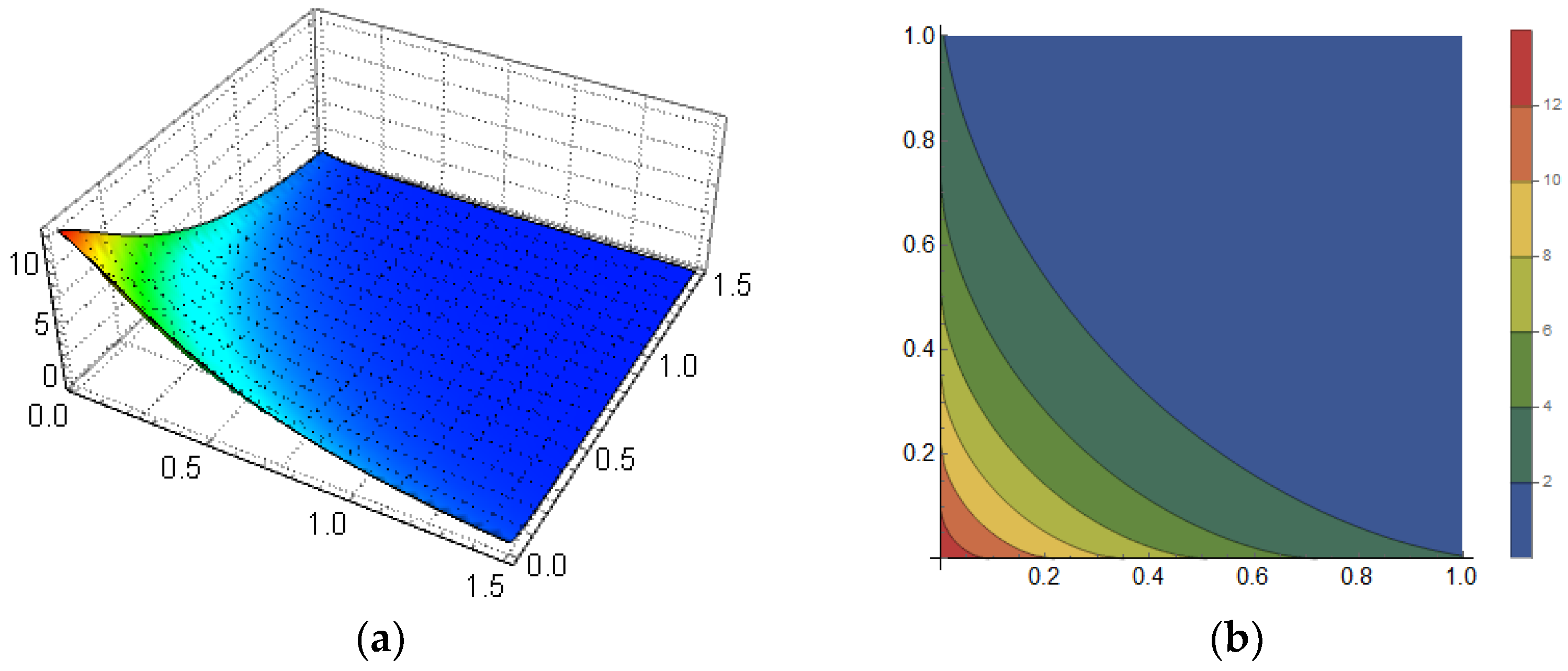
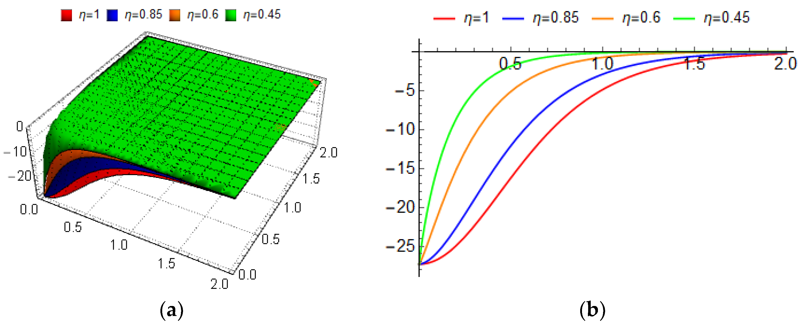
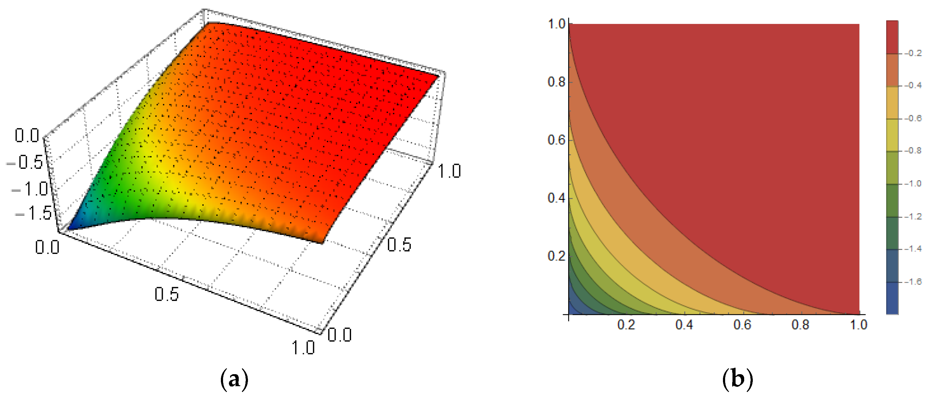
3.1. Nondifferentiable Solution-Type I

To construct the first nondifferentiable solution, ${\mathsf{\Phi }}_1$, for the local fractional ordinary differential Equation (28), we suppose it in the following form

$${\mathsf{\Phi }}_1\left({\chi }^{\eta }\right)={\mathsf{\Pi }}_1{\sec \mathrm{h}}_{\eta }^2\left({\mathsf{\Pi }}_2{\chi }^{\eta }\right)=\frac{4{\mathsf{\Pi }}_1}{{\left({ℰ}_{\eta }\left({\mathsf{\Pi }}_2{\chi }^{\eta }\right)+{ℰ}_{\eta }\left(-{\mathsf{\Pi }}_2{\chi }^{\eta }\right)\right)}^2}$$

(29)

where ${\mathsf{\Pi }}_1$ and ${\mathsf{\Pi }}_2$ are nonzero constants to be determined.

The LFD of ${\mathsf{\Phi }}_1\left({\chi }^{\eta }\right)$, with aid of Theorem 1 and Remark 1, can be found as

$${\left(\frac{d^{\eta }{\mathsf{\Phi }}_1}{d{\chi }^{\eta }}\right)}^2\left(=,4,{\mathsf{\Pi }}_1,\frac{d^{\eta }}{d{\chi }^{\eta }},\left(\frac{1}{{\left({\mathcal{E}}_{\eta },\left({\mathsf{\Pi }}_2,{\chi }^{\eta }\right),+,{\mathcal{E}}_{\eta },\left(-{\mathsf{\Pi }}_2{\chi }^{\eta }\right)\right)}^2}\right)\right)2$$

(30)

$$=4{\mathsf{\Pi }}_1^2{\mathsf{\Pi }}_2^2{\left(\frac{4\left({\mathcal{E}}_{\eta }\left({\mathsf{\Pi }}_2{\chi }^{\eta }\right)-{\mathcal{E}}_{\eta }\left(-{\mathsf{\Pi }}_2{\chi }^{\eta }\right)\right)}{{\left({\mathcal{E}}_{\eta }\left({\mathsf{\Pi }}_2{\chi }^{\eta }\right)+{\mathcal{E}}_{\eta }\left(-{\mathsf{\Pi }}_2{\chi }^{\eta }\right)\right)}^3}\right)}^2$$

$$=4{\mathsf{\Pi }}_1^2{\mathsf{\Pi }}_2^2\left(\frac{16{\left({\mathcal{E}}_{\eta }\left({\mathsf{\Pi }}_2{\chi }^{\eta }\right)-{\mathcal{E}}_{\eta }\left(-{\mathsf{\Pi }}_2{\chi }^{\eta }\right)\right)}^2}{{\left({\mathcal{E}}_{\eta }\left({\mathsf{\Pi }}_2{\chi }^{\eta }\right)+{\mathcal{E}}_{\eta }\left(-{\mathsf{\Pi }}_2{\chi }^{\eta }\right)\right)}^6}\right)$$

On the other hand, we obtain

$$4{\mathsf{\Pi }}_2^2{\mathsf{\Phi }}_1^2\left({\chi }^{\eta }\right)-\frac{4{\mathsf{\Pi }}_2^2}{{\mathsf{\Pi }}_1}{\mathsf{\Phi }}_1^3\left({\chi }^{\eta }\right)$$

(31)

$$=4{\mathsf{\Pi }}_2^2{\left(\frac{4{\mathsf{\Pi }}_1}{{\left({\mathcal{E}}_{\eta }\left({\mathsf{\Pi }}_2{\chi }^{\eta }\right)+{\mathcal{E}}_{\eta }\left(-{\mathsf{\Pi }}_2{\chi }^{\eta }\right)\right)}^2}\right)}^2$$

$$-\frac{4{\mathsf{\Pi }}_2^2}{{\mathsf{\Pi }}_1}{\left(\frac{4{\mathsf{\Pi }}_1}{{\left({\mathcal{E}}_{\eta }\left({\mathsf{\Pi }}_2{\chi }^{\eta }\right)+{\mathcal{E}}_{\eta }\left(-{\mathsf{\Pi }}_2{\chi }^{\eta }\right)\right)}^2}\right)}^3$$

$$=4{\mathsf{\Pi }}_1^2{\mathsf{\Pi }}_2^2\left(\frac{16}{{\left({\mathcal{E}}_{\eta }\left({\mathsf{\Pi }}_2{\chi }^{\eta }\right)+{\mathcal{E}}_{\eta }\left(-{\mathsf{\Pi }}_2{\chi }^{\eta }\right)\right)}^4}-\frac{64}{{\left({\mathcal{E}}_{\eta }\left({\mathsf{\Pi }}_2{\chi }^{\eta }\right)+{\mathcal{E}}_{\eta }\left(-{\mathsf{\Pi }}_2{\chi }^{\eta }\right)\right)}^6}\right)$$

$$=4{\mathsf{\Pi }}_1^2{\mathsf{\Pi }}_2^2\left(\frac{16\left({\left({\mathcal{E}}_{\eta }\left({\Pi }_2{\chi }^{\eta }\right)+{\mathcal{E}}_{\eta }\left(-{\Pi }_2{\chi }^{\eta }\right)\right)}^2-4\right)}{{\left({\mathcal{E}}_{\eta }\left({\Pi }_2{\chi }^{\eta }\right)+{\mathcal{E}}_{\eta }\left(-{\Pi }_2{\chi }^{\eta }\right)\right)}^6}\right)$$

Based on the analysis given in (30) and (31), we ensure that ${\mathsf{\Phi }}_1\left(\chi \right)$ satisfies the following relation

$${\left(\frac{d^{\eta }{\mathsf{\Phi }}_1}{d{\chi }^{\eta }}\right)}^2=4{\mathsf{\Pi }}_2^2{\mathsf{\Phi }}_1^2\left({\chi }^{\eta }\right)-\frac{4{\mathsf{\Pi }}_2^2}{{\mathsf{\Pi }}_1}{\mathsf{\Phi }}_1^3\left({\chi }^{\eta }\right)$$

(32)

By comparing the Equation (28) and the obtained relation (32), the constants ${\mathsf{\Pi }}_1$ and ${\mathsf{\Pi }}_2$ read as

$${\mathsf{\Pi }}_1=\frac{-3\left({\alpha }^{\eta }{\beta }^{\eta }+a_3{\beta }^{2\eta }+a_4{\gamma }^{2\eta }+a_5{\delta }^{2\eta }+a_6{\beta }^{\eta }{\gamma }^{\eta }+a_7{\beta }^{\eta }{\delta }^{\eta }+a_8{\gamma }^{\eta }{\delta }^{\eta }\right)}{a_1{\beta }^{2\eta }}$$

(33)

$${\mathsf{\Pi }}_2^{\pm }=\pm \sqrt{\frac{-\left({\alpha }^{\eta }{\beta }^{\eta }+a_3{\beta }^{2\eta }+a_4{\gamma }^{2\eta }+a_5{\delta }^{2\eta }+a_6{\beta }^{\eta }{\gamma }^{\eta }+a_7{\beta }^{\eta }{\delta }^{\eta }+a_8{\gamma }^{\eta }{\delta }^{\eta }\right)}{4a_2{\beta }^{4\eta }}}$$

(34)

Inserting (33) and (34) into (28), we get the following solution for the local fractional ordinary differential Equation (28):

$${\mathsf{\Phi }}_1^{\pm }\left({\chi }^{\eta }\right)=\left(\frac{-3\left({\alpha }^{\eta }{\beta }^{\eta }+a_3{\beta }^{2\eta }+a_4{\gamma }^{2\eta }+a_5{\delta }^{2\eta }+a_6{\beta }^{\eta }{\gamma }^{\eta }+a_7{\beta }^{\eta }{\delta }^{\eta }+a_8{\gamma }^{\eta }{\delta }^{\eta }\right)}{a_1{\beta }^{2\eta }}\right)$$

(35)

$$\times {\sec \mathrm{h}}_{\eta }^2\left(\left(\pm \sqrt{\frac{-\left({\alpha }^{\eta }{\beta }^{\eta }+a_3{\beta }^{2\eta }+a_4{\gamma }^{2\eta }+a_5{\delta }^{2\eta }+a_6{\beta }^{\eta }{\gamma }^{\eta }+a_7{\beta }^{\eta }{\delta }^{\eta }+a_8{\gamma }^{\eta }{\delta }^{\eta }\right)}{4a_2{\beta }^{4\eta }}}\right){\chi }^{\eta }\right)$$

Consequently, the traveling-wave solution for the LFKPE (1) can be written as

$$\begin{gathered} {\varphi }_1^{\pm }\left(t,x,y,z\right)=\left(\frac{-3\left({\alpha }^{\eta }{\beta }^{\eta }+a_3{\beta }^{2\eta }+a_4{\gamma }^{2\eta }+a_5{\delta }^{2\eta }+a_6{\beta }^{\eta }{\gamma }^{\eta }+a_7{\beta }^{\eta }{\delta }^{\eta }+a_8{\gamma }^{\eta }{\delta }^{\eta }\right)}{a_1{\beta }^{2\eta }}\right) \\ \times {\mathrm{sech}}_{\eta }^2\left(\left(\pm \sqrt{\frac{-\left({\alpha }^{\eta }{\beta }^{\eta }+a_3{\beta }^{2\eta }+a_4{\gamma }^{2\eta }+a_5{\delta }^{2\eta }+a_6{\beta }^{\eta }{\gamma }^{\eta }+a_7{\beta }^{\eta }{\delta }^{\eta }+a_8{\gamma }^{\eta }{\delta }^{\eta }\right)}{4a_2{\beta }^{4\eta }}}\right)\left({\alpha }^{\eta }{t}^{\eta }+{\beta }^{\eta }{x}^{\eta }+{\gamma }^{\eta }{y}^{\eta }+{\delta }^{\eta }{z}^{\eta }\right)\right) \end{gathered}$$

(36)

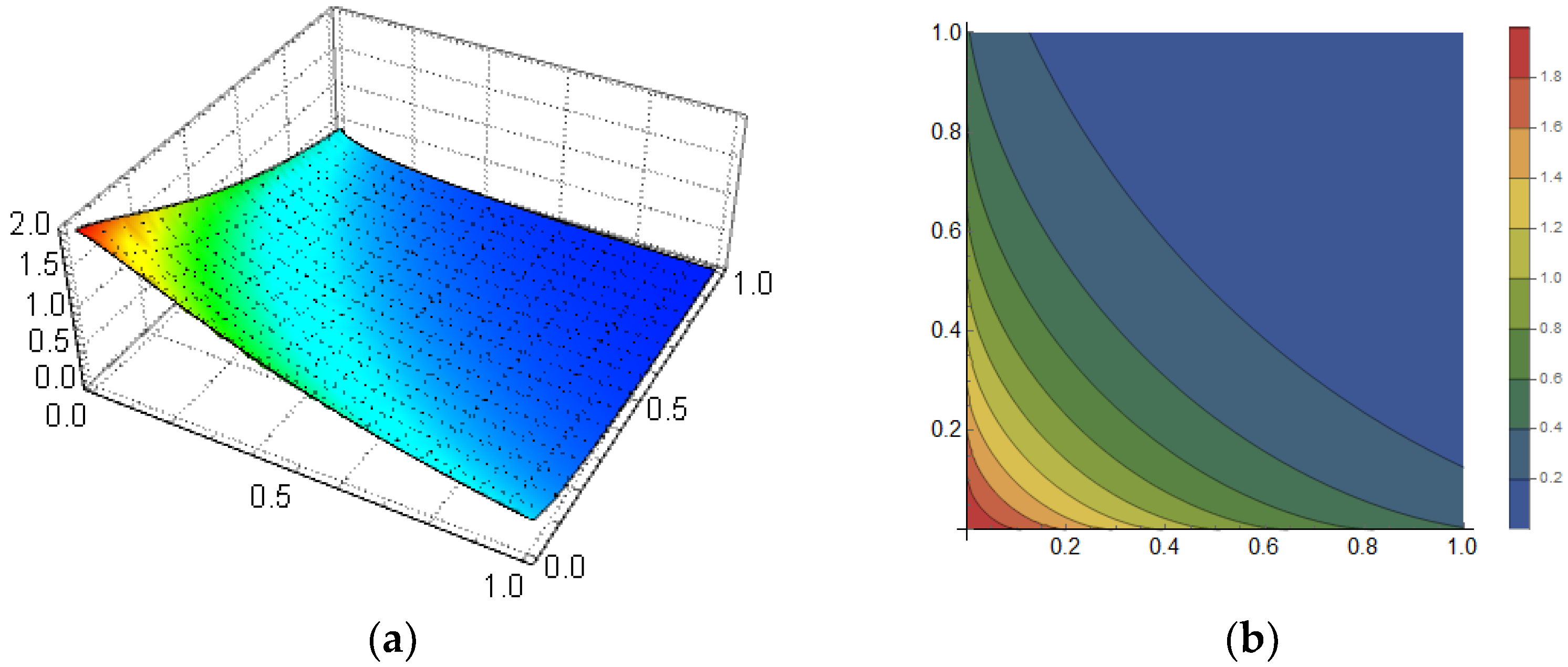
3.2. Nondifferentiable Solution-Type II

To construct another traveling-wave solution for LFKPE (1), we suppose the nondifferentiable solution for the local fractional ordinary differential equation (LFODE) (28) can be taken in the following form

$${\mathsf{\Phi }}_2\left({\chi }^{\eta }\right)={\mathsf{\Pi }}_3{\csc \mathrm{h}}_{\eta }^2\left({\mathsf{\Pi }}_4{\chi }^{\eta }\right)=\frac{4{\mathsf{\Pi }}_3}{{\left({ℰ}_{\eta }\left({\mathsf{\Pi }}_4{\chi }^{\eta }\right)-{ℰ}_{\eta }\left(-{\mathsf{\Pi }}_4{\chi }^{\eta }\right)\right)}^2},$$

(37)

where ${\mathsf{\Pi }}_3$ and ${\mathsf{\Pi }}_4$ are nonzero constants to be determined. Use the properties of the LFD with the similar technique in the previous section to ensure that ${\mathsf{\Phi }}_2\left({\chi }^{\eta }\right)$ satisfies the following relation

$${\left(\frac{d^{\eta }{\mathsf{\Phi }}_2}{d{\chi }^{\eta }}\right)}^2=-4{\mathsf{\Pi }}_2^2{\mathsf{\Phi }}_2^2\left({\chi }^{\eta }\right)-\frac{4{\mathsf{\Pi }}_2^2}{{\mathsf{\Pi }}_1}{\mathsf{\Phi }}_2^3\left({\chi }^{\eta }\right).$$

(38)

Therefore, comparing the coefficients of the local fractional ordinary differential equation (LFODE) (28) with the constructed relation (38), we deduce the following values for the constants ${\mathsf{\Pi }}_3$ and ${\mathsf{\Pi }}_4$

$${\mathsf{\Pi }}_3=\frac{3\left({\alpha }^{\eta }{\beta }^{\eta }+a_3{\beta }^{2\eta }+a_4{\gamma }^{2\eta }+a_5{\delta }^{2\eta }+a_6{\beta }^{\eta }{\gamma }^{\eta }+a_7{\beta }^{\eta }{\delta }^{\eta }+a_8{\gamma }^{\eta }{\delta }^{\eta }\right)}{a_1{\beta }^{2\eta }},$$

(39)

$${\mathsf{\Pi }}_4^{\pm }=\pm \sqrt{\frac{\left({\alpha }^{\eta }{\beta }^{\eta }+a_3{\beta }^{2\eta }+a_4{\gamma }^{2\eta }+a_5{\delta }^{2\eta }+a_6{\beta }^{\eta }{\gamma }^{\eta }+a_7{\beta }^{\eta }{\delta }^{\eta }+a_8{\gamma }^{\eta }{\delta }^{\eta }\right)}{4a_2{\beta }^{4\eta }}}.$$

(40)

Accordingly, the second traveling-wave solution for the LFKPE (1) can be written as

$$\begin{gathered} {\varphi }_2^{\pm }\left(t,x,y,z\right)=\left(\frac{3\left({\alpha }^{\eta }{\beta }^{\eta }+a_3{\beta }^{2\eta }+a_4{\gamma }^{2\eta }+a_5{\delta }^{2\eta }+a_6{\beta }^{\eta }{\gamma }^{\eta }+a_7{\beta }^{\eta }{\delta }^{\eta }+a_8{\gamma }^{\eta }{\delta }^{\eta }\right)}{a_1{\beta }^{2\eta }}\right) \\ \times {\csc \mathrm{h}}_{\eta }^2\left(\left(\pm \sqrt{\frac{\left({\alpha }^{\eta }{\beta }^{\eta }+a_3{\beta }^{2\eta }+a_4{\gamma }^{2\eta }+a_5{\delta }^{2\eta }+a_6{\beta }^{\eta }{\gamma }^{\eta }+a_7{\beta }^{\eta }{\delta }^{\eta }+a_8{\gamma }^{\eta }{\delta }^{\eta }\right)}{4a_2{\beta }^{4\eta }}}\right)\left({\alpha }^{\eta }{t}^{\eta }+{\beta }^{\eta }{x}^{\eta }+{\gamma }^{\eta }{y}^{\eta }+{\delta }^{\eta }{z}^{\eta }\right)\right) \end{gathered}$$

(41)

The graphical representation of the inferred traveling-wave solution (36) for the LFKPE (1) is presented in the following figures. Figure 1 shows the 3D plot and the contour plot of ${\varphi }_1^{+}\left(t,x,0,0\right)$ at the fractional derivative order at selected the parameters. The effect of the local fractional derivative on the observed traveling-wave solution ${\varphi }_1^{-}\left(t,x,0,0\right)$ has been illustrated in Figure 2. In Figure 3, we show the contour plot of the obtained traveling-wave solution ${\varphi }_2^{+}\left(t,x,0,0\right)$ at some selected parameters, in which the derivative is considered in an integer and fractional sense. It is clear from Figure 2 and Figure 3 that the fractional derivative mainly affects the intensity of the convexity in the form of the inferred solution. Figure 4 presents the 2D plot of the constructed exact solution ${\varphi }_2^{+}\left(t,x,0,0\right)$ at the diverse selected parameters to present a comparison in behavior of the traveling-wave solutions at different values for the spatial variable $x$ and at two opposite values for the dispersion parameters $a_1$

4. Nondifferentiable Solutions for LFKP-MEWE

In this section, we seek to explore nondifferentiable traveling-wave solutions for the LFKP-MEWE (2). To this purpose, we consider a nondifferentiable traveling-wave transformation in the form:

$$\varphi \left(t,x,y\right)=\mathsf{\Phi }\left({\chi }^{\eta }\right), {\chi }^{\eta }={\alpha }^{\eta }{t}^{\eta }+{\beta }^{\eta }{x}^{\eta }+{\gamma }^{\eta }{y}^{\eta },$$

(42)

where ${\alpha }^{\eta }, {\beta }^{\eta }$, and ${\gamma }^{\eta }$ are nonzero constants.

Substitute this transformation into the LFKP-MEWE (2), with the aid of the properties of the LFD, and simplify the resultant to infer the following local fractional ordinary differential equation:

$$\left({\alpha }^{\eta }{\beta }^{\eta }+{\gamma }^{2\eta }{a}_3\right)\frac{d^{2\eta }\mathsf{\Phi }}{d{\chi }^{2\eta }}+3{\beta }^{2\eta }{a}_1\left({\mathsf{\Phi }}^2\frac{d^{2\eta }\mathsf{\Phi }}{d{\chi }^{2\eta }}+2\mathsf{\Phi }{\left(\frac{d^{\eta }\mathsf{\Phi }}{d{\chi }^{\eta }}\right)}^2\right)+{\alpha }^{\eta }{\beta }^{3\eta }{a}_2\frac{d^{4\eta }\mathsf{\Phi }}{d{\chi }^{4\eta }}=0.$$

(43)

Use the chain rule to rewrite Equation (43) as follows:

$$\frac{d^{2\eta }}{d{\chi }^{2\eta }}\left(\left({\alpha }^{\eta }{\beta }^{\eta }+{\gamma }^{2\eta }{a}_3\right)\mathsf{\Phi }+{\beta }^{2\eta }{a}_1{\mathsf{\Phi }}^3+{\alpha }^{\eta }{\beta }^{3\eta }{a}_2\frac{d^{2\eta }\mathsf{\Phi }}{d{\chi }^{2\eta }}\right)=0$$

(44)

Utilize the LFI to both sides of the local fractional ordinary differential Equation (44) twice with zero integrating constants to obtain

$$\left({\alpha }^{\eta }{\beta }^{\eta }+{\gamma }^{2\eta }{a}_3\right)\mathsf{\Phi }+{\beta }^{2\eta }{a}_1{\mathsf{\Phi }}^3+{\alpha }^{\eta }{\beta }^{3\eta }{a}_2\frac{d^{2\eta }\mathsf{\Phi }}{d{\chi }^{2\eta }}=0$$

(45)

Multiplying the local fractional ordinary differential Equation (44) by the differential operator $\frac{d^{\eta }\mathsf{\Phi }}{d{\chi }^{\eta }}$ and, then, using the chain rule leads to the following equation

$$\frac{d^{\eta }}{d{\chi }^{\eta }}\left(\frac{\left({\alpha }^{\eta }{\beta }^{\eta }+{\gamma }^{2\eta }{a}_3\right)}{2}{\mathsf{\Phi }}^2+\frac{{\beta }^{2\eta }{a}_1}{4}{\mathsf{\Phi }}^4+\frac{{\alpha }^{\eta }{\beta }^{3\eta }{a}_2}{2}{\left(\frac{d^{\eta }\mathsf{\Phi }}{d{\chi }^{\eta }}\right)}^2\right)=0.$$

(46)

Apply the LFI to (46) and consider the integrating constant to be zero. Thus, the corresponding local fractional ordinary differential Equation (46) can be written as

$$\frac{\left({\alpha }^{\eta }{\beta }^{\eta }+{\gamma }^{2\eta }{a}_3\right)}{2}{\mathsf{\Phi }}^2+\frac{{\beta }^{2\eta }{a}_1}{4}{\mathsf{\Phi }}^4+\frac{{\alpha }^{\eta }{\beta }^{3\eta }{a}_2}{2}{\left(\frac{d^{\eta }\mathsf{\Phi }}{d{\chi }^{\eta }}\right)}^2=0.$$

(47)

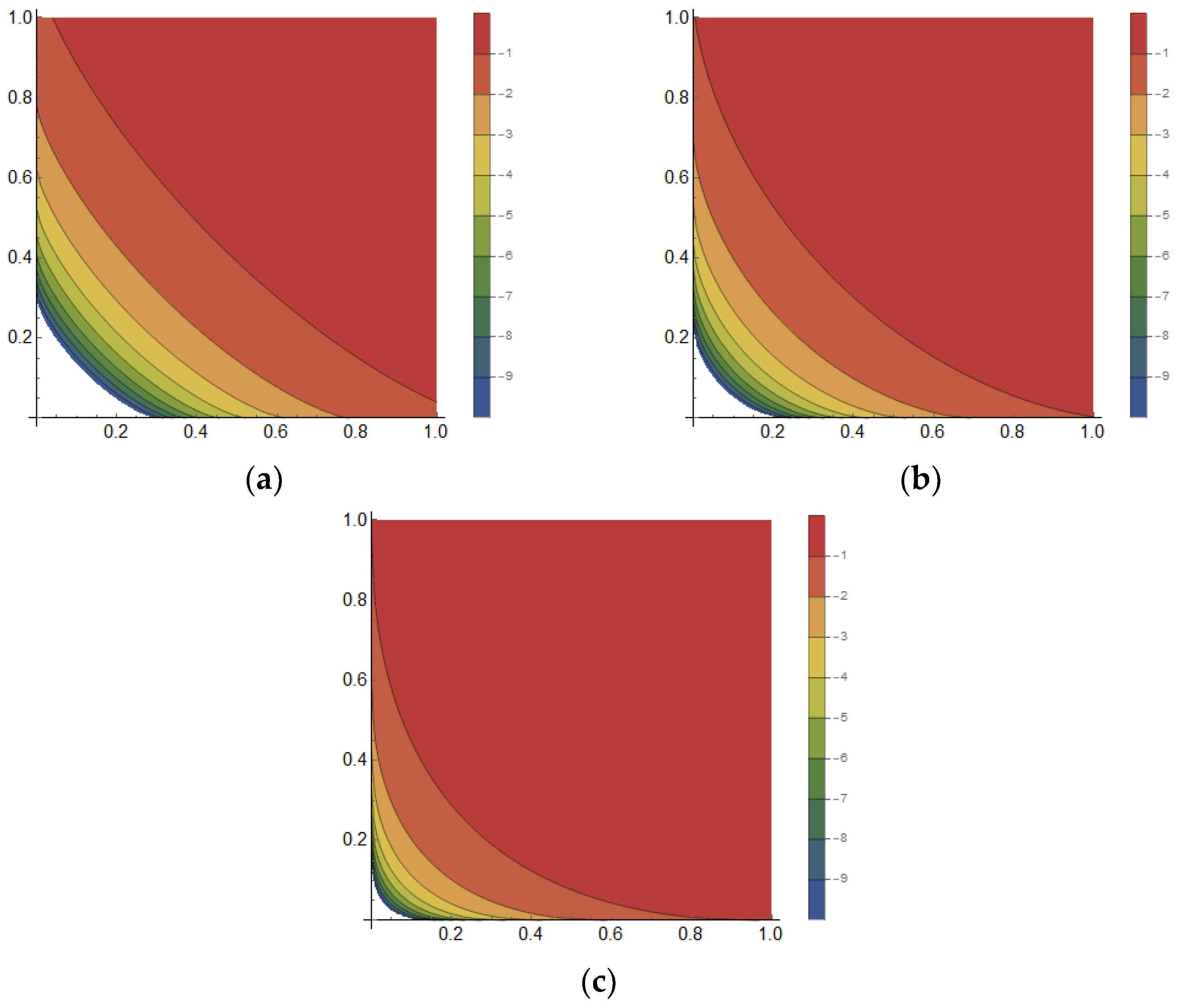
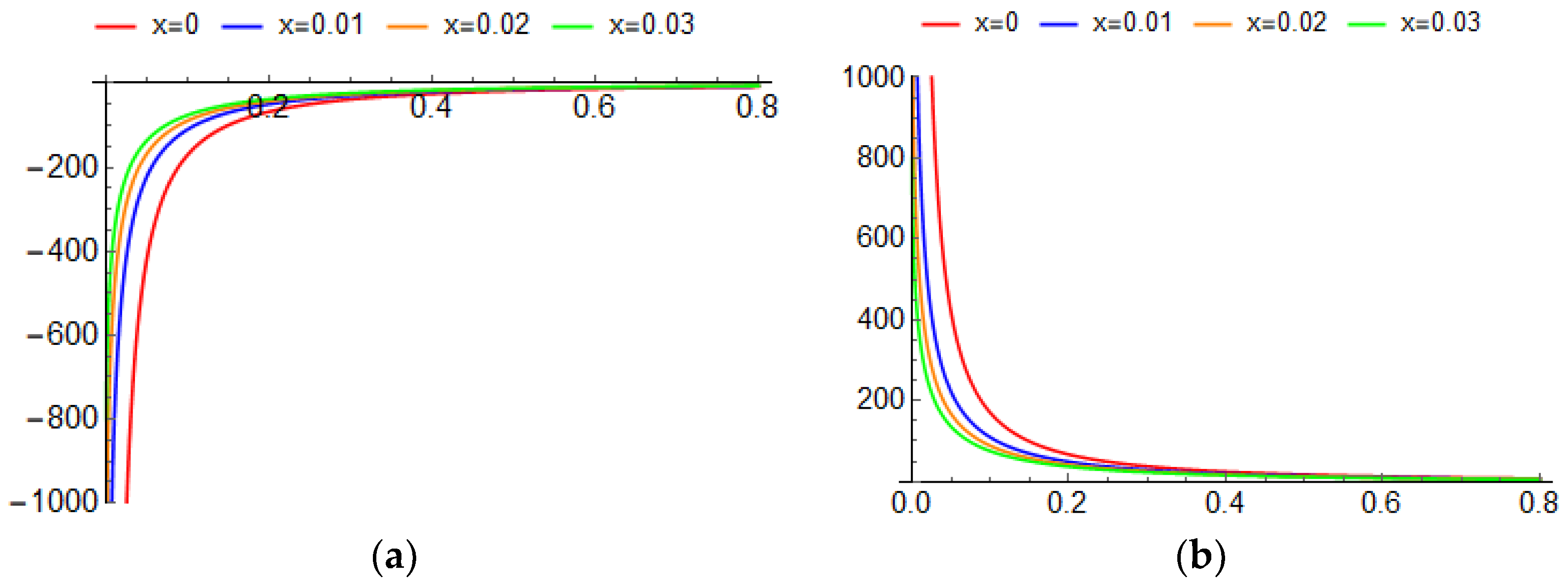
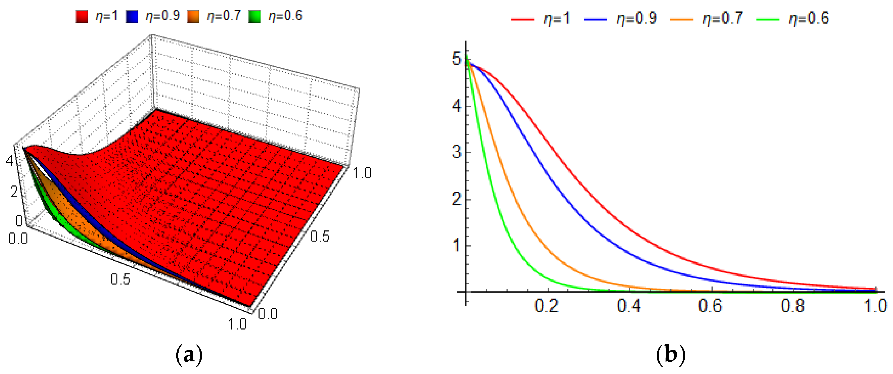
4.1. Nondifferentiable Exact Solution-Type I

We construct the first nondifferentiable traveling-wave solution for the local fractional ordinary differential Equation (45) in the form

$${\mathsf{\Phi }}_1\left({\chi }^{\eta }\right)={\mathsf{\Pi }}_1{\sec \mathrm{h}}_{\eta }\left({\mathsf{\Pi }}_2{\chi }^{\eta }\right)=\frac{2{\mathsf{\Pi }}_1}{{ℰ}_{\eta }\left({\mathsf{\Pi }}_2{\chi }^{\eta }\right)+{ℰ}_{\eta }\left(-{\mathsf{\Pi }}_2{\chi }^{\eta }\right)},$$

(48)

where ${\mathsf{\Pi }}_1$ and ${\mathsf{\Pi }}_2$ are constants to be determined. The LFD of ${\mathsf{\Phi }}_1\left({\chi }^{\eta }\right)$ can be observed as follows:

$${\left(\frac{d^{\eta }{\mathsf{\Phi }}_1}{d{\chi }^{\eta }}\right)}^2={\mathsf{\Pi }}_1^2{\left(\frac{d^{\eta }}{d{\chi }^{\eta }}\left(\frac{2}{{\mathcal{E}}_{\eta }\left({\mathsf{\Pi }}_2{\chi }^{\eta }\right)+{\mathcal{E}}_{\eta }\left(-{\mathsf{\Pi }}_2{\chi }^{\eta }\right)}\right)\right)}^2$$

(49)

$$={\mathsf{\Pi }}_1^2{\mathsf{\Pi }}_2^2{\left(\frac{2\left({\mathcal{E}}_{\eta }\left({\mathsf{\Pi }}_2{\chi }^{\eta }\right)-{\mathcal{E}}_{\eta }\left(-{\mathsf{\Pi }}_2{\chi }^{\eta }\right)\right)}{{\left({\mathcal{E}}_{\eta }\left({\mathsf{\Pi }}_2{\chi }^{\eta }\right)+{\mathcal{E}}_{\eta }\left(-{\mathsf{\Pi }}_2{\chi }^{\eta }\right)\right)}^2}\right)}^2$$

$$=4{\mathsf{\Pi }}_1^2{\mathsf{\Pi }}_2^2\left(\frac{{\left({\mathcal{E}}_{\eta }\left({\mathsf{\Pi }}_2{\chi }^{\eta }\right)-{\mathcal{E}}_{\eta }\left(-{\mathsf{\Pi }}_2{\chi }^{\eta }\right)\right)}^2}{{\left({\mathcal{E}}_{\eta }\left({\mathsf{\Pi }}_2{\chi }^{\eta }\right)+{\mathcal{E}}_{\eta }\left(-{\mathsf{\Pi }}_2{\chi }^{\eta }\right)\right)}^4}\right)$$

$$=4{\mathsf{\Pi }}_1^2{\mathsf{\Pi }}_2^2\left(\frac{{\left({\mathcal{E}}_{\eta }\left({\mathsf{\Pi }}_2{\chi }^{\eta }\right)+{\mathcal{E}}_{\eta }\left(-{\mathsf{\Pi }}_2{\chi }^{\eta }\right)\right)}^2-4}{{\left({\mathcal{E}}_{\eta }\left({\mathsf{\Pi }}_2{\chi }^{\eta }\right)+{\mathcal{E}}_{\eta }\left(-{\mathsf{\Pi }}_2{\chi }^{\eta }\right)\right)}^4}\right)$$

$$={\mathsf{\Pi }}_1^2{\mathsf{\Pi }}_2^2\left(\frac{2^2}{{\left({\mathcal{E}}_{\eta }\left({\mathsf{\Pi }}_2{\chi }^{\eta }\right)+{\mathcal{E}}_{\eta }\left(-{\mathsf{\Pi }}_2{\chi }^{\eta }\right)\right)}^2}-\frac{2^4}{{\left({\mathcal{E}}_{\eta }\left({\mathsf{\Pi }}_2{\chi }^{\eta }\right)+{\mathcal{E}}_{\eta }\left(-{\mathsf{\Pi }}_2{\chi }^{\eta }\right)\right)}^4}\right)$$

$$={\mathsf{\Pi }}_1^2{\mathsf{\Pi }}_2^2\left({\sec \mathrm{h}}_{\eta }^2\left({\mathsf{\Pi }}_2{\chi }^{\eta }\right)-{\sec \mathrm{h}}_{\eta }^4\left({\mathsf{\Pi }}_2{\chi }^{\eta }\right)\right)={\mathsf{\Pi }}_2^2{\mathsf{\Phi }}_1^2-\frac{{\mathsf{\Pi }}_2^2}{{\mathsf{\Pi }}_1^2}{\mathsf{\Phi }}_1^4.$$

The analysis in (49) ensures the following relation for the assumption ${\mathsf{\Phi }}_1\left(\chi \right)$

$${\left(\frac{d^{\eta }{\mathsf{\Phi }}_1}{d{\chi }^{\eta }}\right)}^2={\mathsf{\Pi }}_2^2{\mathsf{\Phi }}_1^2-\frac{{\mathsf{\Pi }}_2^2}{{\mathsf{\Pi }}_1^2}{\mathsf{\Phi }}_1^4.$$

(50)

Compare the coefficients of the same terms in the LFODE (46) and the obtained relation (50) to deduce the following values for the constants ${\mathsf{\Pi }}_1$ and ${\mathsf{\Pi }}_2$:

$${\mathsf{\Pi }}_1^{\pm }=\pm \sqrt{\frac{2\left({\alpha }^{\eta }{\beta }^{\eta }+{\gamma }^{2\eta }{a}_3\right)}{{\beta }^{2\eta }{a}_1}}, {\mathsf{\Pi }}_2^{\pm }=\pm \sqrt{\frac{-\left({\alpha }^{\eta }{\beta }^{\eta }+{\gamma }^{2\eta }{a}_3\right)}{{\alpha }^{\eta }{\beta }^{3\eta }{a}_2}}.$$

(51)

Accordingly, the nondifferentiable traveling-wave solutions for the LFODE (47) can be given as

$${\mathsf{\Phi }}_1^{\pm }\left({\chi }^{\eta }\right)=\pm \sqrt{\frac{2\left({\alpha }^{\eta }{\beta }^{\eta }+{\gamma }^{2\eta }{a}_3\right)}{{\beta }^{2\eta }{a}_1}}{\sec \mathrm{h}}_{\eta }\left(\pm \sqrt{\frac{-\left({\alpha }^{\eta }{\beta }^{\eta }+{\gamma }^{2\eta }{a}_3\right)}{{\alpha }^{\eta }{\beta }^{3\eta }{a}_2}}{\chi }^{\eta }\right).$$

(52)

Consequently, the nondifferentiable exact traveling-wave solutions for the LFKP-MEWE (2) are observed to be

$${\varphi }_1^{\pm }\left(t,x,y\right)=\pm \sqrt{\frac{2\left({\alpha }^{\eta }{\beta }^{\eta }+{\gamma }^{2\eta }{a}_3\right)}{{\beta }^{2\eta }{a}_1}}{\sec \mathrm{h}}_{\eta }\left(\pm \sqrt{\frac{-\left({\alpha }^{\eta }{\beta }^{\eta }+{\gamma }^{2\eta }{a}_3\right)}{{\alpha }^{\eta }{\beta }^{3\eta }{a}_2}}\left({\alpha }^{\eta }{t}^{\eta }+{\beta }^{\eta }{x}^{\eta }+{\gamma }^{\eta }{y}^{\eta }\right)\right).$$

(53)

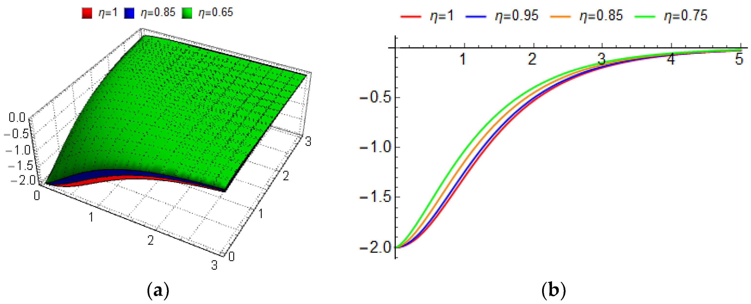
4.2. Nondifferentiable Exact Solution-Type II

We suppose that the nondifferentiable traveling-wave solution for the LFODE (47) can be written in the form

$${\mathsf{\Phi }}_2\left({\chi }^{\eta }\right)={\mathsf{\Pi }}_3{\sec }_{\eta }\left({\mathsf{\Pi }}_4{\chi }^{\eta }\right)=\frac{2{\mathsf{\Pi }}_3}{{ℰ}_{\eta }\left({\mathsf{\Pi }}_4{\left(i\chi \right)}^{\eta }\right)+{ℰ}_{\eta }\left(-{\mathsf{\Pi }}_4{\left(i\chi \right)}^{\eta }\right)}$$

(54)

where ${\mathsf{\Pi }}_3$ and ${\mathsf{\Pi }}_4$ are constants to be determined. Utilizing the same technique in (49) to infer the following relation of the assumption ${\mathsf{\Phi }}_2\left({\chi }^{\eta }\right)$

$${\left(\frac{d^{\eta }{\mathsf{\Phi }}_1}{d{\chi }^{\eta }}\right)}^2=-{\mathsf{\Pi }}_4^2{\mathsf{\Phi }}_1^2+\frac{{\mathsf{\Pi }}_4^2}{{\mathsf{\Pi }}_3^2}{\mathsf{\Phi }}_1^4$$

(55)

Compare the LFODE (47) and the obtained relation (55). Then, the values of the constants ${\mathsf{\Pi }}_3$ and ${\mathsf{\Pi }}_4$ fall to be

$${\mathsf{\Pi }}_3^{\pm }=\pm \sqrt{\frac{-2\left({\alpha }^{\eta }{\beta }^{\eta }+{\gamma }^{2\eta }{a}_3\right)}{{\beta }^{2\eta }{a}_1}}, {\mathsf{\Pi }}_4^{\pm }=\pm \sqrt{\frac{\left({\alpha }^{\eta }{\beta }^{\eta }+{\gamma }^{2\eta }{a}_3\right)}{{\alpha }^{\eta }{\beta }^{3\eta }{a}_2}}$$

(56)

Upon the observed result (56), the nondifferentiable traveling-wave solution for the LFODE (47) is given by

$${\mathsf{\Phi }}_2^{\pm }\left({\chi }^{\eta }\right)=\pm \sqrt{\frac{-2\left({\alpha }^{\eta }{\beta }^{\eta }+{\gamma }^{2\eta }{a}_3\right)}{{\beta }^{2\eta }{a}_1}}{\sec }_{\eta }\left(\pm \sqrt{\frac{\left({\alpha }^{\eta }{\beta }^{\eta }+{\gamma }^{2\eta }{a}_3\right)}{{\alpha }^{\eta }{\beta }^{3\eta }{a}_2}}{\chi }^{\eta }\right)$$

(57)

Therefore, we establish the nondifferentiable exact traveling-wave solution for the LFKP-MEWE (2) as follows

$${\varphi }_2^{\pm }\left(t,x,y\right)=\pm \sqrt{\frac{-2\left({\alpha }^{\eta }{\beta }^{\eta }+{\gamma }^{2\eta }{a}_3\right)}{{\beta }^{2\eta }{a}_1}}{\sec }_{\eta }\left(\pm \sqrt{\frac{\left({\alpha }^{\eta }{\beta }^{\eta }+{\gamma }^{2\eta }{a}_3\right)}{{\alpha }^{\eta }{\beta }^{3\eta }{a}_2}}\left({\alpha }^{\eta }{t}^{\eta }+{\beta }^{\eta }{x}^{\eta }+{\gamma }^{\eta }{y}^{\eta }\right)\right)$$

(58)

To understand the physical naturality of the established traveling-wave solution, we depict it in the following figures. Figure 5 represents the surface of the nondifferentiable traveling-wave solution ${\varphi }_1^{-}\left(t,x,0\right)$, at selected parameters, where the derivative is considered in a fractional sense. In Figure 6, we show the effect of the local fractional derivative on the inferred solutions ${\varphi }_1^{+}\left(t,x,0\right)$, at diverse fractional derivative orders, which illustrated that the intensity of the convexity of the constructed traveling-wave solutions has been affected with the change on the fractional derivative orders. Figure 7 represents the surface of the nondifferentiable traveling-wave solution ${\varphi }_2^{+}\left(t,x,0\right)$, at selected parameters, where the derivative is considered in a fractional sense. In Figure 8, we show the effect of the local fractional derivative on the inferred solutions and ${\varphi }_2^{-}\left(t,x,0\right)$, respectively, at diverse fractional derivative orders, which illustrated that the intensity of the convexity of the constructed traveling-wave solutions has been affected with the change on the fractional derivative orders.

5. Conclusions

In this article, the traveling-wave solutions of two significant nonlinear local fractional evolution equations, namely the fractional generalized (3 + 1)-dimensional Kadomtsev–Petviashvili equation and fractional Kadomtsev–Petviashvili-modified equal width equation, have been investigated under the local fractional derivative. The governing equations have been translated into local fractional ordinary differential equations by utilizing a traveling-wave transformation with a nondifferentiable type. The ansatz method is implemented to investigate nondifferentiable solutions for the proposed models based on the generalized functions defined on fractal sets. The obtained solutions are depicted in 2D, 3D, and contour plots at some selected parameters, where the derivative orders are considered in a fractional sense. The interesting obtained results show that the proposed technique is effective to explore traveling-wave solutions for diverse nonlinear partial differential equations. Fractal local derivatives will be of interest to explore fractal functions in future analysis such as the diffusion and convection models.

References

1. Yang, X.J.; Baleanu, D.; Srivastava, H.M. Local Fractional Integral Transforms and Their Applications, 1st ed.; Academic Press: Amsterdam, The Netherlands, 2016. [Google Scholar]
2. Atangana, A.; Baleanu, D. New fractional derivatives with non-local and non-singular kernel: Theory and application to heat transfer model. Therm. Sci. 2016, 20, 763–769. [Google Scholar] [CrossRef] [Green Version]
3. Al-Smadi, M.; Abu Arqub, O. Computational algorithm for solving fredholm time-fractional partial integrodifferential equations of dirichlet functions type with error estimates. Appl. Math. Comput. 2019, 342, 280–294. [Google Scholar] [CrossRef]
4. Al-Smadi, M.; Arqub, O.A.; Momani, S. Numerical computations of coupled fractional resonant Schrödinger equations arising in quantum mechanics under conformable fractional derivative sense. Phys. Scr. 2020, 95, 075218. [Google Scholar] [CrossRef]
5. Hasan, S.; Al-Smadi, M.; Freihet, A.; Momani, S. Two computational approaches for solving a fractional obstacle system in Hilbert space. Adv. Differ. Equ. 2019, 2019, 55. [Google Scholar] [CrossRef] [Green Version]
6. Freihet, A.; Hasan, S.; Al-Smadi, M.; Gaith, M.; Momani, S. Construction of fractional power series solutions to fractional stiff system using residual functions algorithm. Adv. Differ. Equ. 2019, 2019, 95. [Google Scholar] [CrossRef] [Green Version]
7. Baillie, R.T. Long memory processes and fractional integration in econometrics. J. Econ. 1996, 73, 5–59. [Google Scholar] [CrossRef]
8. Al-Smadi, M.; Arqub, O.A.; Hadid, S. An attractive analytical technique for coupled system of fractional partial differential equations in shallow water waves with conformable derivative. Commun. Theor. Phys. 2020, 72, 085001. [Google Scholar] [CrossRef]
9. Al-Smadi, M.; Arqub, O.A.; Zeidan, D. Fuzzy fractional differential equations under the Mittag-Leffler kernel differential operator of the ABC approach: Theorems and applications. Chaos Solitons Fractals 2021, 146, 110891. [Google Scholar] [CrossRef]
10. Al-Smadi, M.; Dutta, H.; Hasan, S.; Momani, S. On numerical approximation of Atangana-Baleanu-Caputo fractional integro-differential equations under uncertainty in Hilbert Space. Math. Model. Nat. Phenom. 2021, 16, 41. [Google Scholar] [CrossRef]
11. Günerhan, H.; Dutta, H.; Dokuyucu, M.A.; Adel, W. Analysis of a fractional HIV model with Caputo and constant proportional Caputo operators. Chaos Soliton Fractals 2020, 139, 110053. [Google Scholar] [CrossRef]
12. Al-Smadi, M.; Djeddi, N.; Momani, S.; Al-Omari, S.; Araci, S. An attractive numerical algorithm for solving nonlinear Caputo–Fabrizio fractional Abel differential equation in a Hilbert space. Adv. Differ. Equ. 2021, 2021, 271. [Google Scholar] [CrossRef]
13. Altawallbeh, Z.; Al-Smadi, M.; Komashynska, I.; Ateiwi, A. Numerical Solutions of Fractional Systems of Two-Point BVPs by Using the Iterative Reproducing Kernel Algorithm. Ukr. Math. J. 2018, 70, 687–701. [Google Scholar] [CrossRef]
14. Momani, S.; Freihat, A.; Al-Smadi, M. Analytical study of fractional-order multiple chaotic Fitzhugh-Nagumo neurons model using multistep generalized differential transform method. Abstr. Appl. Anal. 2014, 2014, 276279. [Google Scholar] [CrossRef] [PubMed] [Green Version]
15. Al-Smadi, M.; Freihat, A.; Arqub, O.A.; Shawagfeh, N. A novel multistep generalized differential transform method for solving fractional-order Lü chaotic and hyperchaotic systems. J. Comput. Anal. Appl. 2015, 19, 713–724. [Google Scholar]
16. Al-Smadi, M.; Arqub, O.A.; Hadid, S. Approximate solutions of nonlinear fractional Kundu-Eckhaus and coupled fractional massive Thirring equations emerging in quantum field theory using conformable residual power series method. Phys. Scr. 2020, 95, 105205. [Google Scholar] [CrossRef]
17. Alabedalhadi, M.; Al-Smadi, M.; Al-Omari, S.; Baleanu, D.; Momani, S. Structure of optical soliton solution for nonliear resonant space-time Schrödinger equation in conformable sense with full nonlinearity term. Phys. Scr. 2020, 95, 105215. [Google Scholar] [CrossRef]
18. Osman, M.S.; Korkmaz, A.; Rezazadeh, H.; Mirzazadeh, M.; Eslami, M.; Zhou, Q. The unified method for conformable time fractional Schro¨ dinger equation with perturbation terms. Chin. J. Phys. 2018, 56, 2500–2506. [Google Scholar] [CrossRef]
19. Islam, M.N.; Akbar, M.A. Closed form exact solutions to the higher dimensional fractional Schrodinger equation via the modified simple equation method. J. Appl. Math. Phys. 2018, 6, 90–102. [Google Scholar] [CrossRef] [Green Version]
20. Al-Smadi, M.; Arqub, O.A.; Gaith, M. Numerical simulation of telegraph and Cattaneo fractional-type models using adaptive reproducing kernel framework. Math. Methods Appl. Sci. 2021, 44, 8472–8489. [Google Scholar] [CrossRef]
21. Hasan, S.; Al-Smadi, M.; El-Ajou, A.; Momani, S.; Hadid, S.; Al-Zhour, Z. Numerical approach in the Hilbert space to solve a fuzzy Atangana-Baleanu fractional hybrid system. Chaos Solitons Fractals 2021, 143, 110506. [Google Scholar] [CrossRef]
22. Momani, S.; Djeddi, N.; Al-Smadi, M.; Al-Omari, S. Numerical investigation for Caputo-Fabrizio fractional Riccati and Bernoulli equations using iterative reproducing kernel method. Appl. Numer. Math. 2021, 170, 418–434. [Google Scholar] [CrossRef]
23. Yang, X.J.; Machado, J.T.; Baleanu, D.; Cattani, C. On exact traveling-wave solutions for local fractional Korteweg-de Vries equation. Chaos 2016, 26, 084312. [Google Scholar] [CrossRef] [PubMed]
24. Yang, X.J.; Machado, J.T.; Cattani, C.; Gao, F. On a fractal LC-electric circuit modeled by local fractional calculus. Commun. Nonlinear Sci. Numer. Simul. 2017, 47, 200–206. [Google Scholar] [CrossRef]
25. Yang, X.J.; Machado, J.A.; Nieto, J.J. A new family of the local fractional PDEs. Fundam. Inform. 2017, 151, 63–75. [Google Scholar] [CrossRef]
26. Babakhani, A.; Daftardar-Gejji, V. On calculus of local fractional derivatives. J. Math. Anal. Appl. 2002, 270, 66–79. [Google Scholar] [CrossRef] [Green Version]
27. Ahmad, J.; Mohyud-Din, S.T. Solving wave and diffusion equations on Cantor sets. Proc. Pak. Acad. Sci. 2015, 52, 81–87. [Google Scholar]
28. Kumar, D.; Singh, J.; Baleanu, D. A hybrid computational approach for Klein–Gordon equations on Cantor sets. Nonlinear Dyn. 2017, 87, 511–517. [Google Scholar] [CrossRef]
29. Singh, J.; Kumar, D.; Nieto, J.J. A reliable algorithm for a local fractional Tricomi equation arising in fractal transonic flow. Entropy 2016, 18, 206. [Google Scholar] [CrossRef] [Green Version]
30. Yang, X.J.; Machado, J.T.; Srivastava, H.M. A new numerical technique for solving the local fractional diffusion equation: Two-dimensional extended differential transform approach. Appl. Math. Comput. 2016, 274, 143–151. [Google Scholar] [CrossRef]
31. Yang, X.J.; Gao, F.; Srivastava, H.M. Exact travelling wave solutions for the local fractional two-dimensional Burgers-type equations. Comput. Math. Appl. 2017, 73, 203–210. [Google Scholar] [CrossRef]
32. Ghanbari, B. On novel nondifferentiable exact solutions to local fractional Gardner’s equation using an effective technique. Math. Methods Appl. Sci. 2021, 44, 4673–4685. [Google Scholar] [CrossRef]
33. Seadawy, A.R.; El-Rashidy, K. Dispersive solitary wave solutions of Kadomtsev-Petviashvili and modified Kadomtsev-Petviashvili dynamical equations in unmagnetized dust plasma. Results Phys. 2018, 8, 1216–1222. [Google Scholar] [CrossRef]
34. De Bouard, A.; Saut, J.C. Solitary waves of generalized Kadomtsev-Petviashvili equations. In Annales de l’Institut Henri Poincaré C, Analyse Non Linéaire; Elsevier Masson: Paris, France, 1997; Volume 14, pp. 211–236. [Google Scholar]
35. Groves, M.D.; Sun, S.M. Fully localised solitary-wave solutions of the three-dimensional gravity–capillary water-wave problem. Arch. Ration. Mech. Anal. 2008, 188, 1–91. [Google Scholar] [CrossRef] [Green Version]
36. Rao, J.; He, J.; Mihalache, D.; Cheng, Y. Dynamics and interaction scenarios of localized wave structures in the Kadomtsev–Petviashvili-based system. Appl. Math. Lett. 2019, 94, 166–173. [Google Scholar] [CrossRef]
37. Hao, X.; Liu, Y.; Li, Z.; Ma, W.X. Painlevé analysis, soliton solutions and lump-type solutions of the (3 + 1)-dimensional generalized KP equation. Comput. Math. Appl. 2019, 77, 724–730. [Google Scholar] [CrossRef]
38. Verma, P.; Kaur, L. Integrability, bilinearization and analytic study of new form of (3 + 1)-dimensional B-type Kadomstev–Petviashvili (BKP)-Boussinesq equation. Appl. Math. Comput. 2019, 346, 879–886. [Google Scholar] [CrossRef]
39. Yu, W.; Zhang, H.; Zhou, Q.; Biswas, A.; Alzahrani, A.K.; Liu, W. The mixed interaction of localized, breather, exploding and solitary wave for the (3 + 1)-dimensional Kadomtsev–Petviashvili equation in fluid dynamics. Nonlinear Dyn. 2020, 100, 1611–1619. [Google Scholar] [CrossRef]
40. Saha, A. Bifurcation of travelling wave solutions for the generalized KP-MEW equations. Commun. Nonlinear Sci. Numer. Simul. 2012, 17, 3539–3551. [Google Scholar] [CrossRef]
41. Gao, F.; Yang, X.J.; Ju, Y. Exact Traveling-Wave Solutions for One-Dimensional Modified Korteweg-De Vries Equation Defined on Cantor Sets. Fractal 2019, 27, 1940010. [Google Scholar] [CrossRef]
Figure 1. The profile of the traveling-wave solution ϕ 1 + ( t , x , 0 , 0 ) at: a 1 = 1 ,   a 2 = 1 ,   a 3 = 0.3 ,   a 4 = 1 ,   a 5 = 0.6 ,   a 6 = 0.1 ,   a 7 = 1 ,   a 8 = 1 ,   α = 0.1 ,   β = 0.1 ,   γ = 0.1 ,   δ = 0.1 : (a) 3D plot on t ,   x [ 0 ,   1.5 ] at η = ln ( 2 ) ln ( 3 ) ; (b) contour plot on t ,   x [ 0 ,   1 ] at η = ln ( 2 ) ln ( 3 ) .
Fractalfract 06 00210 g001
Figure 2. Effect of the local fractional derivative on the traveling-wave solution ϕ 1 ( t , x , 0 ) at: a 1 = 1 ,   a 2 = 1 ,   a 3 = 3 ,   a 4 = 1 ,   a 5 = 2 ,   a 6 = 0.1 ,   a 7 = 1 ,   a 8 = 1 ,   α = 0.1 ,   β = 0.1 ,   γ = 0.1 ,   δ = 0.1 on t , x [ 0 ,   2 ] where blue for η = 0.85 ; orange for η = 0.6 ; and green for η = 0.45 : (a) 3D plot of ϕ 1 ( t , x , 0 ) ; (b) 2D plot of ϕ 1 ( t , 0 , 0 ) .
Fractalfract 06 00210 g002
Figure 3. The profile of traveling-wave solution ϕ 2 + ( t , x , 0 , 0 ) at: a 1 = 6 ,   a 2 = 1 ,   a 3 = 1 ,   a 4 = 1 ,   a 5 = 1 ,   a 6 = 1 ,   a 7 = 1 ,   a 8 = 1 ,   α = 0.01 ,   β = 0.01 ,   γ = 0.001 ,   δ = 0.001 on x [ 0 , 1 ] and t [ 0 , 1 ] where: (a) η = 0.75 ; (b) η = ln ( 2 ) ln ( 3 ) ; (c) η = 0.5 .
Fractalfract 06 00210 g003
Figure 4. The profile of the traveling-wave solution ϕ 2 + ( t , 0 , 0 , 0 ) at: a 2 = 1 ,   a 3 = 1 ,   a 4 = 1 ,   a 5 = 0 ,   a 6 = 0 ,   a 7 = 0 ,   a 8 = 0 ,   α = 1 ,   β = 1 ,   γ = 1 ,   δ = 1 on t ∈ [0,0.8] where (a) 2D plot at a1 = −1; (b) 2D plot at a1 = 1, blue for 𝜂 = 0.01; orange for 𝜂 = 0.02; and green for 𝜂 = 0.03.
Fractalfract 06 00210 g004
Figure 5. The profile of ϕ 1 ( t , x , 0 ) at: a 1 = 2 ,   a 2 = 1 ,   a 3 = 2 ,   α = 1 ,   β = 1 ,   γ = 1 where: (a) the 3D plot at η = ln ( 2 ) ln ( 3 ) ; on x ∈ [0,1] and t ∈ [0,1]; (b) contour plot at η = ln ( 2 ) ln ( 3 ) ; on x ∈ [0,1] and t ∈ [0,1].
Fractalfract 06 00210 g005
Figure 6. Effect of the local fractional derivative on the traveling-wave solution ϕ 1 + ( t , x , 0 ) at a1 = 0.2, a2 = −0.1, a3 = 2, 𝛼 = 1.2, 𝛽 = 1.2, 𝛾 = 1 on t,x ∈ [0,1]: (a) 3D plot; (b) 2D plot.
Fractalfract 06 00210 g006
Figure 7. The profile of ϕ 2 + ( t , x , 0 ) at a1 = −1, a2 = −1, a3 = 1, 𝛼 = 1, 𝛽 = 1, 𝛾 = 1 where: (a) the 3D plot at η = ln ( 2 ) ln ( 3 ) on x ∈ [0,1] and t ∈ [0,1]; (b) the contour plot at η = ln ( 2 ) ln ( 3 ) on x ∈ [0,1] and on t ∈ [0,1].
Fractalfract 06 00210 g007
Figure 8. Effect of the local fractional derivative on the traveling-wave solution ϕ 2 ( t , x , 0 ) at a1 = −2, a2 = −4, a3 = 3, 𝛼 = 1, 𝛽 = 1, 𝛾 = 1 where: (a) the 3D plot at 𝜂 ∈ {1, 0.85, 0.65} on t,x ∈ [0,3]; (b) 2D plot at 𝜂 ∈ {1, 0.95, 0.85, 0.75} on t ∈ [0,5].
Fractalfract 06 00210 g008
Publisher’s Note: MDPI stays neutral with regard to jurisdictional claims in published maps and institutional affiliations.