
Dielectric Response Model for Transformer Insulation Using Frequency Domain Spectroscopy and Vector Fitting


1
Center for Research and Advanced Studies of Mexico (CINVESTAV), Campus Guadalajara, Zapopan 45019, Mexico
2
Advanced Design Center, Virginia Transformer Corporation, Chihuahua 31109, Mexico
*
Author to whom correspondence should be addressed.
Energies 2022, 15(7), 2655; https://doi.org/10.3390/en15072655
Submission received: 15 February 2022
/
Revised: 3 March 2022
/
Accepted: 7 March 2022
/
Published: 5 April 2022
(This article belongs to the Special Issue Compact Macromodeling: Components, Interconnects and Systems)
Abstract
:This paper proposes a rational approximation-based approach to find positive real parameters for the extended Debye model (EDM), aimed at condition assessment of insulation systems of power transformers. The EDM can model the slow and fast polarization phenomenon, including relaxation mechanisms with different relaxation times within a composite dielectric material. In the proposed approach, the complex permittivity of the transformer’s composite insulation is approximated via rational functions, as given by the vector fitting (VF) software tool, and the EDM parameters are identified from the obtained poles/residues. To guarantee positive real parameters, i.e., a physically realizable circuit, VF is internally modified to calculate the final residues of the rational approximation via a constrained linear least-squares problem without resorting to further post-processing algorithms, as in existing methods, hence without affecting fitting accuracy. The effectiveness of the parametrized EDM is demonstrated in two ways: (a) by reconstructing frequency domain spectroscopy (FDS) curves provided via measurements in new oil-immersed power transformers and (b) by the comparison of the calculated polarization current given by EDM versus real measurements in time domain. The achieved fitting accuracy in most of the cases is above 99 percent for the reconstructed FDS curves, while the polarization current waveform is reproduced with good agreement.
1. Introduction
Power transformers play a key role in power grid resiliency, as they constitute one of the grid’s most vulnerable components. Failure of a sole transformer can provoke at least momentary service interruption and can lead to significant collateral damage that might result in widespread cascading impacts with catastrophic consequences. To enhance the power grid’s resiliency, transformers must be operationally safe and reliable even at high operating temperatures due to overloads. Furthermore, they must endure electrical stresses due to transient overvoltages, lightning strikes, or switching maneuvers. Due to the abovementioned reasons, assessment of transformer condition and life management has become increasingly important. In this tenor, the transformer’s insulation system is a component that determines its life expectancy. In addition, it is its weakest component, generally representing the root cause of most catastrophic faults.
A variety of techniques have been used for monitoring, testing, and diagnosing power transformer insulation systems. A partial list is: insulation resistance (IR), polarization index (PI), partial discharges (PD), dissolved gas analysis (DGA), and general oil quality. More precise information on insulation health can also be obtained by using invasive techniques such as the degree of polymerization and furan analysis. Over the last few decades, attention has been directed toward modern techniques that measure changes in the dielectric properties of insulation. Those techniques are neither destructive nor invasive and are reliable for determining moisture content, aging of the paper insulation, and in general, for diagnosing power transformers [1]. The two leading modern techniques in time domain are the return (or recovery) voltage measurement (RVM) and the polarization and depolarization current (PDC) measurements, also known as dielectric spectroscopy (DS) in time domain. As for frequency domain techniques, the dielectric frequency domain spectroscopy (FDS) method measures the complex capacitance and the dissipation factor in a typical wideband from 1 mHz to 1 kHz [1], and the frequency response analysis (FRA) has been used as a diagnostic tool for assessing the mechanical integrity but has also been recently used for insulation assessment. FRA obtains the voltage transfer function of the transformer winding in a wideband from 20 Hz to 2 MHz [2].
The main challenge surrounding the aforementioned techniques is the interpretation of results. For a better interpretation, equivalent RC circuits are used for modeling the transformer insulation system. The frequency response of such RC circuits is used to analyze the transformer’s physical behavior and dielectric patterns. Moreover, the circuit parameters are strongly correlated to the transformer’s insulation condition, as they depend on its actual physical properties, i.e., degree of aging and water content.
In this paper, the extended Debye model is used to evaluate the dielectric characteristics of a power transformer. The values of the EDM parameter are identified via rational fitting of FDS curves using an internally modified version of VF that guarantees positive real RC parameters, i.e., a physically realizable circuit, maintaining the accuracy of the fitting. It is mentioned that existing methods use a post-processing algorithm to enforce parameters to be physically realizable, degrading at some extent fitting accuracy.
The paper is structured as follows. In Section 2, the paper describes a brief overview of the dielectric response concept. The classical and extended Debye models are described in Section 3, and parameter calculation methods are mentioned in Section 4. Section 5 explains the main concepts of the FDS. The basics of VF and the proposed modification are explained in Section 6 and Section 7. The validation of the proposed approach is presented in Section 8. The results are discussed in Section 9. Finally, the paper is concluded in Section 10.
2. Overview on Dielectric Response
The DS technique, either in time domain or frequency domain, permits the assessment of insulation system properties based on its dielectric response under the application of an electric field. The dielectric response is time dependent due to the polarization phenomenon in which the buildup of steady-state polarization requires a finite time to reach its maximum value. In the same way, when the electric field is suddenly removed, polarization will take a finite time to decay to zero. This phenomenon is called dielectric relaxation. There are essentially four types of polarization mechanisms: (i) electronic, (ii) ionic, (iii) dipole and (iv) interfacial. Mechanisms (i) and (ii) are extremely fast while (iii) and (iv) represent a slow phenomenon. Note that, in general, polarization is a time-varying phenomenon and implies a flow of charges constituting an electrical current. Therefore, the most important experimental procedure to determine polarization relies on the determination of the electric current resulting from the rate of change of polarization with respect to time.
Besides the conduction current due to the conductivity of the imperfect dielectrics, any insulation system will carry the so-called displacement current given by (1), where is the total charge moving within the dielectric material due to an external electric field. is the sum of the contribution of free space, which is instantaneous, and material medium polarization, which is time delayed and depends on the dielectric material properties [3].
The most dominant term of current arising in time-domain spectroscopy analysis is characterized by the response function of an insulation material due to its different polarization mechanisms. In the frequency domain, is related by the complex susceptibility via (2), where denotes the Fourier transform. provides information about the amplitude and phase of the polarization component, and it is a way to study the dielectric material properties by its response to alternating electric fields. Although each dielectric material has its own exclusive response, most of them show a typical response that can be characterized by , which allows for visualizing possible relaxation mechanisms.
3. Classical and Extended Debye Models
3.1. Classical Debye Model
The dielectric response of a physically realistic dielectric can be represented by the classical Debye model constructed with a simple RC branch and a further ideal parallel capacitor that represents the free space capacitance (or permittivity) at high frequencies where losses are not significant [3]. The equivalent circuit of the classical Debye model is presented in Figure 1a; its corresponding complex permittivity is given by
where
Relations (3) and (4) are known as the Debye equations. They are used to describe a dielectric system and to determine if the Debye relaxation is a possible mechanism. In Equations (3) and (4), and are the static and instantaneous (high frequency) relative permittivity, respectively, and is called the Debye dielectric relaxation time [4].
Debye’s model response is usually seen in simple dielectric liquids. A common dielectric response observed on many solid materials is based on power–law relaxation, also known as the Curie–von Schweidler model. According to this law, the current decays according to a power law:
where is the decay constant such that [1,5].
The circuit in Figure 1b, which corresponds to a parallel RC with a further capacitor , is suitable to represent any material that exhibits conduction. The expression for its complex permittivity is given by
where is the vacuum capacitance or geometrical capacitance and represents the capacitance that would be obtained on a capacitor if its dielectric material was replaced by a vacuum (free space) but kept the same geometry. In addition, in Equation (6), Note that in Equation (6), is independent of frequency and increases with decreasing frequency.
For a material that exhibits both relaxation and conduction behavior (see Figure 1c) has been replaced by a series RC arrange. Its complex permittivity is expressed now as
where and . This representation is known also as the Debye model for homogeneous lossy material.
3.2. Extdended Debye Model
For insulation systems made of mixtures of different dielectric materials, e.g., an insulating liquid with ionic conduction mixed with a lower conduction solid, as in an oil–paper insulation system, charge accumulation occurs at the interface due to the differences between their conductivities and dielectric constants . This phenomenon is known as interfacial polarization, or the Maxwell–Wagner effect. For such a mixture of different dielectric materials, polarization cannot be accurately modeled via the RC circuits of Figure 1, because in a composite insulation system, polarization is caused by different mechanisms with different relaxation time constants. Moreover, polarization is affected by moisture, aging, and temperature [3].
Although the Maxwell–Wagner model can be applied to a multilayer oil–paper insulation system [6], prevalent algorithms for frequency response analysis and assessment of oil–paper insulation systems are based on EDM or derived from an EDM approach.
The EDM (see Figure 2) is constructed by using a parallel arrangement of series-connected RC branches involving a resistor and a capacitor [7]. Each of these series connections provide a time constant given by that represents the different polarization processes randomly distributed within the insulation system. The conduction current is represented by the insulation resistance , and the geometrical capacitance of the insulation system is represented by a shunt capacitance .
The identification of the EDM circuit parameters is usually performed through dielectric response measurements either in time domain (PDC [7] and RVM [8,9] or in frequency domain (FDS [10,11]). This identification process leads to a multivariable nonlinear problem that is solved via mathematical techniques that involve numerical and iterative methods [8], exponential curve fitting [7], nonlinear programming [12] nonlinear least-squares optimization [11], and other combinations with heuristic optimization algorithms [10,13].
4. Calculation of EDM Parameters
Circuit parameters calculated from time-domain responses (RVM, PDC) exhibit an accurate reconstruction of recorded traces either individually, between reciprocal transformation RVM–PDC [7], or by transformations to frequency domain data (FDS) [14]. Hence, under ideal conditions, both time and frequency domain methods are comparable, although there are several disadvantages of the former when measurements are performed onsite. The most notable disadvantage is its vulnerability to electromagnetic interference when applying a DC voltage (PDC) that requires measurement of small currents [15].
Conversely, the main weakness of the FDS method is related to long measurement times at low frequencies. For example, it takes nearly 17 min to complete one sinusoidal cycle at 1.0 mHz. This low-frequency shortcoming is overcome with a recent approach that uses a multi-frequency test signal instead of a single frequency [15]. Therefore, the FDS method is now by far a better choice. Furthermore, the EDM identification directly using FDS instead of PDC or RVM leads to a better characterization of the insulation system, permitting a better interpretation and diagnosis of its condition [10].
Calculation of EDM parameters derived from FDS is a problem that has been addressed by other researchers; however, a few reports can be found in the specialized literature. In [10], the EDM parameters are identified using a syncretic algorithm that integrates a genetic algorithm and a Levenberg–Marquardt algorithm from FDS measurements performed in an oil-impregnated condenser bushing. In [12], the equivalent circuit model parameters for oil–paper insulation samples are obtained by a nonlinear optimization procedure from the dissipation factor curves; in this work, only one parallel branch is considered. In [13], the nonlinear problem of EDM parameters identification is solved by the nonlinear square method and bacterial foraging algorithm applied on scaled down transformer insulation models and with the data of FDS. In [11], a rational approximation of the FDS curve is derived via the VF method; however, a post-processing algorithm of least-squares optimization with constraint is required to enforce passivity; this technique is applied to a condenser transformer bushing as well.
In this paper, the complex capacitance curve, measured from a broadband FDS, is approximated by using rational functions via a modified version of VF. This modification permits the direct calculation of the EDM parameters, which guarantees the realizability of the circuit without any post-processing routine.
5. Frequency Domain Spectroscopy
FDS, also known as dielectric frequency response (DFR), is a dielectric analysis technique based on the same principle of the well-known capacitance and power factor/dissipation factor measured at one specific frequency value (close to line frequency 50/60 Hz). The DFR technique involves measurements over a wide frequency range, typically from an upper limit of 1 kHz down to a lower limit that ranges between 10 and 0.1 mHz. Traditional measurements at a single frequency are usually at 10 kV or at a voltage not greater than the rated voltage of the specimen under test, while DFR measurements are performed using low voltage (i.e., 140 V RMS) to avoid voltage-dependent effects at low frequencies, although higher voltages may be used in environments with high interference [16]. In a practical setup, DFR consists in both the application of a sinusoidal voltage across the terminals of the test object and the measurement of the amplitude and phase of the response current flowing through the insulation system.
When an electrical field is applied to an imperfect dielectric, the current can be defined based on its DC electrical conductivity and its dielectric displacement . To perform the dielectric response analysis in the frequency domain, this current can be expressed in terms of a current density as follows [3]:
For a better physical interpretation, in Equation (8), is expressed in terms of the complex permittivity where
The ratio can physically be better understood in terms of the ratio between a voltage and a current V, characterized by an impedance function or by an admittance . For insulation diagnostic and/or analysis, the complex capacitance model is more commonly used since it can describe either the insulation impedance or the insulation admittance.
The general definition of steady-state capacitance is applicable for , where instead of a constant voltage, an alternating voltage with frequency is employed. When this voltage is applied to a capacitive circuit, the resulting current can be expressed in terms of as
where
and
In practice, it is common to apply a voltage across the sample and to measure the current flow; hence, the impedance is easily calculated using Ohm’s law . The insulation impedance in the complex capacitance model is often described as a capacitance combined with a dissipation factor () [10] or with a power factor (), where
In some cases, it is more convenient to express in terms of the complex permittivity as
where the dielectric constant is given by the ratio of the complex permittivity to the permittivity of free space . The abovementioned reasoning establishes the basis to determine the effective permittivity of a dielectric system with a homogeneous material from the measurement of the impedance or the admittance.
6. Vector Fitting Basic Equations
For completeness of the paper, the VF basics are described in this Section. VF is a numerical algorithm to approximate frequency domain responses via rational functions [17]. Recently, VF has been extended to consider time-domain, z-domain, and scattering responses [18,19]. Note that only the basic VF algorithm is briefly described in the following, as it is sufficient for the identification of EDM.
The main objective of VF is to fit (approximate) a system transfer function H(s) via rational functions, as in Equation (15), where . The approximation in Equation (15) is represented as a summation of partial fractions composed of residues, , first-order poles, , and two optional terms, and .
The (unknown) terms and can be real or come in complex conjugate pairs, while and are real.
Since appears in the denominator of Equation (15), the identification problem becomes nonlinear. Hence, to overcome the nonlinearity problem, starting (known) poles are proposed in a first step. Usually, the proposed poles are assumed either linearly or logarithmically spaced along with the frequency band of the frequency response under interest [17].
As the second step, an unknown rational scaling function is introduced as
In such a way that the rational approximation of has the same known poles . In the third step, Equation (17) is formulated.
To calculate the unknown variables (, , and ), Equation (17) is evaluated at points of the frequency bandwidth, resulting in the system of linear Equation (18).
The fact that leads to the overdetermined linear system (18), which can be solved, for example, by using the MATLAB backslash operator “\”, which indicates matrix inversion computed in the least-squares sense. Once system (18) is solved for the unknown parameters, Equation (19) is readily obtained from
From Equation (19), the poles of correspond to the zeros of . Hence, the fourth step involves the calculation of the zeros of (poles of ), which can be readily achieved from the partial fraction representation, as in Equation (16). It is mentioned that VF can enforce stability by keeping all the poles in the left-half plane; that is, for any iteration that results in positives (unstable) poles, VF inverts the sign of their real parts.
Once the poles of are calculated, the residues and terms and in are computed in the fifth step by building and solving a linear overdetermined system , obtained from the evaluation of Equation (15).
The above-mentioned steps are implemented in an iterative fashion by using the new poles of as starting poles. The process ends when convergence is achieved.
7. Modified VF and FDS Algorithm for EDM Identification
Based on FDS measurements, the insulation system can be characterized via its complex capacitance, as defined in Equation (14), where can be obtained either by measurements or estimated by calculations. Moreover, the EDM in Figure 2, based on Equations (10) and (11), can be synthesized as the admittance given by Equation (20).
Comparing the EDM and Equation (20), each element of the model can easily be identified as
where is represented by the high-frequency capacitance [20].
The only constraint for Equation (20) to be physically realizable with an RC admittance is that residues must be real and positive, without affecting fitting accuracy. Positive real RC elements are also important to obtain realistic time constants of the polarization phenomenon. This realizability is addressed in this paper.
The DFR of dielectric materials and composite insulation systems are characterized by smooth curves (without resonance peaks), which can be fitted by low-order approximations using real poles in VF [17]. However, in some cases, the optimal (i.e., smallest approximation error) VF approximation leads to negative residues that make the function unphysically realizable. To address this problem, a second adjustment in the original formulation of VF is proposed in this paper as described next.
To enforce realizability, the linear system , formulated in the fifth step of the VF algorithm described in Section 6, is solved in the (internally) modified VF as the constrained linear least-squares problem:
where and are real vectors containing the lower and upper bounds, respectively.
The solution of (22) is performed in this paper by the trust–region–reflective algorithm, which is a subspace trust–region method based on the interior-reflective Newton method [21,22]. For such a solution, the MATLAB built-in function lsqlin is utilized. As an alternative, a nonnegative least-squares optimization can be used via the MATLAB built-in function lsqnonneg, which returns a vector that minimizes subject to . Although both functions work properly and converge to the same results for most of the cases, in this paper, the lsqlin function is utilized for the presented cases.
The following steps for the identification of the EDM realizable parameters are implemented in the MATLAB environment.
Step 1. The FDS data are exported from the measurement instrument and transformed into a complex capacitance form.
Step 2. The geometrical capacitance is calculated and used to generate frequency domain responses for the relative dielectric permittivity .
Step 3. The proposed modified version of VF is employed to find a rational approximation of using, as starting poles, real poles logarithmically spaced within the considered frequency wideband. The proposed algorithm chooses the order (number of branches) by sweeping from one to ten the order of approximation and keeping as a final approximation the order with the smallest rms error.
Step 4. Once the best fitting (lowest rms error) of is found, the parameter identification of EDM in an admittance form is performed, as given by Equations (20) and (21).
8. Validation
The dielectric frequency responses of six new power transformers between 25 and 115 kV class are obtained via an IDAX 300. The IDAX 300 is a MEGGER instrument that can measure the capacitance and dissipation factor (DF), or power factor (PF), of the insulation between power transformer windings at multiple frequencies, e.g., 1 mHz–1 kHz [23].
The parameters of the tested transformers are listed in Table 1. The dissipation factor percent (%DF), capacitance (C), moisture percent, and oil conductivity are the calculated values from the measurement instrument during FDS.
The DFR measurements are performed at the major barrier insulation between the high-voltage (HV) and low-voltage (LV) windings since this interwinding insulation contains most of the solid insulation in the overall transformer dielectric system.
The ungrounded specimen test configuration is used with the same setup and execution as the traditional power frequency capacitance and PF measurements [16]. The fitted and measured responses corresponding to DF and complex capacitance are presented in Figure 4 and Figure 5, respectively. The fitted curves are obtained by using the optimal quantity, i.e., with the lowest rms error, of RC-paralleled branches of the EDM, according to the modified VF, as described in Section 7.
The resultant EDM parameters for all transformers are listed in Table 2, where the time constant of each polarization branch can be calculated by . Note that all EDM-identified values are real and positive, which guarantee realizability. The accuracy of the fitting (AF) for the complex capacitances is calculated by using the normalized rms error expressed as a percentage, where 100% means a perfect fitting. Table 3 lists the AF for each transformer, the best fitting order and iteration in which is achieved, and the corresponding rms fitting errors.
As further validation of the effectiveness of the parametrized EDM, the calculated polarization current from FDS is compared with real measurements in the time domain, using a MIT1025 insulator resistance tester.
The theoretically expected current can be derived from the corresponding time domain of Equation (8) with constant , assumed as a step-like DC charging voltage divided by the radial distance between electrodes, as follows:
The first term in (23) represents the DC conductivity mechanism. The response function represents polarization processes that cannot respond instantaneously to the applied voltage and have a different time constant that is widely distributed. These terms can be measured to make a reliable diagnosis. The term involving the impulse function represents the fast polarization processes occurring in extremely short times; this cannot be recorded in practice since it involves a large amplitude, and it is avoided (discarded) during the measurement process. Thus, the practical measured polarization current is expressed as
where the magnitude is essentially a function of and the geometrical capacitance , may either be the vacuum capacitance or the high-frequency capacitance of insulation system at the time that the current measurement is started.
Conversely, the polarization current can be calculated from the EDM as
By comparing (24) and (25), it is easy to identify the DC resistance as .
Figure 6 presents the polarization currents for transformers #3, #5, and #6 only, given by time domain measurements and calculated from the parametrized EDM using FDS. The polarization current is measured for transformers #3 and #6 using a charging voltage of 500 and 1000 VDC for transformer #5. The charging time is 1200 s for all of them. Figure 6 shows good agreement between measurements and the identified EDM, thus validating the proposed approach.
9. Discussion
The identified parameters in Table 2 show the sensibility of the values to the condition and properties of the dielectric material comprising its insulation system. Each of the tested transformers have different moisture content and specific oil conductivity (oil quality), as shown in Table 1. In addition, these parameters have a strong dependence on the coil geometry as expected by Equation (21) since the coil height, diameters, and interwinding construction are customized and optimized based on its power, KV class, and specific performance required. However, it is not the intention of this paper to evaluate the correlation of the insulation properties with the obtained parameter values. The contribution of this work is intended to develop an effective algorithm that can be used to straightforwardly identify the EDM branch parameters whose values can be further correlated to the condition of a multilayer insulation system for diagnosis and decisions concerning life management, aging, or water content, among others. In future publications, the pole distribution in the complex plane is intended for achieving a better interpretation of the insulation system condition.
As for the tested transformers, there is not a general rule on the number of EDM RC branches, as seen in Table 2. In the proposed algorithm, the order (number of poles) is related to the number of branches in the EDM. Each branch represents a polarization process with a particular constant time; then, the number of branches will depend upon the nature of the tested transformer and its condition. Usually, six to ten branches are enough to achieve accurate approximations [10]. The results in this paper agree with such numbers, noting that seven to ten branches are enough to achieve an accuracy above 99.7% for and and above 97.6% for
Positive realness of the RC elements is guaranteed via the proposed approach. This permits (a) to calculate realistic time constants involved in the polarization process and (b) to accurately reproduce polarization currents avoiding unstable simulation.
The proposed algorithm compares the polarization current from the EDM-obtained parameters and from real FDS measurements. Figure 6 shows a fairly good agreement between the calculated and measured polarization current. The deviation seen in the first seconds (i.e., < 100 s) can be explained by referring to Equations (24) and (25) where the term which is of extremely short duration and high magnitude, is not recorded as already explained before. In addition, the accuracy of the first part of the polarization current during data acquisition, 0.1 to 1 s after switching, requires additional special equipment and other complex circuits. The data acquisition for the polarization current in this paper was performed with a Megger MIT1025 Insulation Resistance Tester [24] which does not have the accuracy of a sophisticated polarization current tester. The polarization current was recorded during the dielectric charge and discharge test. Although the current related to the response function is correctly recorded and represents the rest of the polarization processes that cannot respond instantaneously to the applied voltage, this polarization current arises in a delayed way to the applied voltage. This part characterizes the most important property of the dielectric systems. Then, the effort to increase the accuracy of the first part of the polarization current with aforesaid complexity in an instrument is not required [25].
10. Conclusions
In this paper, the EDM circuit parameters are calculated from FDS measurements and a modified version of the VF algorithm. The proposed approach permits direct identification of the EDM parameters, leads to realizable equivalent circuits and models without resorting to post-processing algorithms, and permits one to calculate realistic time constants of the polarization process. Furthermore, embedding the positive realness constrain within VF permits one to maintain fitting accuracy, as opposed to using a post-processing scheme. The identified EDM can be used to simulate and characterize dielectric responses either in frequency or time domain of multilayer insulation systems.
The effectiveness of the proposed approach has been evaluated on the insulation system of six real power transformers where the major insulation barrier between high- and low-voltage is composed of oil–paper layers. In addition, the polarization current has been obtained directly with good accuracy from the EDM, mitigating the noise vulnerability of time domain measurements when performed on site.
Author Contributions
Conceptualization, G.H. and A.R.; methodology, G.H.; validation, G.H.; writing—review and editing, A.R; supervision, A.R.; project administration, A.R.; funding acquisition, G.H. All authors have read and agreed to the published version of the manuscript.
Funding
This work was supported in part by CONACYT under scholarship 48784 and by Virginia Transformer Corporation (VTC).
Institutional Review Board Statement
Not applicable.
Informed Consent Statement
Not applicable.
Data Availability Statement
Not applicable.
Acknowledgments
The authors acknowledge support from VTC by the given permission of performing transformer tests within their premises.
Conflicts of Interest
The authors declare no conflict of interest.
References
- CIGRE Task Force. Dielectric Response Methods for Diagnostics of Power Transformers; Cigre Brochure 254; CIGRE: Paris, France, 2003. [Google Scholar]
- Mohd Yousof, M.F.; Al-Ameri, S.; Ahmad, H.; Illias, H.A.; Arshad, S.N.M. A New Approach for Estimating Insulation Condition of Field Transformers Using FRA. Adv. Electr. Comput. Eng. 2020, 20, 35–42. [Google Scholar] [CrossRef]
- Jonscher, A.K. Dielectric Relaxation in Solids; Chelsea Dielectrics Press Ltd.: London, UK, 1983. [Google Scholar]
- Raju, G.G. Dielectric in Electric Field; CRC Press: Boca Raton, FL, USA, 2017. [Google Scholar]
- Shantanu, D. Revisiting the Curie-Von Schweidler law for dielectric relaxation and derivation of distribution function for relaxation rates as Zipf’s power law and manifestation of fractional differential equation for capacitor. J. Mod. Phys. 2017, 8, 1988–2012. [Google Scholar]
- Xie, Y.; Ruan, J. Parameters Identification and Application of Equivalent Circuit at Low Frequency of Oil-Paper Insulation in Transformer. IEEE Access 2020, 8, 86651–86658. [Google Scholar] [CrossRef]
- Saha, T.K.; Purkait, P.; Muller, F. Deriving an Equivalent Circuit of Transformers Insulation for Understanding the Dielectric Response Measurements. IEEE Trans. Power Deliv. 2005, 20, 149–157. [Google Scholar] [CrossRef] [Green Version]
- Szirmai, Á.; Tamus, Z.Á. Modelling of dielectric processes in oil-paper insulation for replacement of Return Voltage Measurement. In Proceedings of the Conference on Diagnostics in Electrical Engineering (Diagnostika), Pilsen, Czech Republic, 6–8 September 2016. [Google Scholar]
- Jota, P.R.S.; Islam, S.M.; Jota, F.G. Modeling the polarization spectrum in composite oil/paper insulation systems. IEEE Trans. Dielectr. Electr. Insul. 1999, 6, 145–151. [Google Scholar] [CrossRef]
- Yang, F.; Du, L.; Yang, L.; Wei, C.; Wang, Y.; Ran, L.; He, P. A Parameterization Approach for the Dielectric Response Model of Oil Paper Insulation Using FDS Measurements. Energies 2018, 11, 622. [Google Scholar] [CrossRef] [Green Version]
- Yang, F.; Du, L.; Yang, L.; Wang, Y.; Ran, L. Wide-Band model for dielectric response of oil-impregnated paper insulation. In Proceedings of the IEEE Conference on Electrical Insulation and Dielectric Phenomena, Toronto, CA, USA, 16–19 October 2016. [Google Scholar]
- Hadjadj, Y.; Meghnefi, F.; Fofana, I.; Ezzaidi, H. On the Feasibility of Using Poles Computed from Frequency Domain Spectroscopy to Assess Oil Impregnated Paper Insulation Conditions. Energies 2013, 6, 2204–2220. [Google Scholar] [CrossRef] [Green Version]
- Zhang, T.; Lv, H.Y.; Li, D.H.; Zhang, Y. Parameter identification of transformer insulation based on frequency domain spectrum method. In Proceedings of the IEEE International Conference on Applied Superconductivity and Electromagnetic Devices, Beijing, China, 25–27 October 2013. [Google Scholar]
- Shayegani, A.A.; Borsi, H.; Gockenbach, E.; Mohseni, H. Transformation of time domain spectroscopy data to frequency domain data for impregnated pressboard (power system insulation). In Proceedings of the 17th Annual Meeting of the IEEE Lasers and Electro-Optics Society, Boulder, CO, USA, 20–20 October 2004. [Google Scholar]
- Duplessis, J.; Ohlen, M. A smart way to minimize test time for transformer dielectric measurements. Transform. Mag. 2015, 2, 45–51. [Google Scholar]
- IEEE. C57.161-2018 — Guide for Dielectric Frequency Response Test; IEEE: Piscataway, NJ, USA, 2018. [Google Scholar]
- Gustavsen, B.; Semlyen, A. Rational approximation of frequency domain responses by vector fitting. IEEE Trans. Power Deliv. 1999, 14, 1052–1061. [Google Scholar] [CrossRef] [Green Version]
- Uboli, A.; Gustavsen, B. Comparison of methods for rational approximation of simulated time-domain responses: ARMA, ZD-VF, and TD-VF. IEEE Trans. Power Deliv. 2011, 26, 279–288. [Google Scholar] [CrossRef]
- Gustavsen, B.; Jeewantha De Silva, H.M. Inclusion of rational models in an electromagnetic transients program: Y-parameters, Z-parameters, S-parameters, transfer functions. IEEE Trans. Power Deliv. 2013, 28, 1164–1174. [Google Scholar] [CrossRef]
- Zaengl, W.S. Dielectric spectroscopy in time and frequency domain for HV power equipment. I. Theoretical considerations. IEEE Electr. Insul. Mag. 2003, 19, 5–19. [Google Scholar] [CrossRef]
- Mathworks. Least-Squares (Model Fitting) Algorithms. Available online: https://www.mathworks.com/help/optim/ug/least-squares-model-fitting-algorithms.html (accessed on 8 February 2022).
- Coleman, T.F.; Li, Y. A reflective Newton method for minimizing a quadratic function subject to bounds on some of the variables. SIAM J. Optim 1996, 6, 1040–1058. [Google Scholar] [CrossRef]
- Megger. IDAX 300/350–Insulation Diagnostic Analyzers. 2019. Available online: https://us.megger.com/insulation-diagnostic-analyzer-idax-series (accessed on 8 February 2022).
- Megger. MIT1025 10 KV Diagnostic Insulation Resistance Tester. Available online: https://megger.com/10-kv-diagnostic-insulation-resistance-tester-mit1025 (accessed on 3 January 2022).
- Chakravorti, S.; Dey, D.; Chatterjee, B. Recent Trends in the Condition Monitoring of Transformers; Springer: London, UK, 2013. [Google Scholar]
Figure 1.
(a) Classical Debye model. (b) Equivalent circuit for conduction. (c) Equivalent circuit for conduction and relaxation.
Figure 1.
(a) Classical Debye model. (b) Equivalent circuit for conduction. (c) Equivalent circuit for conduction and relaxation.

Figure 2.
Extended Debye model (EDM).

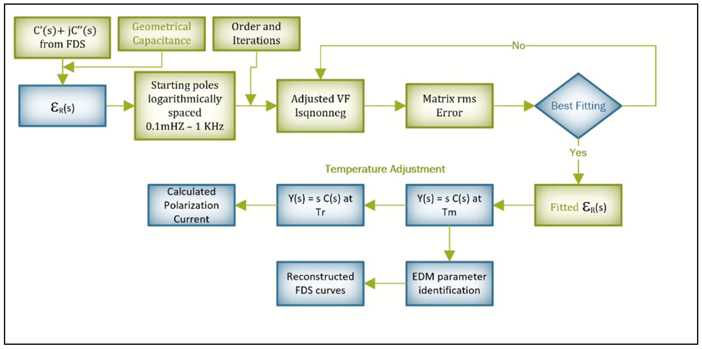
Figure 3.
Flowchart of parametrization and simulation algorithm.

Figure 4.
Measured and fitted dissipation factor.

Figure 5.
Measured and fitted complex capacitance curves.

Figure 6.
Measured and calculated polarization currents for transformers #3, #5, and #6.


Table 1.
Parameters of six new transformers under test.
| XFMR | 1 | 2 | 3 | 4 | 5 | 6 |
|---|---|---|---|---|---|---|
| MVA | 10 | 12.5 | 2.5 | 2 | 3.75 | 7.5 |
| KV Class | 27.6 | 34.5 | 38 | 46 | 69 | 115 |
| Fluid Type | FR3 | FR3 | Mineral | FR3 | Mineral | Mineral |
| %DF at 60 Hz and 20 °C | 0.35 | 0.37 | 0.32 | 0.41 | 0.32 | 0.29 |
| C at 60 Hz (pF) | 7457 | 9301 | 4185 | 4427 | 2686 | 2719 |
| Moisture (%) | 1.4 | 1.3 | 0.5 | 1.9 | 1.1 | 1.4 |
| Oil Cond (pS/m) | 9.98 | 7.67 | 0.872 | 13.2 | 2.05 | 0.844 |
Table 2.
Identified EDM parameters for six new transformers.
| XFMR #1 | XFMR #2 | XFMR #3 | |||||||
| Branch | (GΩ) | (nF) | (s) | (GΩ) | (nF) | (s) | (GΩ) | (nF) | (s) |
| 0 | 9.251 | 7.387 | 68.336 | 11.69 | 9.192 | 107.50 | 810.2 | 4.129 | 3345.3 |
| 1 | 0.003 | 0.051 | 0.0002 | 0.002 | 0.080 | 0.0001 | 0.002 | 0.040 | 0.0001 |
| 2 | 0.066 | 0.030 | 0.0020 | 0.040 | 0.042 | 0.0017 | 0.050 | 0.014 | 0.0007 |
| 3 | 0.705 | 0.029 | 0.0202 | 0.400 | 0.030 | 0.0121 | 0.375 | 0.015 | 0.0057 |
| 4 | 1.980 | 0.109 | 0.2154 | 2.474 | 0.039 | 0.0957 | 4.322 | 0.010 | 0.0449 |
| 5 | 1.318 | 5.015 | 6.6085 | 2.662 | 0.733 | 1.9509 | 24.41 | 0.021 | 0.5200 |
| 6 | 0.857 | 35.24 | 30.199 | 0.870 | 31.98 | 27.813 | 29.83 | 1.389 | 41.424 |
| 7 | 2.781 | 37.46 | 104.20 | 2.165 | 46.41 | 100.50 | 24.06 | 8.831 | 212.55 |
| 8 | - | - | 12.54 | 45.44 | 570.10 | 109.9 | 4.146 | 455.77 | |
| 9 | - | - | - | - | 218.7 | 8.688 | 1900.5 | ||
| XFMR #4 | XFMR #5 | XFMR #6 | |||||||
| Branch# | (GΩ) | (nF) | (s) | (GΩ) | (nF) | (s) | (GΩ) | (nF) | (s) |
| 0 | 29.05 | 4.360 | 126.69 | 71.94 | 2.664 | 191.63 | 88.45 | 2.696 | 238.42 |
| 1 | 0.002 | 0.049 | 0.0001 | 0.013 | 0.017 | 0.0002 | 0.006 | 0.018 | 0.0001 |
| 2 | 0.049 | 0.019 | 0.0009 | 3.993 | 0.001 | 0.0020 | 0.169 | 0.007 | 0.0012 |
| 3 | 0.424 | 0.021 | 0.0088 | 0.265 | 0.010 | 0.0027 | 0.971 | 0.012 | 0.0113 |
| 4 | 4.260 | 0.026 | 0.1090 | 2.931 | 0.007 | 0.0199 | 7.732 | 0.014 | 0.1098 |
| 5 | 3.673 | 1.460 | 5.3635 | 7.758 | 0.017 | 0.1288 | 17.27 | 0.066 | 1.1317 |
| 6 | 2.483 | 11.41 | 28.330 | 25.75 | 0.030 | 0.7649 | 53.13 | 1.093 | 58.081 |
| 7 | 17.45 | 9.275 | 161.89 | 16.13 | 1.306 | 21.064 | 834.0 | 0.171 | 142.86 |
| 8 | 104.2 | 9.995 | 1041.9 | 12.64 | 7.703 | 97.432 | 29.00 | 9.096 | 263.79 |
| 9 | - | - | - | 262.7 | 1.244 | 326.73 | 71.72 | 20.80 | 1492.4 |
| 10 | - | - | - | 71.39 | 10.80 | 771.11 | - | - | - |
Table 3.
AF of reconstructed FDS curves with the best order and iteration.
| XFMR | 1 | 2 | 3 | 4 | 5 | 6 |
|---|---|---|---|---|---|---|
| Best Order | 7 | 8 | 9 | 8 | 10 | 9 |
| Best Iteration | 2 | 3 | 5 | 3 | 3 | 5 |
| rms error | 0.29 | 0.02 | 1.13 | 0.48 | 2.22 | 0.69 |
| (%) | 99.94 | 99.80 | 99.74 | 99.83 | 99.71 | 99.74 |
| (%) | 99.84 | 99.70 | 99.78 | 99.84 | 99.72 | 99.87 |
| (%) | 99.37 | 99.30 | 98.97 | 98.58 | 98.25 | 97.63 |
Publisher’s Note: MDPI stays neutral with regard to jurisdictional claims in published maps and institutional affiliations. |
© 2022 by the authors. Licensee MDPI, Basel, Switzerland. This article is an open access article distributed under the terms and conditions of the Creative Commons Attribution (CC BY) license (https://creativecommons.org/licenses/by/4.0/).
Share and Cite
MDPI and ACS Style
Hernandez, G.; Ramirez, A. Dielectric Response Model for Transformer Insulation Using Frequency Domain Spectroscopy and Vector Fitting. Energies 2022, 15, 2655. https://doi.org/10.3390/en15072655
AMA Style
Hernandez G, Ramirez A. Dielectric Response Model for Transformer Insulation Using Frequency Domain Spectroscopy and Vector Fitting. Energies. 2022; 15(7):2655. https://doi.org/10.3390/en15072655
Chicago/Turabian StyleHernandez, Giovanni, and Abner Ramirez. 2022. "Dielectric Response Model for Transformer Insulation Using Frequency Domain Spectroscopy and Vector Fitting" Energies 15, no. 7: 2655. https://doi.org/10.3390/en15072655
Note that from the first issue of 2016, this journal uses article numbers instead of page numbers. See further details here.