Abstract
A complex structural geology generally leads to significant consequences for hydrocarbon reservoir exploration. Despite many existing wells in the Kadanwari field, Middle Indus Basin (MIB), Pakistan, the depositional environment of the early Cretaceous stratigraphic sequence is still poorly understood, and this has implications for regional geology as well as economic significance. To improve our understanding of the depositional environment of complex heterogeneous reservoirs and their associated 3D stratigraphic architecture, the spatial distribution of facies and properties, and the hydrocarbon prospects, a new methodology of three-dimensional structural modeling (3D SM) and joint geophysical characterization (JGC) is introduced in this research using 3D seismic and well logs data. 3D SM reveals that the field in question experienced multiple stages of complex deformation dominated by an NW to SW normal fault system, high relief horsts, and half-graben and graben structures. Moreover, 3D SM and fault system models (FSMs) show that the middle part of the sequence underwent greater deformation compared to the areas surrounding the major faults, with predominant one oriented S30°–45° E and N25°–35° W; with the azimuth at 148°–170° and 318°–345°; and with the minimum (28°), mean (62°), and maximum (90°) dip angles. The applied variance edge attribute better portrays the inconsistencies in the seismic data associated with faulting, validating seismic interpretation. The high amplitude and loss of frequency anomalies of the sweetness and root mean square (RMS) attributes indicate gas-saturated sand. In contrast, the relatively low-amplitude and high-frequency anomalies indicate sandy shale, shale, and pro-delta facies. The petrophysical modeling results show that the E sand interval exhibits high effective porosity (∅eff) and hydrocarbon saturation (Shc) compared to the G sand interval. The average petrophysical properties we identified, such as volume of shale (Vshale), average porosity (∅avg), ∅eff, water saturation (SW), and the Shc of the E sand interval, were 30.5%, 17.4%, 12.2%, 33.2% and, 70.01%, respectively. The findings of this study can help better understand the reservoir’s structural and stratigraphic characteristics, the spatial distribution of associated facies, and petrophysical properties for reliable reservoir characterization.
1. Introduction
The recent global increase in fuel demand has increased hydrocarbon production at established reservoirs [1,2]. According to the United States Energy Information Administration (USEIA), Pakistan may have over 9 billion barrels of oil and 105 trillion cubic feet of natural gas (including shale gas) reserves [3]. Pakistan’s gas fields are only expected to last for about another 20 years at the most due to heavy industrial usage. Therefore, many recent works on the Lower Indus Basin (LIB) are focused on unconventional resources such as shale gas and coal seam gas [4,5,6]. However, focused characterization and re-evaluations of already-discovered petroleum systems are also required to evaluate reservoirs’ abilities to meet the hydrocarbon requirements [7].
Reservoir characterization is a scheme that quantifies the physical and fluid properties of rock [8,9,10,11,12]. It also involves an understanding of reservoir structure, sedimentological heterogeneity, facies, and the quantity of hydrocarbon that exist in structural traps driven by tectonic movements, discontinuities such as faults, folds, anticlinal structures, horst and graben pop-up geometries, and duplex structures [13,14,15,16,17,18]. Advancements in 3D seismic data analysis and borehole geophysics have made it possible to characterize structural and stratigraphic features and their associated petrophysical properties with high reliability and precision, thereby reducing the risks associated with hydrocarbon exploration [19,20].
The development of three-dimensional structure models (3D SMs) is essential for reservoir description, e.g., true structural dip, fault system models (FSMs), up-dip hydrocarbon migration pathways, and quantitative geometric characterization in 3D space [21,22]. Three-dimensional structural modeling (3D SM) is divided into entity-based modeling and volume-based modeling (VBM) [23,24,25,26,27,28]. The former develops 3D SMs using a combination of four different geometric entities, i.e., point, line, surface, and body. It emphasizes the shape of geological structures and the relationship among geological bodies [29]. The latter subdivides the 3D space into discrete fields by regular or irregular voxels and emphasizes the spatial distribution of geophysical and geochemical properties. With the continuous development of reservoir geological modeling technology, the VBM, objective function, variation function, multipoint geostatistics, and static geological modeling with knowledge-driven methodology have been widely applied, significantly promoting the development and technology of 3D reservoirs geological modeling [30,31,32,33,34,35,36]. However, VBM is a step-change reservoir geological modeling technique that creates horizons based on depositional sequence instead of considering horizons as discrete surfaces [2,13,37].
Identifying reservoir facies and properties using seismic attributes and petrophysical analyses play an essential role in reservoir characterization. Reservoir facies classification and properties evaluation can be achieved via laboratory studies on core plugs, which are costly and time-consuming. However, seismic attributes can be used for stratigraphic-based basin depiction within a composite deposition-based structure and classify reservoir facies, thereby increasing the rate for adequate reservoir characterization. Seismic attributes, such as dip magnitude, edge enhancement, variance edge, sweetness, and root mean square (RMS) amplitude, are essential tools for delineating structural and stratigraphic characteristics, lithofacies changes, and hydrocarbon potential zones [19,38,39]. On the other hand, petrophysical analysis based on well logs offers practically continuous reservoir properties, e.g., lithology, the volume of shale (Vshale), average porosity (∅avg), effective porosity (∅eff), water saturation (SW), and hydrocarbon saturation (Shc). The proper analysis of these properties can significantly improve the ability to distinguish hydrocarbon-bearing zones [18,20,40,41].
The Middle Indus Basin (MIB) and Lower Indus Basin (LIB) are well known for hydrocarbon exploration in Pakistan [40]. The Kadanwari field in MIB is a significant hydrocarbon-producing field, with the early–late Cretaceous Lower Goru formation (LGF) acting as the potential reservoir. The previous studies conducted on the Kadanwari field were based on the assessment and development of the 2D fault system, porosity prediction [42], formation evaluation [40,43], and impact of diagenesis on reservoir quality prediction [44].
A systematic review of prospective observational studies found that the Kadanwari field in MIB has not yielded sufficient results for understanding the complex structural depositional environment [45]. Moreover, the distribution of key petrophysical properties and facies in the Kadanwari field are difficult to predict due to fluctuating deltaic conditions, mutable geological influences, varying hydrocarbon concentrations, regional tectonic settings, and changes in geometries. However, comprehensive research on the structural characteristics and associated tectonic extensional fault system models (FSMs) and the evaluation of reservoir characteristics and sweet spots for future drillings in the Kadanwari field is still missing.
This study, therefore, aims at evaluating the complex and heterogeneous depositional environment broadly comprised of structural and stratigraphic characteristics, distribution of associated facies, and petrophysical properties for reliable reservoir characterization, which was lacking in the previous studies. This was achieved by utilizing three-dimensional structural modeling (3D SM) and joint geophysical characterization (JGC) using seismic and well logs data. In this study, 3D SM and JGC have made novel contributions and facilitated a clearer representation of the complex and heterogeneous depositional environments, with the lateral and horizontal structural extent of reservoir horizons, FSMs (including fault geometry and orientation in 3D space), spatial facies, reservoir properties (e.g., lithology, Vshale, ∅avg, ∅eff, SW, and Shc), and direct hydrocarbon indicators (DHIs). In short, our presented study is crucial to characterize and evaluate reservoirs’ geometrical characteristics, facies, and properties, in order to reduce uncertainties and improve the success rate of future exploration and development plans pertaining to hydrocarbons in the study area, as well as potentially in other regions around the world.
2. Background Geology
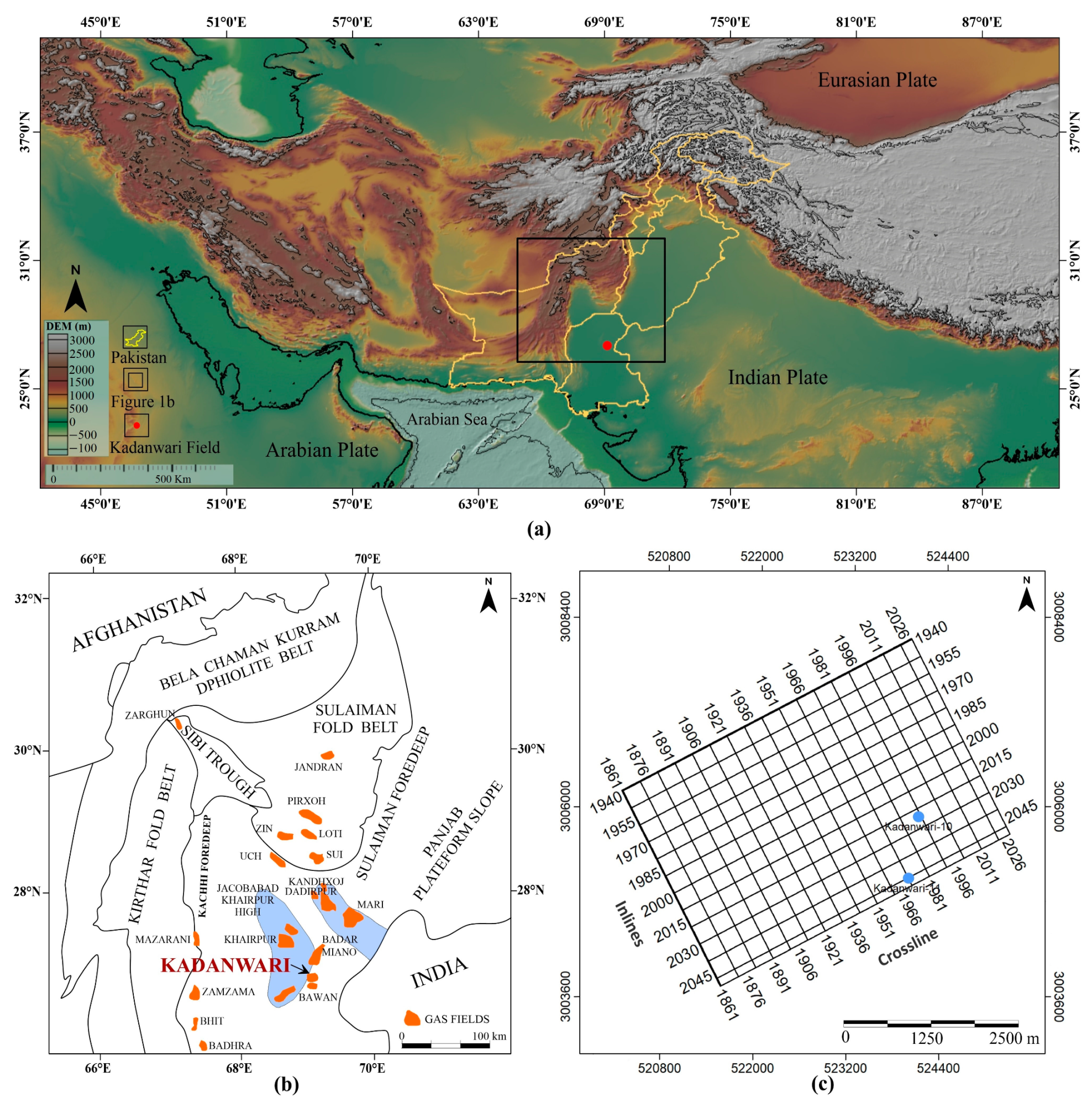
Pakistan is located at the triple junction of the Indian, Eurasian and Arabian plates (Figure 1a). During the middle/late Jurassic to early Cretaceous, the Indian plate rifted away from the Gondwana landmass, forming an island continent that drifted northwards into the Tethyan Ocean [46]. This tectonic event predominantly influenced the structures and sedimentation of the MIB and LIB, which could have resulted in NE—SW to N—S rift systems. The Kadanwari field is located in the District Khairpur of Sindh Province, southeast MIB, a prolific gas-prone basin in Pakistan (Figure 1b). The latitude of the study area ranges from 27°04′83″ N to 27°07′12″ N, and its longitude varies from 69°12′98″ E to 69°17′57″ E. Tectonically, the Kadanwari field lies between two extensive regional highs, i.e., the Mari-Kandhkot High and the Jacobabad-Khairpur High (Figure 1b). In the east, it is bounded by the Indian shield; in the north by the Sargodha high; in the west by the fold and thrust belt of the Kirthar and Sulaiman Ranges, and in the south by the Jacobabad-Khairpur High [7,45,46,47]. Three tectonic events were responsible for the structural configuration of the study area, i.e., the late Cretaceous uplift and erosion, the late Paleocene wrench faulting, and the late Tertiary to Quaternary uplift/inversion of Jacobabad High (Figure 1b) [46]. The Jacobabad-Khairpur High was a primary contributor to the study area’s structural traps and surroundings [45,47]. The final tectonic event of the late Tertiary to Quaternary was an inversion of the Jacobabad-Khairpur High, which significantly affected the Kadanwari area [45,46]. In the Kadanwari field and its surroundings, the trapping mechanism is a complex combination of structural dip, sealing faults, and loss of reservoir quality to the north. The Kadanwari field consists of several low-relief faults, forming dip closures in the subsurface and providing a stratigraphic trapping component [7,45]. The fault dip closures and the wrench faults are particularly significant as they divide the Kadanwari field into reservoir compartments [40].

Figure 1.
(a) Location of the study area; (b) generalized tectonic map with the location of major oil- and gas-producing fields in the study area, bounded by other gas fields, modified from [49]; (c) the base map shows the orientation and general information of the 3D seismic lines and wells in the Kadanwari field, MIB, Pakistan.
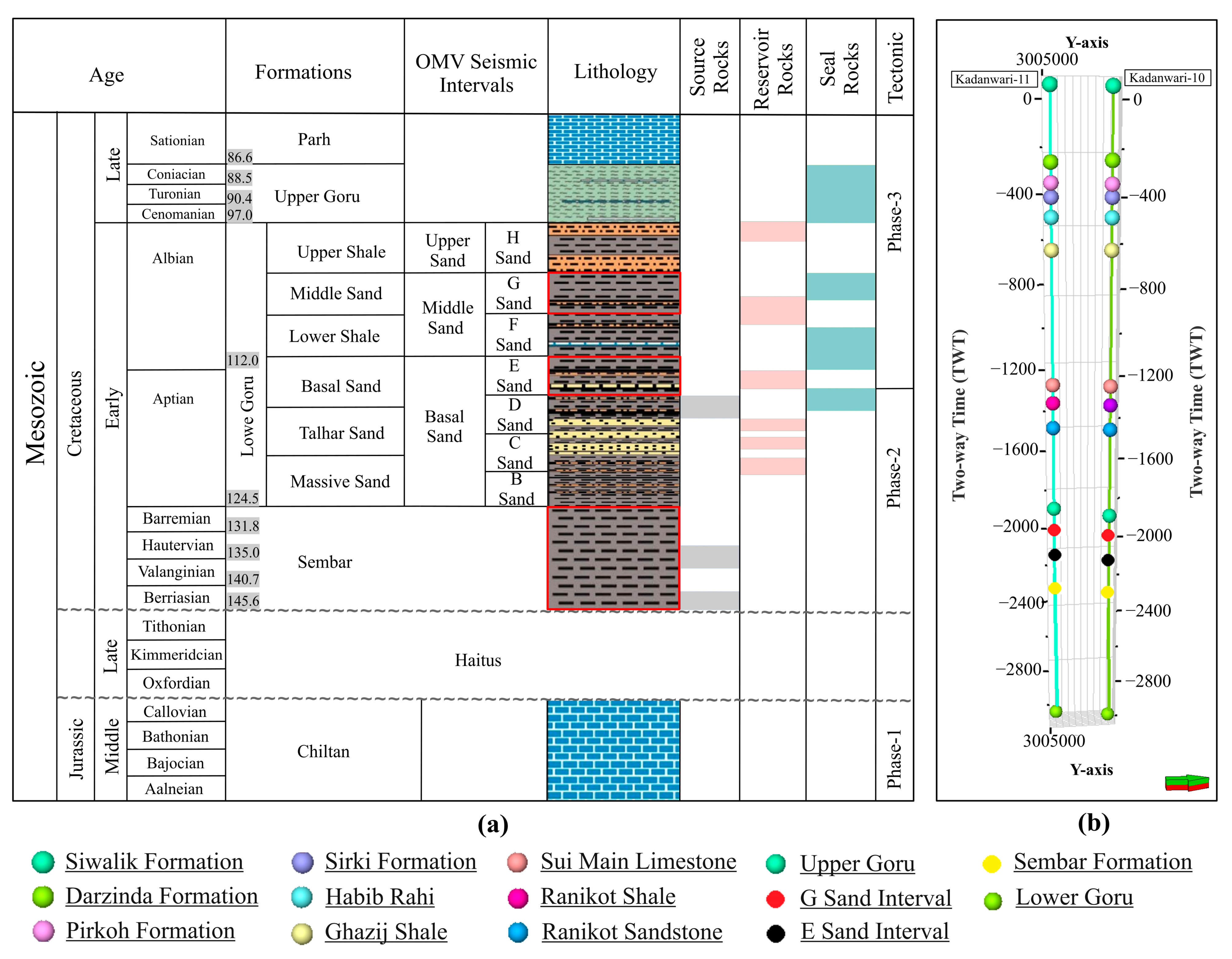
The lithology stack of MIB is depicted in Figure 2a, highlighting the basin fill sedimentary deposits. The lithostratigraphic columns show the rock units encountered in the Kadanwari-10 and Kadanwari-11 wells (Figure 2b). According to [48], the shales of the Sember Formation serve as the source rock for the regional petroleum systems of the MIB. However, the reservoir sections (e.g., G and E sands) in the Kadanwari field belong to the lower Goru sand (the Cretaceous age), while the sealing is provided by the upper Goru shaly sequence [43].
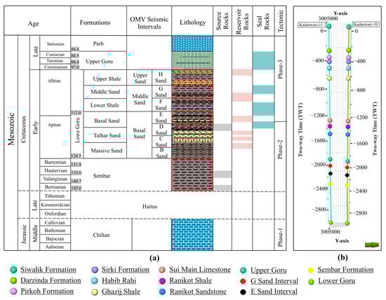
Figure 2.
(a) Generalized stratigraphic column of the study area, modified from [48]; (b) lithostratigraphic columns showing the rock units encountered in Kadanwari-10 and Kadanwari-11 wells.
3. Material and Methods
3.1. Datasets Description and Processing
A vast volume of seismic reflection data was acquired from the MIB, Pakistan, to facilitate hydrocarbon exploration activities at different times, from the 1970s up to the modern-day [7]. The Pakistan branch of OMV (www.omv.com, Vienna, Austria) recently began a new exploration phase in the Kadanwari field by conducting a 3D seismic survey. The seismic data used in this study are 3D post-stack time migrated seismic reflection cubes stored in the SEG-Y format, wherein approximately 116 seismic inlines and approximately 181 cross-lines were used. The geometric information, e.g., total coverage area, inline interval, crossline interval, and time slice range of available 3D seismic data, were 12 km2, 24.17, 25.17, and 1800–2600 (ms), respectively. The well logs data comprise lithology, resistivity, and porosity logs (e.g., GR, SP, LLD, LLS, MSFL, RHOB, NPHI, and DT) of the Kadanwari-10 and Kadanwari-11 wells (Table 1). The available 3D seismic data and well log data were collected from the Landmark Resources (LMKR) (www.lmkr.com, Calgary, Canada) upon the request of the Directorate General of Petroleum Concessions (DGPC) (www.mpnr.gov.pk, Islamabad, Pakistan); which are available to the public domain and can be utilized for scientific and research purposes. The dataset quality was first checked and harmonized in a clearly defined database. Accordingly, a base map of the 42-N Trans-Mercator Macrocosm (UTM) zone was created using navigation and SEG-Y records to determine the orientation (dip or strike) and location of seismic lines and wells (Figure 1c).

Table 1.
Metadata of the utilized well logs and their uses in this study.
3.2. Methods
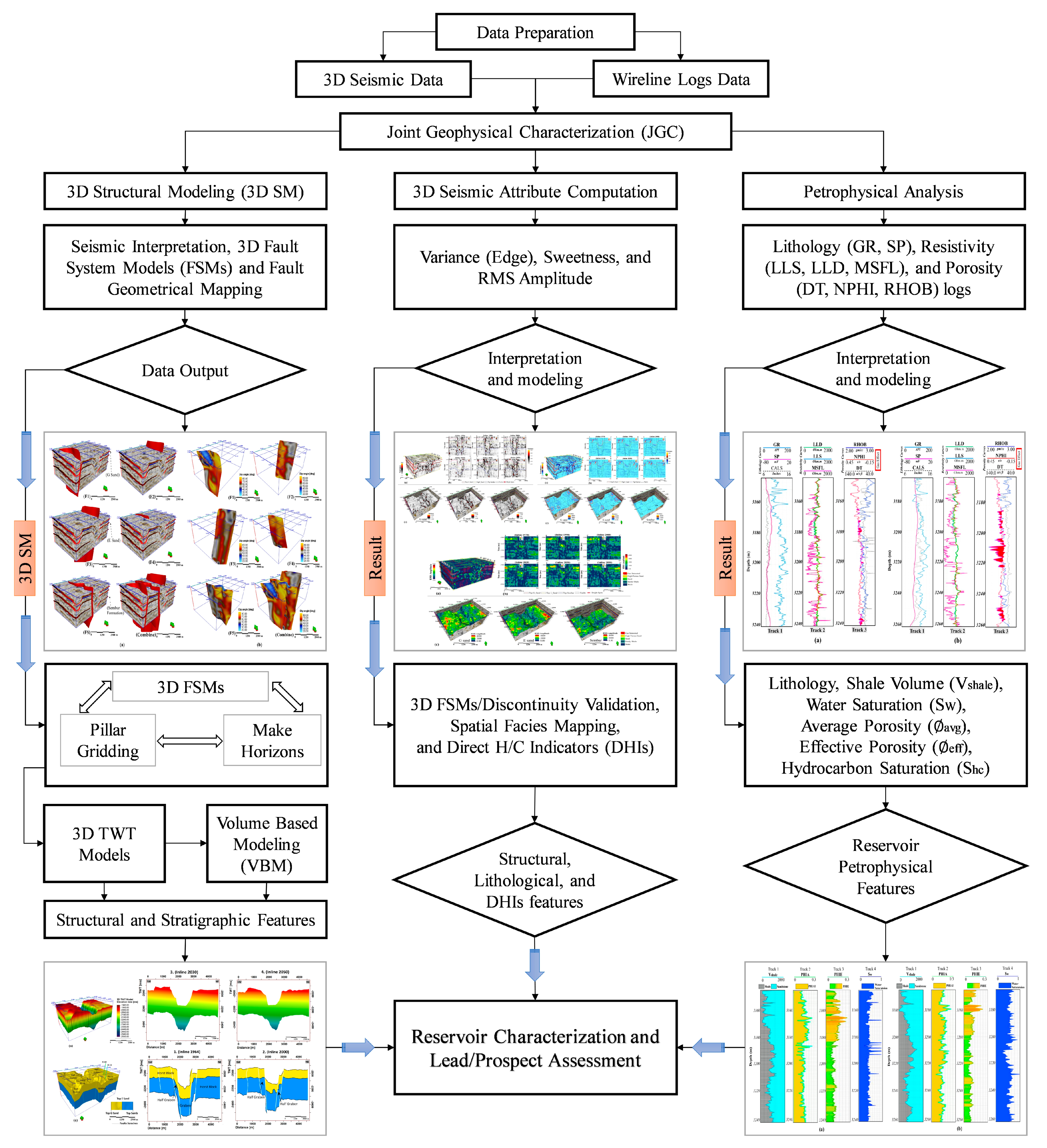
In this study, three-dimensional structural modeling (3D SM) and joint geophysical characterization (JGC) use an integrated 3D SM approach, involving structurally constrained geological models and seismic attribute implications and petrophysical properties that significantly enhance the understanding of the reservoir characteristics leading to reliable reservoir assessment. Figure 3 shows the complete workflow of the present case study. Firstly, seismic and well log data interpretation was carried out, which involves synthetic seismogram generation, and extracting and interpreting specific stratigraphic interfaces (geological period) and faults as geometric features in 2D cross-sectional (i.e., vertical) slices of a 3D seismic volume. Secondly, 3D FSMs and their attribute models such as dip angles, fault rose diagram and histogram were constructed to evaluate the fault mechanics and geometric distribution. Thirdly, 3D SMs of the early Cretaceous stratigraphic sequence were constructed using the VBM algorithm, incorporating all geometrical definitions (e.g., constraints from well tops, geologic horizons, and FSMs). Fourthly, several seismic attributes such as variance edge, sweetness, and RMS amplitude were incorporated into the 3D seismic data, which involves extracting the corresponding qualitative and quantitative geological features to validate the interpreted spatial forecasts of the geological structure, and to then evaluate the lithofacies distribution and direct hydrocarbon indicators (DHIs). Finally, petrophysical modeling based on various well logs (CALI, GR, SP, LLD, LLS, MSFL, DT, NPHI, and RHOB, explained in Table 1) was performed to determine the reservoir properties (e.g., lithology, Vshale, ∅avg, ∅eff, SW, and Shc).
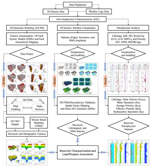
Figure 3.
Workflow highlighting various steps and methods employed in this study for reservoir characterization and prospect assessment of the Kadanwari field, MIB, Pakistan.
3.2.1. Seismic Data Interpretation
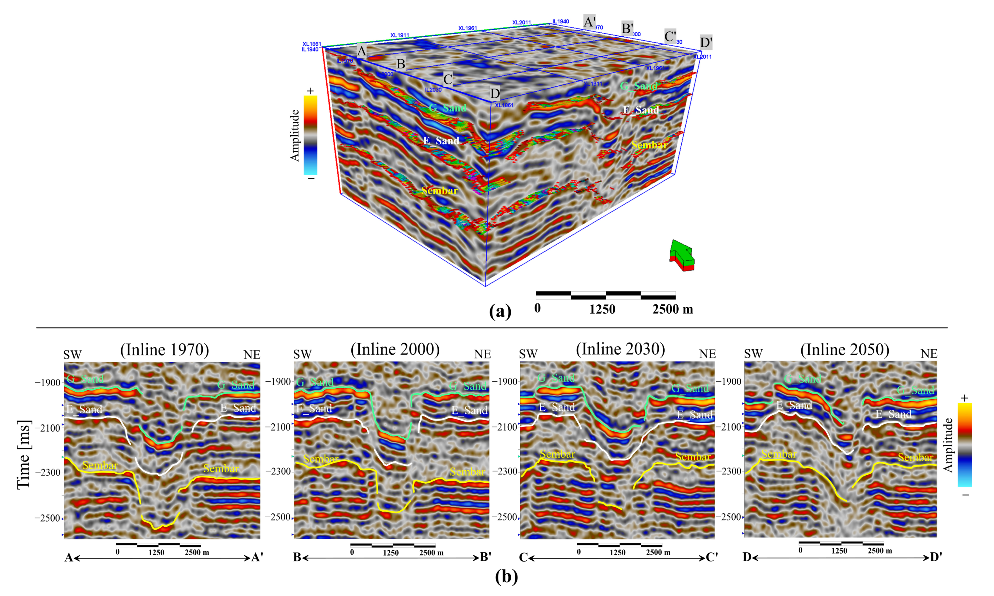
Seismic interpretation in this study is focused on a particular area of interest within the two-way time (TWT) range of −1800 to −2600 (ms) (Figure 4). Depending on the seismic reflection discontinuities and terminations, manual horizon picking followed by seeded horizon auto-tracking was adopted to interpret the target horizons on 2D cross-sectional (i.e., vertical) slices of a 3D seismic volume (Figure 4a). In the middle parts of the seismic cross-sections, the reflections are mostly moderately chaotic and difficult to correlate due to the complexity of the geology and faults resulting from tectonic compression (Figure 4b). The modeling step of the seismic interpretation involves 3D TWT contour surfaces construction. Consequently, 3D TWT contour surfaces were constructed by marking the tops of each stratigraphic interface on the extended 3D seismic volume. The smooth function was then applied to the generated surfaces at three iteration levels to produce geologically reasonable stratigraphic surfaces. These 3D TWT contour surfaces were then used to interpret the prevailing structural trends in the study area via conventional methods.
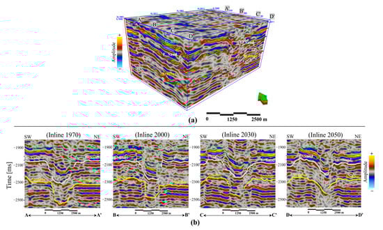
Figure 4.
(a) 3D time-seeded horizon auto-tracking; (b) amplitude display of vertical time inline cross-sections (e.g., 1970, 2000, 2030, and 2050) in the SW to NE direction, showing horizon interpretation. Mint green, white, and yellow colors represent the lateral extent of the G sand interval, the E sand interval, and the Sembar Formation, respectively.
3.2.2. Three-Dimensional Structural Modeling (3D SM)
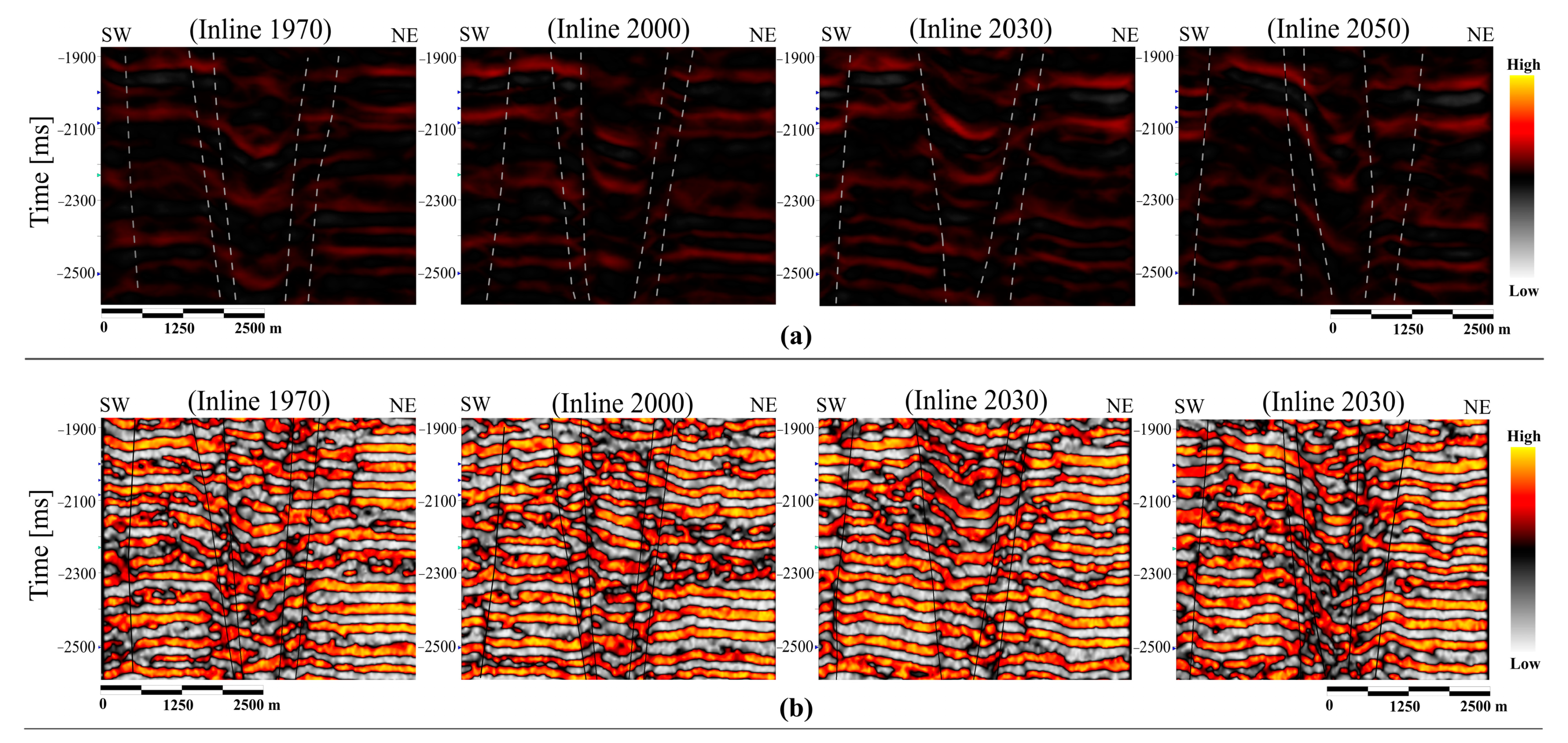
Employing 3D fault system modeling (FSM) in seismic analysis is a crucial step to constrain horizon interpretation [21,50]. One recent significant advance in FSM is the rendering available of 3D seismic data that provide detailed images of large volumes of rock and the often-complex 3D fault networks [51]. Meanwhile, most seismic datasets have signal disturbance zones, particularly in highly faulted areas. Furthermore, the discontinuities in seismic reflectors can be poorly resolved, resulting in the approximate localization or misinterpretation of faults. However, seismic discontinuities can be more clearly defined if the detection is based on multiple attributes and suitable filters [51,52]. Therefore, in this study, before proceeding to the 3D FSM, the precision of the geologic fault boundaries was assessed first for accuracy using dip magnitude and seismic edge enhancement attributes (Figure 5). Accordingly, the dominance of a normal fault system was inferred in the dip magnitude and edge enhancement cross-sections by aligning reflector discontinuities and degree of displacement. In the modeling phase, the fault surfaces were constructed by employing the fault polygon in PetrelTM software for each type of fault with various geometrical structures. Finally, 3D FSMs and their attribute models (e.g., dip angle, fault rose diagram and histogram) were constructed to evaluate the fault system’s geometric distribution and mechanics within the early Cretaceous stratigraphic sequence.
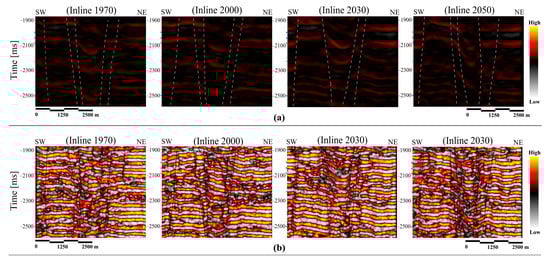
Figure 5.
Fault system tracing and interpretation in the Kadanwari field using resemble brittle deformation features (seismic reflection discontinuities, terminations, and amount of displacement) on (a) dip magnitude and (b) seismic edge enhancement attributes cross-sections.
Three-dimensional SM aims to better image and understand complex reservoirs’ geological structures. The local tectonics of the Kadanwari field in MIB have resulted in various structural deformations that produce many uncertainties when assessing the reservoirs’ 3D structural framework [7]. Understanding such deformations can be better achieved via 3D SM using relevant algorithm models, e.g., the volume-based modeling (VBM) approach in the PetrelTM software based on inferred seismic data integrated with borehole information [50,53,54]. Traditional modeling methods generally involve the oversimplification of geological settings; however, grid-generated VBM captures a realistic reservoir architecture [2]. This can be easily transferred into the dynamic realm, providing a better understanding of the reservoir for future field management and development activities [50]. In this study, 3D SM based on the VBM approach was performed in three main steps (e.g., fault modeling, pillar gridding, and horizon creation).
3.2.3. Three-Dimensional Seismic Attribute Analysis
The seismic attributes were computed via mathematical manipulation of the original seismic data to highlight specific geological, physical, or reservoir properties [50,55]. Variations in the amplitude, phase, frequency, and bandwidth of the seismic waves were subsequently used to validate the spatial forecasts of the geological structure and to evaluate the spatial distribution of the facies and the DHIs in the G sand interval, the E sand interval, and the Sember Formation time windows.
The variance edge attribute can visualize seismic amplitude discontinuities related to faulting or stratigraphy. It delineated the prominent faults and seismic amplitude discontinuity in both the horizon slices and the vertical seismic profiles, thereby validating the manual interpretation of faults. The sweetness attribute was applied to both horizon slices and vertical seismic profiles to identify sweet spot zones that are hydrocarbon-prone. It can be defined as the reflection strength (instantaneous amplitude) divided by the square root of the instantaneous frequency. The high sweetness anomalies highlight a seismic signal’s high amplitudes and low-frequency contents and vice versa. Therefore, combining these two physical quantities helps distinguish sand bodies from shale and predicted gas-prone zones [56]. The RMS amplitude attribute was also applied to both horizon slices and vertical seismic profiles to measure amplitude anomalies to identify the spatial distribution of facies and DHIs at the G and E sand reservoir intervals. The RMS amplitude computes the square root of the sum of squared amplitudes divided by the number of samples within the window used [19].
3.2.4. Petrophysical Modeling
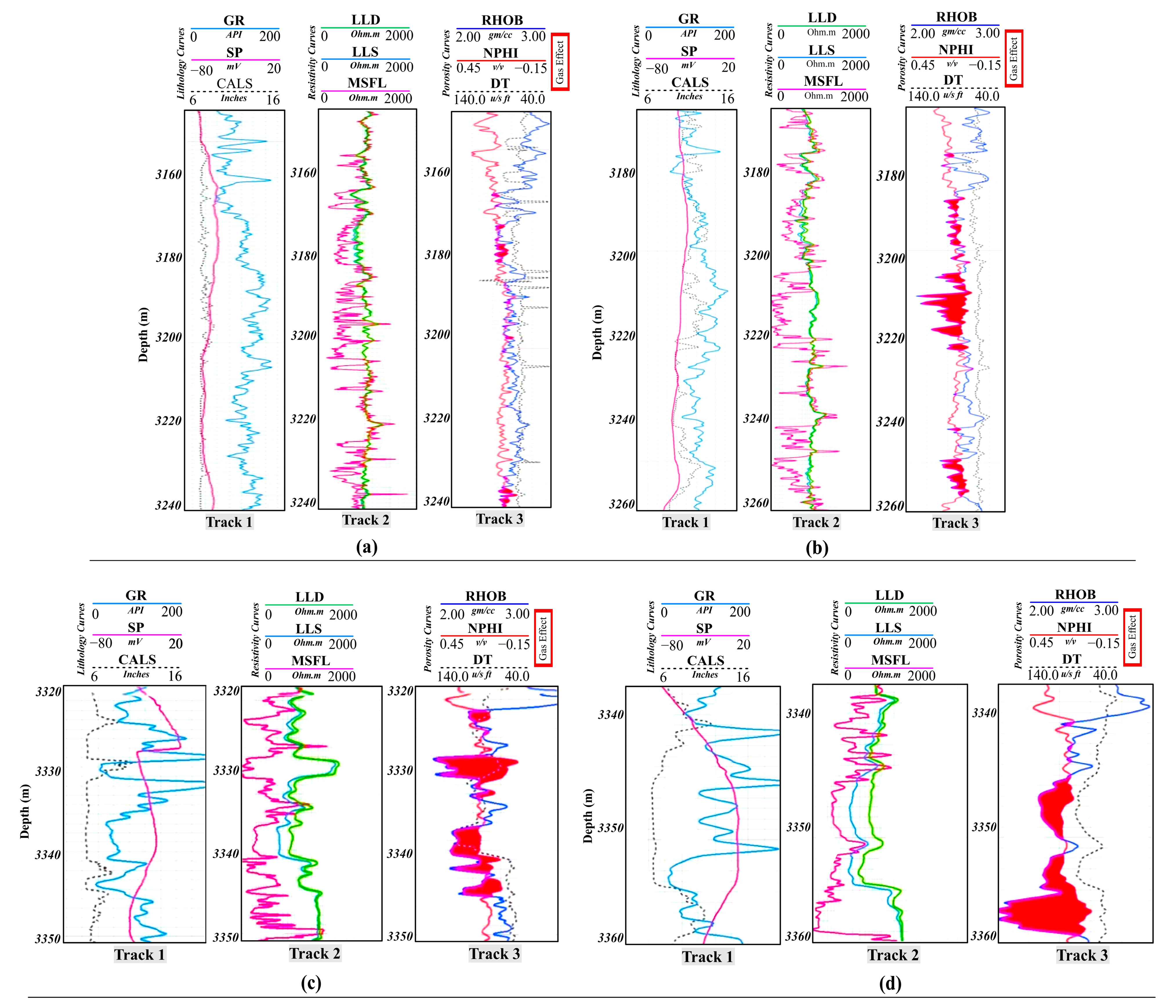
Petrophysical modeling is critical in a reservoir study because it represents a primary input data source for integrated reservoir characterization and resource evaluation [54,57]. This study performed petrophysical modeling based on well log data and internal geological reports to evaluate the G and E sand reservoir intervals’ properties, e.g., lithology, Vshale, ∅avg, ∅eff, SW, and Shc (Table 1). Successful evaluation of these properties is necessary when determining the hydrocarbon potential of a reservoir system. The detailed plots of the well log curves and their depth ranges within the G and E sand reservoir intervals are shown in Figure 6. These log curves express the physical motifs of the stacked geological strata as a function of depth, which can help identify lithologies and porosities, and differentiate between porous and non-porous rocks and pay zones.
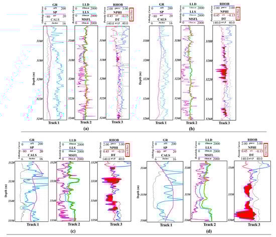
Figure 6.
Input conventional log curves for the petrophysical modeling of the G sand interval in the (a) Kadanwari-10 (b) and Kadanwari-11 wells and for E sand interval in the (c) Kadanwari-10 (d) and Kadanwari-11 wells.
The following five key steps were followed to evaluate the reservoirs’ fundamental properties.
- (1)
- Volume of Shale (Vshale)—The presence of shale in the productive zone severely impacts the petrophysical properties and can cause a reduction in the ∅eff, ∅avg, and permeability [58]. We used the GR log technique for Vshale estimation by firstly estimating the gamma ray index (IGR). The IGR was initially adopted using Equation (1) to estimate Vshale, utilizing the GRlog in track 1 of Figure 6. Secondly, to obtain a realistic Vshale estimation without overestimating the content of shale (first-order approximation: Vshale = IGR), a non-linear relationship (Equation (2)) proposed by Dolan was employed [59].where IGR stands for gamma ray index, GRlog shows the reading of the gamma ray log, GRmin and GRmax are the lower and upper limits of the GRlog value in shale, respectively.
- (2)
- Average Porosity (∅avg)—Total porosity or ∅avg represents all the voids or pore spaces of the rock, including interconnected and isolated pores and pore spaces occupied by clay-bound water [2]. In this study, DT, RHOB, and NPHI logs that are sensitive to sedimentary micro-facies were selected to calculate ∅avg, by which process the conventional logging responses of the G and E sand reservoir intervals can be summarized (Figure 6).The DT log measures the sound waves’ traveling times in the rock unit. The sound waves in the rock unit depend on the shape, matrix material, and cementation (Equation (3)). Accordingly, the Sonic–Raymer (SR) porosity model was used to evaluate sonic porosity (∅S) (Equation (4)) [40].where ∅S represents sonic porosity, tlog represents the log reading in μsec/m, tm represents the matrix interval transient time, ∆tlog represents the formation interval transient time in μsec/m, and ∆tm represents formation fluids’ interval transient time in μsec/m.The density porosity (ϕD) was calculated using the RHOB log via Equation (5) [2].where represents the density of the matrix, represents the fluid density, and is the bulk density.The NPHI log measures the neutron porosity (∅N) by assuming that the pores are filled with fluid. Therefore, it measures the hydrogen concentration and energy loss. The ∅N can be expressed via Equation (6).where is the neutron-derived porosity, a and b are constants, and N is the neutron count in the formation intervals. In addition, the density–neutron cross-plot in track 4 in Figure 6 determines the cross-over gas effects.After identifying the porosities (e.g., ∅S, ∅D, and ∅N) from the DT, RHOB, and NPHI logs, Equation (7) was used to calculate ∅avg.
- (3)
- Effective Porosity (∅eff)—The ∅eff was calculated using Equation (8) [40,43].where ∅avg represents the average porosity, and Vshale is the shale content in volume units.
- (4)
- Water Saturation (SW)—The Poupon–Leveaux Indonesian (PLI) model is one of the best models for estimating SW in a shaly sand reservoir [60]. In this study, the constraints of Vshale (Equation (2)) and ∅eff (Equation (8)), and the resistivity variation in Vshale and water formation, were subsequently integrated using the PLI model, as in Equation (9), to determine SW.where is the true resistivity of the formation obtained from the LLD log response, is the resistivity variation in the , and is the resistivity of water formation.
- (5)
- Hydrocarbon Saturation (Shc)—The Shc was calculated by subtracting the percentage of pore volume occupied by Sw from 1; the remaining percentage pore volume gives the Shc (Equation (10)).
4. Results
4.1. Stratigraphic Interfaces Interpretation
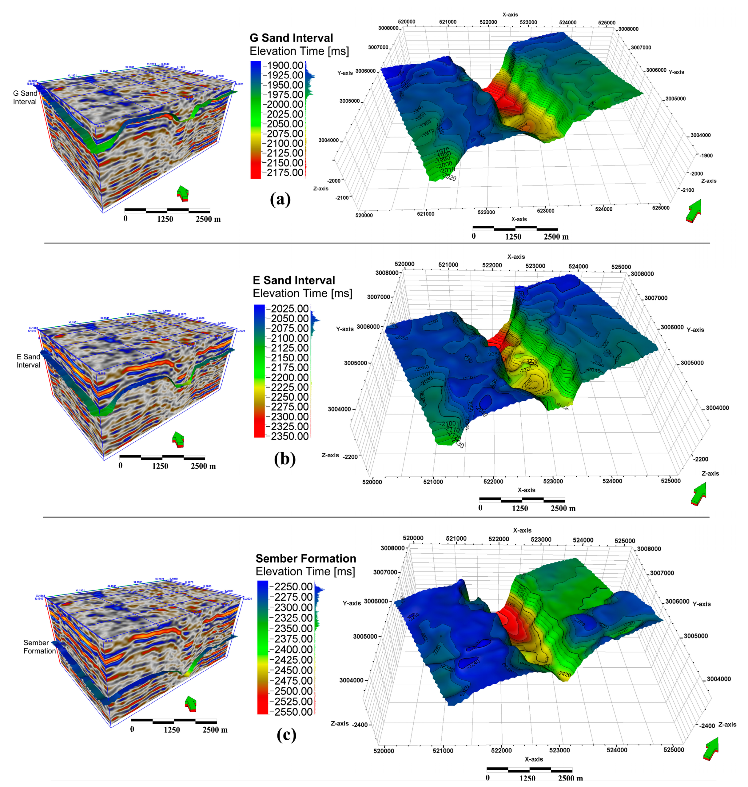
The interpretation of the stratigraphic interfaces of the early Cretaceous sequence is integrated into an internally consistent 3D workflow, which is easy to incorporate and use to form conclusions that exceed known points by constraining 3D structural models. The interpreted cross-sectional (i.e., vertical) slices of a 3D seismic volume show the displacement and deformation of the stratigraphic interface (Figure 4b). The structural variations in the stratigraphic interfaces are predicated primarily on the TWT contour surfaces because contour lines connect the same elevation; this is why they are essential tools for analyzing and interpreting seismic data. The time surfaces plot the TWT of seismic signals from the surface to the horizon and reflect the interpreted stratigraphic interface’s distribution. In Figure 7, the TWT surfaces indicate the extension and propagation of the regional stratigraphic structure in the subsurface. The TWT values of the interpreted stratigraphic interfaces decrease towards the central part of the field, which gives rise to structural highs in the southwestern and southeastern portions. The southwestern and southeastern portions of the interpreted stratigraphic interfaces are structurally high; hence, this is a region of interest for hydrocarbon exploration. The minimum, mean and maximum TWT variations of the G sand interval, the E sand interval, and the Sembar Formation in the southwestern and southeastern transect are presented in Table 2.
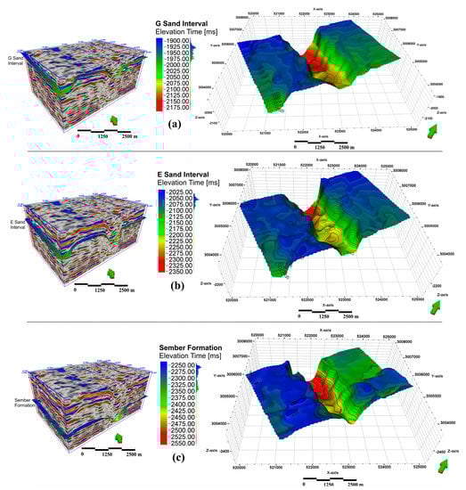
Figure 7.
Three-dimensional TWT contour surfaces of the stratigraphic interfaces show different structural distributions: (a) TWT top surface of the G sand interval; (b) TWT top surface of the E sand interval; (c) TWT top surface of the Sembar formation in 3D space.
Table 2.
Minimum, mean, and maximum TWT variations of the stratigraphic interfaces in the study area.
4.2. Three-Dimensional Fault System Models (3D FSMs)
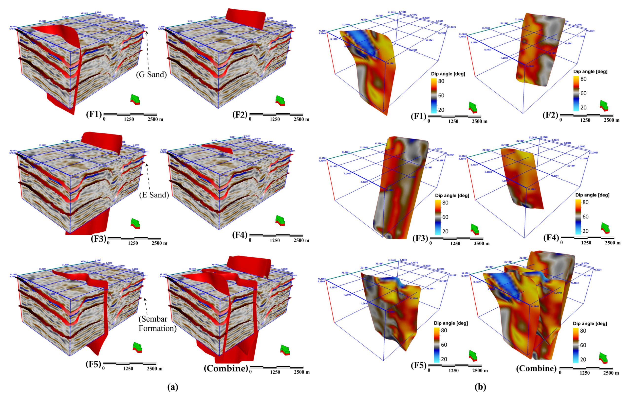
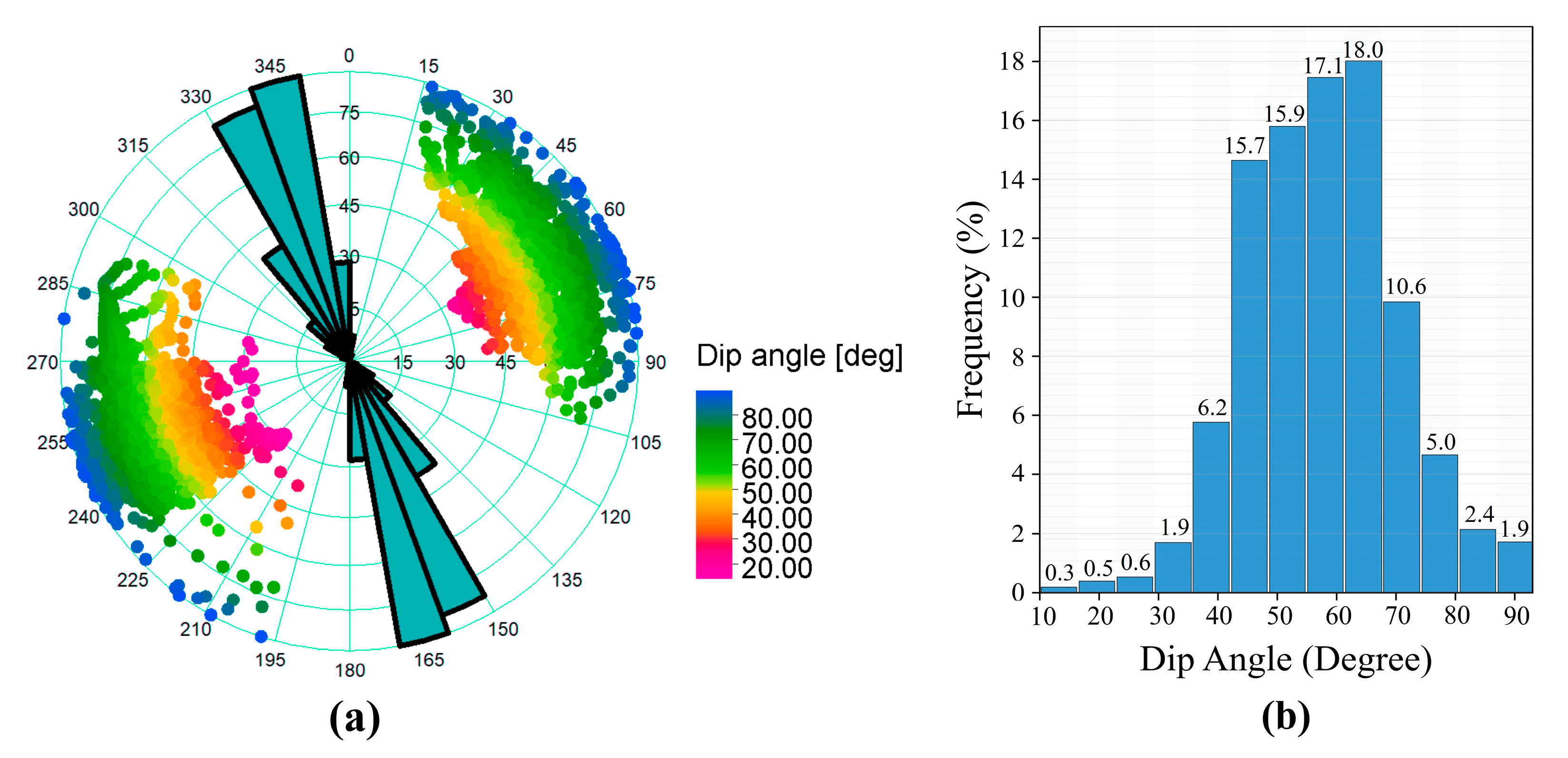
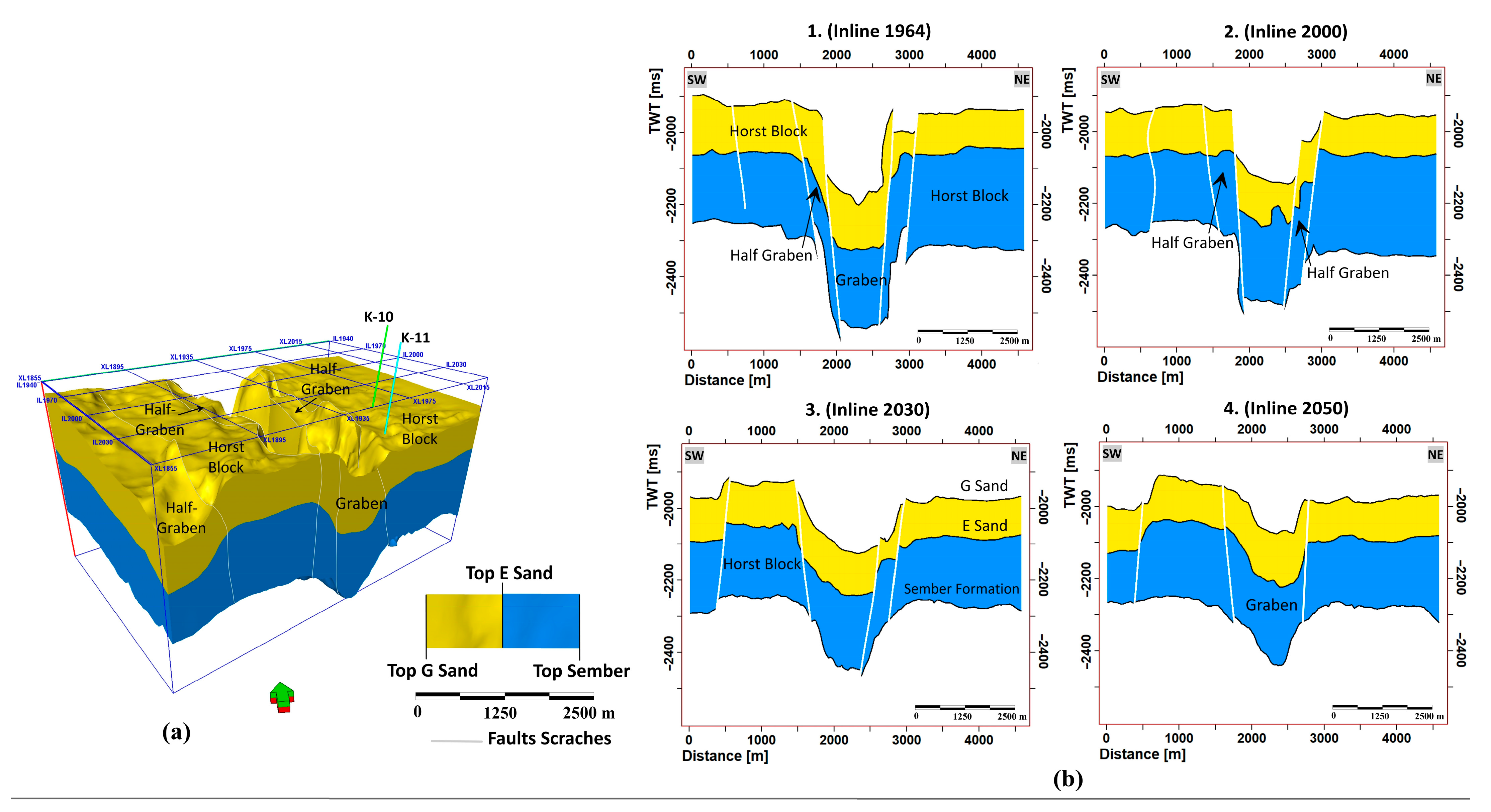
The study area’s complex and composite subsurface morphology resulted from multiple episodes of tectonic activity. Multi-stage tectonic movements contribute to the intersection of faults formed simultaneously or at different stages of tectonic movement (Figure 8a). These faults occurred during various phases of adjustment and deformation, along with the structure inversion and loss of reservoir quality in the Kadanwari field, MIB. In order to effectively represent the spatial distribution of the fault system and its influence on the fragmentation of the stratigraphic interfaces, individual 3D fault surfaces have been illustrated, along with the 3D seismic volume (Figure 8a). The orientation and spatial distribution of the fault surfaces reveal that the intact depositional environment of the Kadanwari field was influenced by the tectonic regime of the surrounding plate boundary, which has continuously influenced the stratigraphic structure (Figure 8a). The 3D seismic volume interpretation at the field scale shows that the middle part of the field has undergone greater deformation than both sides. This is why the number of faults and their complexity decrease from the center to either field side. These faults have been interpreted as normal faults, generally showing NW to SE directions, controlling the distribution of depositional facies, reservoir compartmentalization, and hydrocarbon up-dip migration in the study area. These NW–SE normal faults have governed the complex structural configuration of the stratigraphic sequence (e.g., G sand interval, E sand interval, and the Sembar Formation). The overall pattern of these faults can be regarded as a negative flower structure, which significantly increases the likelihood of the successful positioning of hydrocarbon traps. The degree of completion of these negative flower structures is positively correlated with improved hydrocarbon migration and abundance in the reservoir window (e.g., G and E sand intervals) (Figure 8b). In addition, the presence of a negative flower structure indicates the combined effects of extensional and strike-slip motions. The fault orientation results derived from the 3D dip angle models, the stereonet, the rose diagram, and the histogram show that most of the faults are oriented S30°–45° E and N25°–35° W, with an azimuth of 148°–170° and 318°–345°, and exhibiting minimum, mean and maximum dip angles of 28°, 62°, and 90° respectively (Figure 9a). The histogram in Figure 9b displays the relationship between fault frequency in percentage and dip angle in degrees, which shows that most of the faults have dips ranging between 35° and 75°. In comparison, 20% of the total fault planes have dips in the range 80°–90°, and the lowest fault dip observed is approximately 28° (Figure 8a and Figure 9a).

Figure 8.
(a) The individual and combined distribution of tectonic extensional fault surfaces along the early Cretaceous stratigraphic sequence in the 3D seismic volume (SW-SE) and (b) 3D dip angle models (SW-SE) of the individual and combined tectonic extensional fault surfaces.
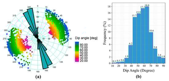
Figure 9.
(a) Steroenet showing the distribution of faults’ dips and orientations identified, along with the entire seismic survey in the Kadanwari field, MIB, Pakistan; (b) a histogram showing the dip angles of the interpreted faults along with their frequency.
4.3. Three-Dimensional Structural Models (3D SMs)
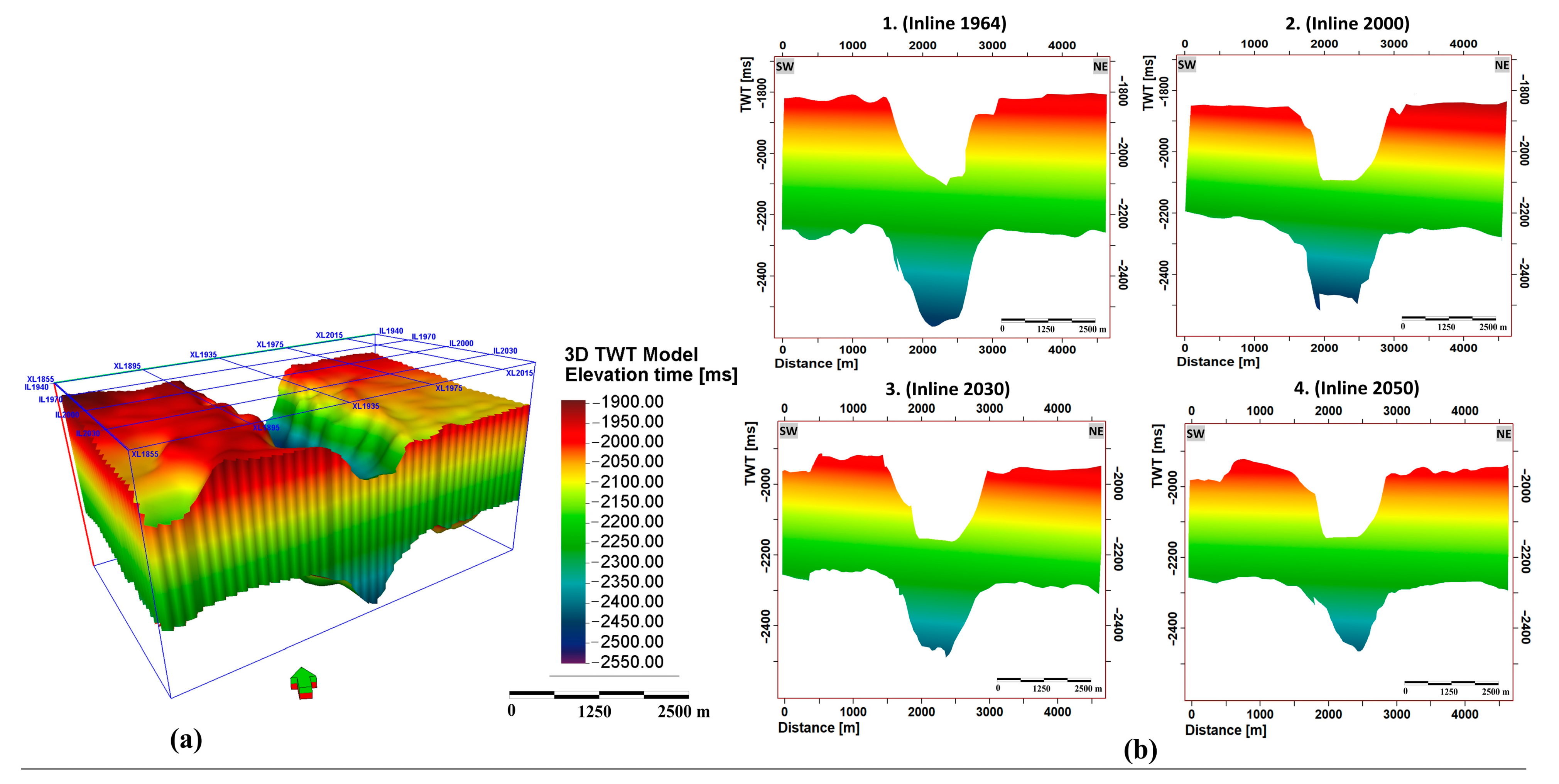
The 3D SMs and several 2D time-domain structural cross-sections have been derived to illustrate the detailed structural and stratigraphic setting of the sequence in the study area. Figure 10a displays the southwestern and southeastern transects of the 3D TWT model, while Figure 10b represents the 2D TWT cross-sections derived from the 3D TWT model result. Figure 11a displays the southwestern and southeastern transect of the 3D SMs derived from VBM. Moreover, the fault system is incorporated into the 2D cross-sections during model computation to constrain the horizons at each fault offset (Figure 11b).

Figure 10.
TWT domain structural model of the early Cretaceous stratigraphic sequence (e.g., G sand interval, E sand interval, and the Sembar Formation): (a) SW–SE view; (b) extracted inline 2D TWT cross-sections.

Figure 11.
Final result of the 3D SM: (a) SW–SE view and (b) SW–NE oriented 2D cross-sections drawn from the 3D SM results.
Detailed structural analysis reveals that the geological structural complexity is a consequence of different tectonic phases of deformation (e.g., extensional and strike-slip deformation from the early Cretaceous to Quaternary). The complex structural mechanics of both extensional and strike-slip movements have been observed in the 3D SMs. These complex structural mechanics were controlled by the normal fault system’s NW–SE dipping. The above-explained normal fault patterns (e.g., negative flower structure) show brittle deformation features, where the interpreted sequences have been displaced relative to each other (amount of displacement) (Figure 11b). These significantly control the structural domains, consisting mainly of half-graben, horst, half-graben, graben, half-graben, and horst, from SW to NE. The thickness of the sequence increases towards the NE. The thickness decreases in the central portion of the region from the top E sand interval to the top Sembar Formation. The hydrocarbon migration direction can be determined from the spatial distribution and composition of the fault system within the early Cretaceous sequences. The geometrical trend of these fault systems creates a pathway that is crucial for hydrocarbon migration in the vertical direction. This up-dip migration of the hydrocarbons from the Sembar formation towards the G and E sand intervals has resulted in hydrocarbon accumulation, validated through seismic attribute analysis and petrophysical modeling.
4.4. Seismic Attributes Interpretation
4.4.1. Variance Edge Attribute
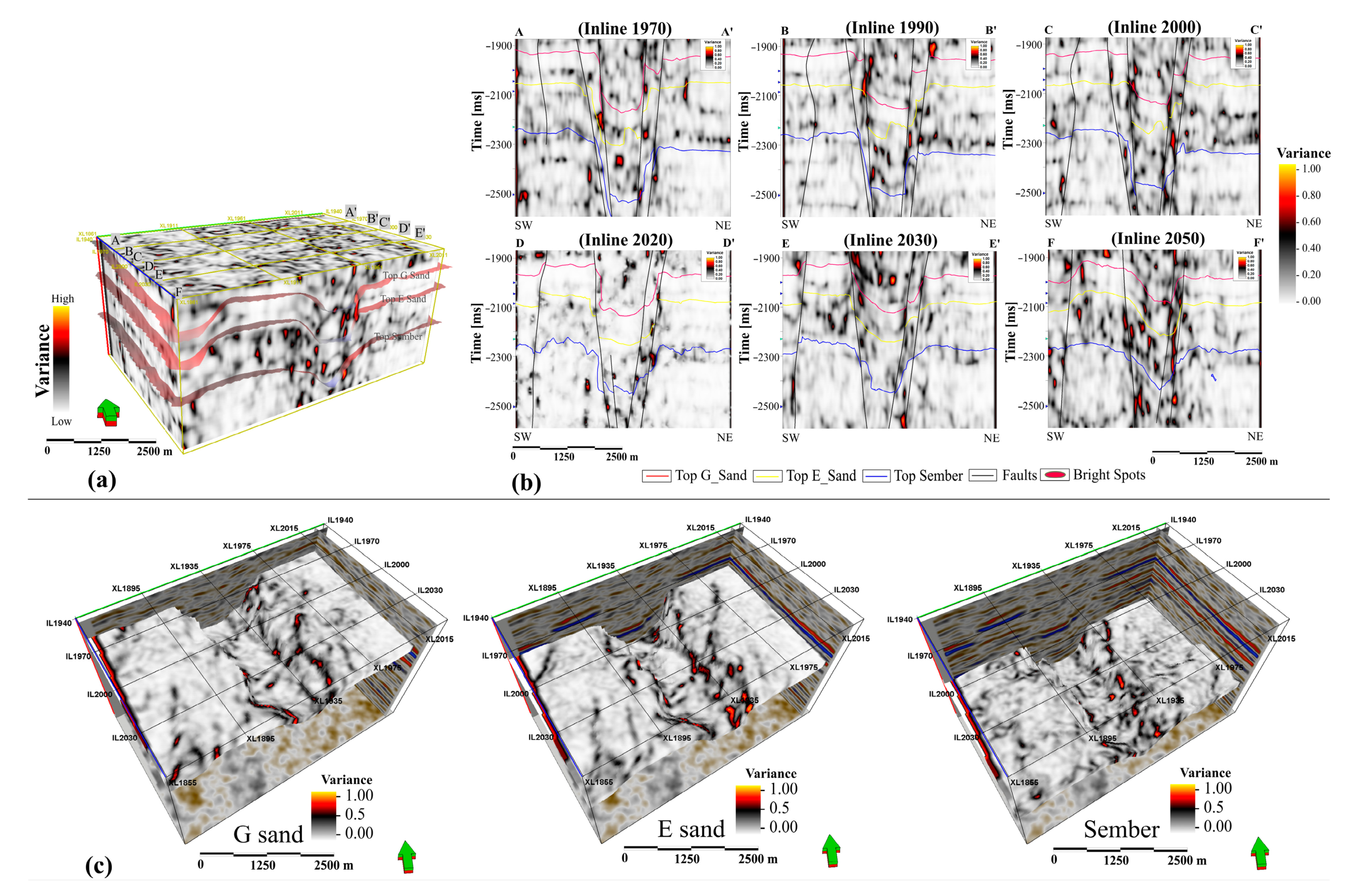
The variance edge attribute indicates discontinuities related to faulting or stratigraphy in the vertical seismic cross-sections and is proved to help depict significant fault zones and fractures, thereby validating fault interpretation. Figure 12 shows the results of the variance edge attribute calculated from the 3D seismic volume, appropriate cross-sections (e.g., A–A′, B–B′, C–C′, D–D′, E–E′ and F–F′), and horizon slices. The horizon slices include the G sand interval, the E sand interval, and the Sembar Formation. The variance edge attribute values in the 2D variance cross-sections and horizon slices range from 0.0 to 1.0. A variance value equal to 1 indicates discontinuity (fault), while a value of 0 variances represents continuous seismic events. The darkest regions (e.g., values ranging from 0.8 to 1) in vertical strips can be interpreted as faults or fractures (Figure 12c). These faults and fractures create an essential pathway for vertical hydrocarbon migration.
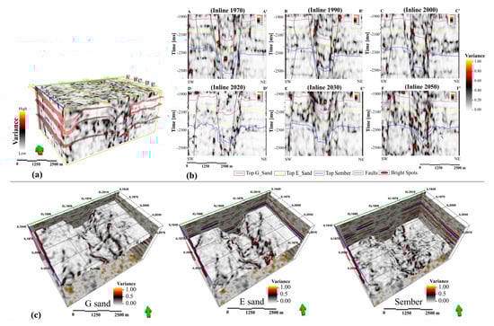
Figure 12.
(a) 3D variance edge attribute volume, (b) 2D extracted variance cross-sections, and (c) 3D variance horizon slices of the G sand interval, the E sand interval, and the Sembar Formation showing discontinuities.
4.4.2. Sweetness Attribute
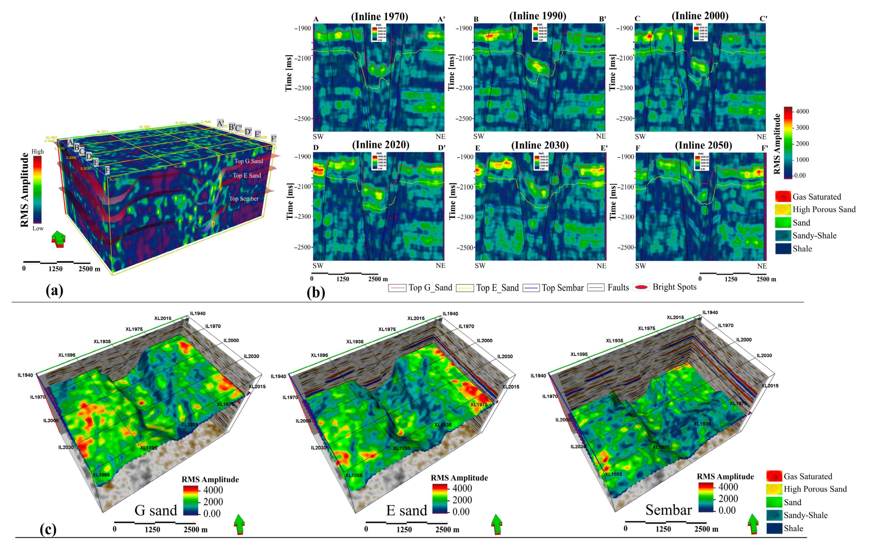
Figure 13 shows the sweetness attribute computed from the 3D seismic volume, corresponding cross-sections (e.g., A–A′, B–B′, C–C′, D–D′, E–E′ and F–F′), and sweetness horizon slices. The high sweetness anomalies (at −1900 to −2300 ms) on the 2D sweetness cross-sections (Figure 13b) and the 3D horizon slices (e.g., G sand and E sand intervals) (Figure 13c) contributed to the high amplitude and low frequency. In contrast, the low sweetness anomalies (at −2300 to −2500 ms) on the 2D sweetness cross-sections and the SW—NE parts of the 3D horizon slices (e.g., the Sembar Formation) due to the seismic reflection low amplitude and high frequency. The high amplitude (high acoustic impedance as opposed to shale) and low-frequency anomalies on the 2D sweetness cross-sections and the 3D sweetness horizon slices represent cleaner and more payable sand zones. These sweet spots suggest the presence of a high proportion of porous sand and seem to hold potential for producing gas in the SW and NE parts of the G and E sand reservoir intervals (Figure 13c). In contrast, areas with low amplitude and high-frequency anomalies within the −2100 to −2300 (ms) in the 2D sweetness cross-sections non-reservoir window (e.g., the Sembar Formation) are shale-prone; the sands here may be interbedded with shale. Although the sweetness attribute effectively distinguishes sand bodies from shale, it does so via the high acoustic impedance contrast between sand and shale.
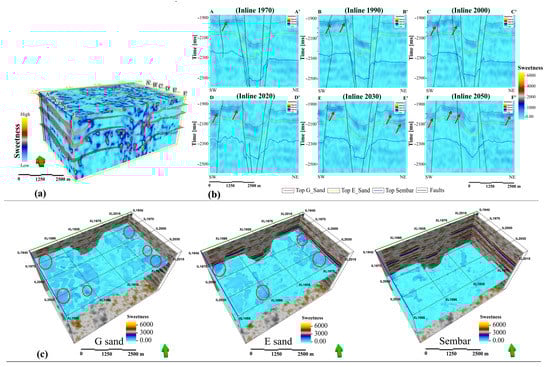
Figure 13.
(a) 3D sweetness attribute volume, (b) 2D extracted sweetness cross-sections, and (c) 3D sweetness horizon slices of the G sand interval, the E sand interval, and the Sembar Formation.
4.4.3. RMS Amplitude Attribute
Figure 14 shows the results of RMS amplitude inferred from the 3D seismic volume, appropriate 2D cross-sections (e.g., A–A′, B–B′, C–C′, D–D′, E–E′ and F–F′), and 3D horizon slices (e.g., G sand interval, E sand interval, and the Sembar Formation). The extracted 2D RMS amplitude cross-section anomalies range from 0 to 4000 ms. These amplitude variations evaluated the structure’s influence on depositional facies. The moderate to high-amplitude anomalies, e.g., between 2500 and 4000 (ms), are often associated with channel sand bodies, high porosity (porous sands), and sand-rich sand shoreward facies, especially gas saturated sand zones. The lateral and horizontal spatial distributions of facies show that faults and fractures significantly reduce the reservoir quality (G and E sand intervals). The gas-saturated sand in the SW and NE parts have high reflectivity, indicating high porosity within the G and E sand intervals (Figure 14c). These sand-rich gas-saturated zones can be considered for future gas exploration in the study area. In comparison, low amplitude anomalies, e.g., between 0 and 2000 (ms), may indicate that these zones contain sandy shale, making them unfavorable for gas production. Such unfavorable zones mainly include the Cretaceous organic-rich shales of the Sembar Formation (Figure 14c).

Figure 14.
(a) 3D RMS amplitude volume, (b) corresponding 2D extracted cross-sections, and (c) 3D RMS amplitude horizon slices of G sand, E sand, and the Sembar Formation.
4.5. Petrophysical Modeling
Petrophysical modeling unveils the reservoir traits and offers suggestions of hydrocarbon-bearing zones. The average petrophysical properties such as Vshale, ∅avg, ∅eff, and SW of the G sand interval in both wells are 36.11%, 12.5%, 7.5%, and 45%, respectively (Table 3). Similarly, the derived average petrophysical properties for the E sand interval in both wells are 30.5%, 17.4%, 12.2%, and 33.2%, respectively (Table 4). A graphical representation of these properties is presented in Figure 15. The overall description of the G and E sand reservoir intervals depends on these petrophysical properties. This may significantly influence the decision-making process in all phases of the planning and executing hydrocarbon activities in the Kadanwari field, MIIB, Pakistan.
Table 3.
Petrophysical properties of the Cretaceous G sand interval in the Kadanwari-10 and Kadanwari-11 wells.
Table 4.
Petrophysical properties of the Cretaceous E sand interval in the Kadanwari-10 and Kadanwari-11 wells.
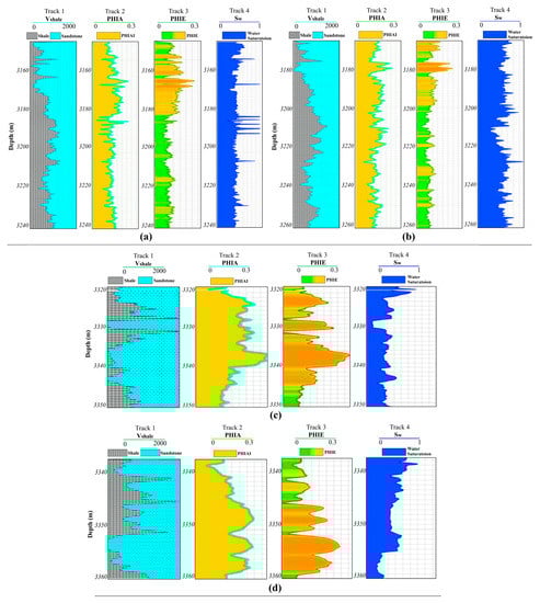
Figure 15.
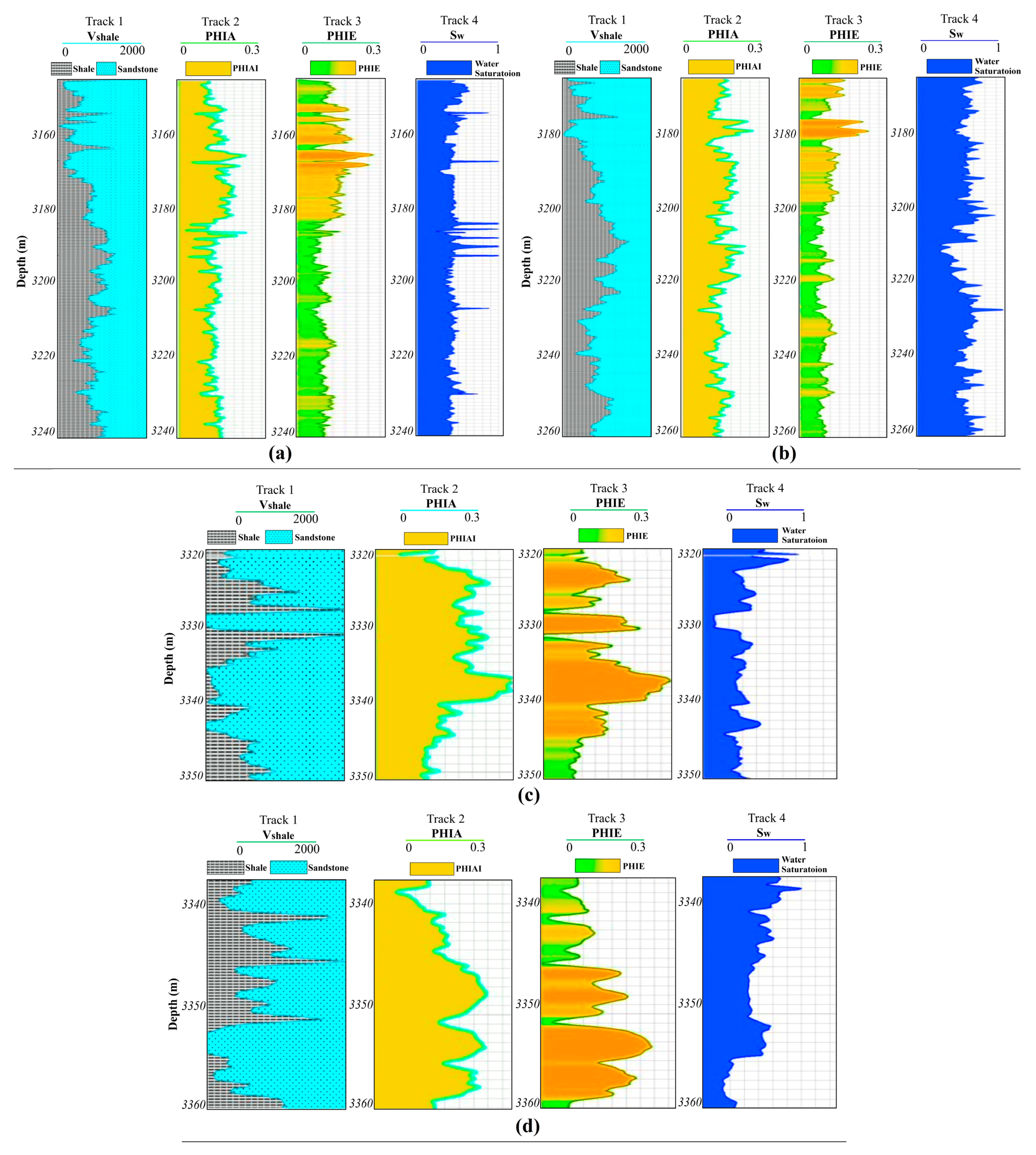
Relationship between the Vshale and volume of sand (track 1), distribution of ∅avg (track 2), distribution of ∅eff (track 3), and the relationship between SW and Shc with respect to the depth at the G sand interval in (a) Kadanwari 10 and (b) Kadanwari-11 wells, and at the E sand interval in (c) Kadanwari 10 and (d) Kadanwari-11 wells.
The GR log response is sensitive to the radioactive emissions predominantly concentrated in the clay minerals of shale and clean sand (feldspar-rich) [43]. The GR response in track 1 of each understudy well confirms the reservoir lithology to be sandstone (Figure 15a). Figure 15a represents the relationship between Vshale and sand content (track 1), ∅avg distribution (track 2), ∅eff distribution (track 3), and the relation between SW and Shc (track 4) at the G sand interval in the Kadanwari-10 and 11 wells. Similarly, Figure 15b represents the relationship between Vshale and sand content (track 1), ∅avg distribution (track 2), ∅eff distribution (track 3), and the relation between SW and Shc (track 4) at the E sand interval in the Kadanwari-10 and 11 wells.
5. Discussion
5.1. Integration of 3D SM and JGC for Hydrocarbon Evaluation
Knowledge of structural, lithological, and petrophysical characteristics is essential to reducing the uncertainties associated with reservoir description. Herein, 3D seismic data and well logs data have been critically analyzed to evaluate the complex and heterogeneous depositional environment of the early Cretaceous stratigraphic sequence, along with structural and stratigraphic characteristics, distribution of associated petrophysical properties, and spatial facies for reliable reservoir characterization. The result indicates that the early Cretaceous stratigraphic sequence appears irregularly, with faulted structural highs bounded by extension-related normal faults, heterogeneous nature of reservoir intervals, and potential gas-saturated zones.
The structural interpretation of the early Cretaceous stratigraphic sequence indicates that the interpreted horizons (e.g., G sand, E sand, and the Sembar Formation) appear normal faulted extension-related horsts, half-graben, and graben structures (Figure 11). The normal faulted inversion-related horsts, half-graben, and graben structures show how the sedimentary layer’s structural features have contributed to the formation of traps and conduit mechanisms. In general, due to the exact kinematic mechanisms involved in the sequential deformation of the Kadanwari field, the structural deformation of each horizon is equal in orientation and extent (Figure 11b). However, the E sand interval seems to be more deformed than the G sand interval and the Sembar Formation. The geometric tendency of the extension-related normal fault in the early Cretaceous stratigraphic sequence is essential because it has created channels for hydrocarbon migration in the vertical direction. Hydrocarbon enrichment in the G and E sand reservoir intervals was positively related to the complexity of the internal structure of normal faults. The hydrocarbon concentration and dominance of these normal faults are more intense towards the central part of the seismic volume, where the faults are closely spaced. The normal fault plane profiles show the hanging wall and footwall cutoffs (Figure 11b). These profiles are useful for understanding the seal behavior for hydrocarbon potential and prospect evaluation.
Using 3D SM, we determined that the extension–related normal faults’ geometrical trend created an essential pathway for the up-dip migration of hydrocarbons from the source rock (the Sembar Formation) towards the G and E sand reservoir intervals, resulting in hydrocarbon accumulation. These statements are validated here, as the moderate to high RMS amplitude anomalies are often associated with gas–saturated sand zones (Figure 14c). The hydrocarbon prospects have high reflectivity, indicating high porosity, which can be seen on both the sweetness (Figure 13b) and RMS amplitude (Figure 14b) attributes within the G and E sand intervals. In addition, the RMS amplitude attribute is advantageous compared with the sweetness attribute because the RMS amplitude attribute has a higher resolution when depicting the porous zones and DHIs. These results can significantly reduce the risk associated with hydrocarbon exploration and development in the Kadanwari field, MIB.
The calculated values of the Shc form the basis of future production forecasts and the determination of the economic viability of a discovered reservoir. Therefore, high accuracy is needed when determining SW, as it is used to calculate the estimated Shc reserves. The low values found for Vshale content in the Kadanwari 10 and 11 wells indicate the cleanliness of the sandstone. Accordingly, the shale and sandstone facies were separated by a 40% cutoff value in the targeted reservoir intervals, i.e., G and E sands. The Vshale contents in the G and E sand intervals are influenced by clay minerals, which reduce the ∅avg and ∅eff. The high values of ∅eff refer to better volume estimation, and thus, a theoretically good reservoir, and vice versa. These high values of ∅eff indicate the amounts of connected pore spaces in the reservoir intervals [43]. The G and E sand reservoir interval properties, as derived from our petrophysical modeling, are in good agreement with the results of the regional study conducted by [40,43].
5.2. Analysis of Gas Reserve of the Kadanwari Field
Graphical representations of the Shc at the G and E sand reservoir intervals are presented in track 4 in Figure 15. The petrophysical modeling results show that these intervals have good Shc, as the SW is below 60% (Table 5). A comparison between the G and E sand interval petrophysical properties shows that the E sand interval has good ∅eff and Shc, with an apparent gas effect revealed by the cross-overs of the DT and NPHI logs curves (Figure 6). Therefore, it can be considered as an economically viable reservoir interval. The Shc percentage of the E sand interval is satisfactory for exploration purposes.
Table 5.
Depth range, thickness, and Shc (%) of the Cretaceous G and E sand intervals in Kadanwari-10 and 11 wells.
The annual report (2010–2011) of petroleum exploration and production activities in Pakistan analyzed the reserves of the Kadanwari field (Table 6) [7]. The Kadanwari field exhibits a significant amount of original recoverable gas reserves, i.e., 1110 billion cubic feet (Bcf) equivalent to 190 million barrels of oil equivalent (Mboe), respectively. From these original recoverable gas reserves, 420 (Bcf) has been extracted from the Kadanwari field. As of 30 June 2011, the balance recoverable gas reserves were 690 Bcf, equivalent to 110 Mboe. The collective original recoverable reserves of the Kadanwari field—280 Mboe—are now limited to 129 Mboe [7]. Thus, many hydrocarbon reserves are present in the Kadanwari field. The high level of gas reserves in the Kadanwari field compared to other fields (such as the Miano field) may be attributed to its complex structural configuration (e.g., negative flower structure of fault system), reservoir compartmentalization, and the up-dip migration of the hydrocarbons into the reservoir intervals (e.g., G and E sands).
Table 6.
The gas reserves of the Kadanwari and Miano fields as of 30 June 2011.
5.3. Comparative Analysis with Other Reservoirs
The detailed structural interpretation of the 3D SMs and appropriate 2D cross-sections has revealed that the geological structural complexity is a consequence of different tectonic phases of deformation (compressional regimes of the surrounding plate boundary). The structural and stratigraphic characteristics results derived from the 3D FSMs, the 3D TWT model, the 3D SMs, the dip angle models, the rose diagram, and the histogram agree with the regional studies conducted by other researchers [7,45,49]. These studies show similar structural and stratigraphic characteristics and patterns. According to [7], most faults dip towards the southwest, with an average throw in the order of about 50 m and a maximum throw of 113 m in the Kadanwari area. Wrench or strike-slip faults are absent, except for one potential one wrench fault (F3) to the south in the Kadanwari field (Figure 9a). Based on this, the possibility of strike-slip deformation may also be inferred. References [7,45,49] also stressed that the Kadanwari field is structurally essential due to the presence of fault-bounded structures, which may be considered as potential prospects. The structural characteristics of the nearby fields within the MIB and LIB, such as the Miano, Sawan, and Zamzama fields, can also be correlated with the conducted study of the Kadanwari field.
The adopted methods of 3D SM and JGC can also be utilized in the international basins having the same geology of extensional regimes featuring the horst and graben structures as a petroleum play. These include the Bach Ho oilfield in Cuu Long Basin of Vietnam [61] and the Mannar frontier sedimentary basin of Sri Lanka [62]. In addition, this study is helpful to characterize and evaluate reservoir geometrical characteristics, facies, and properties to reduce uncertainties and improve the success rate of future exploration and development plans pertaining to hydrocarbons in the regions having the same geology globally. In general, conventional methods remain inadequate in individual or integrated form. Therefore, machine learning tools may provide guidance for detailed structural and petrophysical evaluation. In future work, the manual structural interpretation, seismic attributes maps, and petrophysical properties can be used as input databases of machine learning, especially deep learning, models for subsequent automated 3D structural, facies, and petrophysical modeling.
6. Conclusions
We introduced a novel methodology of 3D structural modeling (3D SM) and joint geophysical characterization (JGC), which comprises seismic interpretation-aided 3D structural modeling, seismic attributes, and petrophysical modeling for reservoir characterization in the Kadanwari field, Middle Indus Basin (MIB), Pakistan. Our main findings are as follow:
- (1)
- The 3D structural interpretation illustrates the complex structural mechanics, controlled by the NW–SE dipping normal faults system, operating in the early Cretaceous stratigraphic sequence. The identified features include horsts, half-graben, and graben structures. The spatial distribution of the fault system shows that the overall pattern of the interpreted fault system can be regarded as a negative flower structure. The negative flower structure incorporates the combined effects of extensional and strike-slip motion in the study area. In general, the horsts, half-graben, and graben, along with the faults, have geometrically determined reservoir (G and E sand intervals) geomorphology, up-dip hydrocarbon migration, the development of the local strata, the distribution of facies and properties, and internal structural deformation;
- (2)
- The variance edge attribute enhanced the geometric distribution of the faults within the seismic data. The sweetness attribute distinguished the sand facies from shale, as the increased amplitude and lower frequency content represent cleaner and more payable sand zones. In contrast, areas with low amplitude and high-frequency anomalies are susceptible to shale. The RMS amplitude and sweetness attribute results indicate the hydrocarbon zones. Relatively high RMS amplitude attribute values are usually connected with lithological changes, sand-rich shoreward facies, bright spots, and especially gas-saturated sand zones. In comparison, low amplitudes anomalies indicate the zones of sandy-shale, shale, and pro-delta facies;
- (3)
- Petrophysical modeling reveals the important parameters of G and E sand reservoir intervals. The ∅avg values calculated via the Sonic–Raymer (SR) porosity model, the RHOB log, and the NPHI log show that the G and E sand reservoir intervals have good porosities. Moreover, the E sand interval has good ∅eff and Shc and displays clear signs of gas effects verified by the cross-overs of density and neutron log curves. Therefore, it can be considered an economically viable reservoir interval for future hydrocarbon production.
Author Contributions
Conceptualization, U.K. and B.Z.; methodology, U.K. and J.D.; software, U.K.; validation, B.Z., J.D., and M.K.; formal analysis, Y.T. and S.A.; investigation, I.A.; data curation, S.H.; writing—original draft preparation, U.K. and Z.J.; writing—review and editing, Y.T. and U.K.; funding acquisition, B.Z. All authors have read and agreed to the published version of the manuscript.
Funding
This study was supported by grants from the National Natural Science Foundation of China (Grant No. 42072326 and 41772348) and the National Key Research and Development Program of China (Grant No. 2019YFC1805905).
Data Availability Statement
The dataset of the current study are not publicaly availible due to a data privacy agreement we signed with the Directorate General of Petroleum Concessions (DGPC), Pakistan, but are availible from the corresponding author on reasonable request.
Acknowledgments
The authors thank Landmark Resources (LMKR) and the Directorate General of Petroleum Concessions (DGPC), Pakistan, for providing the dataset. Many thanks to Umar Ashraf (Yunnan University, China) for revising the final version of this manuscript.
Conflicts of Interest
The authors declare no conflict of interest.
References
- Qadri, S.T.; Islam, M.A.; Shalaby, M.R.; Ali, S.H. Integration of 1D and 3D modeling schemes to establish the Farewell Formation as a self-sourced reservoir in Kupe Field, Taranaki Basin, New Zealand. Front. Earth Sci. 2020, 15, 631–648. [Google Scholar] [CrossRef]
- Thota, S.T.; Islam, M.A.; Shalaby, M.R. A 3D geological model of a structurally complex relationships of sedimentary Facies and Petrophysical Parameters for the late Miocene Mount Messenger Formation in the Kaimiro-Ngatoro field, Taranaki Basin, New Zealand. J. Pet. Explor. Prod. Technol. 2021, 11, 1–36. [Google Scholar] [CrossRef]
- Masters, C.D.; Root, D.H.; Attanasi, E.D.; Tedeschi, M.; Singh, S.; du Plessis, M.; Wong, S.; Redford, D.; Wightman, D.; MacGillivray, J. World resources of crude oil and natural gas. Energy Explor. Exploit. 1991, 9, 354–374. [Google Scholar]
- Mangi, H.N.; Chi, R.; DeTian, Y.; Sindhu, L.; He, D.; Ashraf, U.; Fu, H.; Zixuan, L.; Zhou, W.; Anees, A. The ungrind and grinded effects on the pore geometry and adsorption mechanism of the coal particles. J. Nat. Gas Sci. Eng. 2022, 100, 104463. [Google Scholar] [CrossRef]
- Mangi, H.N.; Detian, Y.; Hameed, N.; Ashraf, U.; Rajper, R.H. Pore structure characteristics and fractal dimension analysis of low rank coal in the Lower Indus Basin, SE Pakistan. J. Nat. Gas Sci. Eng. 2020, 77, 103231. [Google Scholar] [CrossRef]
- Sheikh, N.; Giao, P.H. Evaluation of shale gas potential in the lower cretaceous Sembar formation, the southern Indus basin, Pakistan. J. Nat. Gas Sci. Eng. 2017, 44, 162–176. [Google Scholar] [CrossRef]
- Saif-Ur-Rehman, K.J.; Lin, D.; Ehsan, S.A.; Jadoon, I.A.; Idrees, M. Structural styles, hydrocarbon prospects, and potential of Miano and Kadanwari fields, Central Indus Basin, Pakistan. Arab. J. Geosci. 2020, 13, 97. [Google Scholar]
- Ahmad, N.; Khan, S.; Al-Shuhail, A. Seismic Data Interpretation and Petrophysical Analysis of Kabirwala Area Tola (01) Well, Central Indus Basin, Pakistan. Appl. Sci. 2021, 11, 2911. [Google Scholar] [CrossRef]
- Khan, U.; Zhang, B.; Du, J.; Jiang, Z. 3D structural modeling integrated with seismic attribute and petrophysical evaluation for hydrocarbon prospecting at the Dhulian Oilfield, Pakistan. Front. Earth Sci. 2021, 15, 649–675. [Google Scholar] [CrossRef]
- Bodunde, S.; Enikanselu, P. Integration of 3D-seismic and petrophysical analysis with rock physics analysis in the characterization of SOKAB field, Niger delta, Nigeria. J. Pet. Explor. Prod. Technol. 2019, 9, 899–909. [Google Scholar] [CrossRef] [Green Version]
- Hossain, M.I.S.; Woobaidullah, A.; Rahman, M.J. Reservoir characterization and identification of new prospect in Srikail gas field using wireline and seismic data. J. Pet. Explor. Prod. Technol. 2021, 11, 2481–2495. [Google Scholar] [CrossRef]
- Kargarpour, M.A. Carbonate reservoir characterization: An integrated approach. J. Pet. Explor. Prod. Technol. 2020, 10, 2655–2667. [Google Scholar] [CrossRef]
- Islam, M.A.; Yunsi, M.; Qadri, S.T.; Shalaby, M.R.; Haque, A.E. Three-dimensional structural and petrophysical modeling for reservoir characterization of the Mangahewa formation, Pohokura Gas-Condensate Field, Taranaki Basin, New Zealand. Nat. Resour. Res. 2021, 30, 371–394. [Google Scholar] [CrossRef]
- Li, X.; Zhou, N.; Xie, X. Reservoir characteristics and three-dimensional architectural structure of a complex fault-block reservoir, beach area, China. J. Pet. Explor. Prod. Technol. 2018, 8, 1535–1545. [Google Scholar] [CrossRef] [Green Version]
- Osinowo, O.O.; Ayorinde, J.O.; Nwankwo, C.P.; Ekeng, O.; Taiwo, O. Reservoir description and characterization of Eni field Offshore Niger Delta, southern Nigeria. J. Pet. Explor. Prod. Technol. 2018, 8, 381–397. [Google Scholar] [CrossRef] [Green Version]
- Haque, A.E.; Islam, M.A.; Shalaby, M.R. Structural modeling of the Maui gas field, Taranaki basin, New Zealand. Pet. Explor. Dev. 2016, 43, 965–975. [Google Scholar] [CrossRef]
- Mutebi, S.; Sen, S.; Sserubiri, T.; Rudra, A.; Ganguli, S.S.; Radwan, A.E. Geological characterization of the Miocene–Pliocene succession in the Semliki Basin, Uganda: Implications for hydrocarbon exploration and drilling in the East African Rift System. Nat. Resour. Res. 2021, 30, 4329–4354. [Google Scholar] [CrossRef]
- Abdeen, M.M.; Ramadan, F.S.; Nabawy, B.S.; El Saadawy, O. Subsurface Structural Setting and Hydrocarbon Potentiality of the Komombo and Nuqra Basins, South Egypt: A Seismic and Petrophysical Integrated Study. Nat. Resour. Res. 2021, 30, 3575–3603. [Google Scholar] [CrossRef]
- Ashraf, U.; Zhu, P.; Yasin, Q.; Anees, A.; Imraz, M.; Mangi, H.N.; Shakeel, S. Classification of reservoir facies using well log and 3D seismic attributes for prospect evaluation and field development: A case study of Sawan gas field, Pakistan. J. Pet. Sci. Eng. 2019, 175, 338–351. [Google Scholar] [CrossRef]
- Hussain, M.; Ahmed, N.; Chun, W.Y.; Khalid, P.; Mahmood, A.; Ahmad, S.R.; Rasool, U. Reservoir characterization of basal sand zone of lower Goru Formation by petrophysical studies of geophysical logs. J. Geol. Soc. India 2017, 89, 331–338. [Google Scholar] [CrossRef]
- Moore, G.F. 3-D seismic interpretation. Am. Geophys. Union 2009, 90, 161. [Google Scholar] [CrossRef] [Green Version]
- Vo Thanh, H.; Sugai, Y.; Sasaki, K. Impact of a new geological modelling method on the enhancement of the CO2 storage assessment of E sequence of Nam Vang field, offshore Vietnam. Energy Sources Part A Recovery Util. Environ. Eff. 2020, 42, 1499–1512. [Google Scholar] [CrossRef]
- Houlding, S. 3D Geoscience Modeling: Computer Techniques for Geological Characterization; Springer Science & Business Media: Berlin/Heidelberg, Germany, 2012. [Google Scholar]
- Lajaunie, C.; Courrioux, G.; Manuel, L. Foliation fields and 3D cartography in geology: Principles of a method based on potential interpolation. Math. Geol. 1997, 29, 571–584. [Google Scholar] [CrossRef]
- Mallet, J.-L. Geomodeling; Oxford University Press: Oxford, UK, 2002. [Google Scholar]
- Wu, Q.; Xu, H.; Zou, X. An effective method for 3D geological modeling with multi-source data integration. Comput. Geosci. 2005, 31, 35–43. [Google Scholar] [CrossRef]
- Zhang, B.; Chen, Y.; Huang, A.; Lu, H.; Cheng, Q. Geochemical field and its roles on the 3D prediction fo concealed ore-bodies. Acta Petrol. Sin. 2018, 34, 352–362. [Google Scholar]
- Wang, L.; Wu, X.; Zhang, B.; Li, X.; Huang, A.; Meng, F.; Dai, P. Recognition of significant surface soil geochemical anomalies via weighted 3D shortest-distance field of subsurface orebodies: A case study in the Hongtoushan copper mine, NE China. Nat. Resour. Res. 2019, 28, 587–607. [Google Scholar] [CrossRef]
- Thanh, H.V.; Sugai, Y.; Nguele, R.; Sasaki, K. Integrated workflow in 3D geological model construction for evaluation of CO2 storage capacity of a fractured basement reservoir in Cuu Long Basin, Vietnam. Int. J. Greenh. Gas Control 2019, 90, 102826. [Google Scholar] [CrossRef]
- Adelu, A.O.; Aderemi, A.; Akanji, A.O.; Sanuade, O.A.; Kaka, S.I.; Afolabi, O.; Olugbemiga, S.; Oke, R. Application of 3D static modeling for optimal reservoir characterization. J. Afr. Earth Sci. 2019, 152, 184–196. [Google Scholar] [CrossRef]
- Ayodele, O.L.; Chatterjee, T.; Opuwari, M. Static reservoir modeling using stochastic method: A case study of the cretaceous sequence of Gamtoos Basin, Offshore, South Africa. J. Pet. Explor. Prod. Technol. 2021, 11, 4185–4200. [Google Scholar] [CrossRef]
- Jung, A.; Aigner, T.; Palermo, D.; Nardon, S.; Pontiggia, M. A Hierarchical Database on Carbonate Geobodies and Its Application to Reservoir Modelling Using Multi-Point Statistics. In Proceedings of the 72nd EAGE Conference and Exhibition Incorporating SPE EUROPEC 2010, Barcelona, Spain, 14–17 June 2010; p. cp-161-00314. [Google Scholar]
- Li, J.; Zhang, X.; Lu, B.; Ahmed, R.; Zhang, Q. Static Geological Modelling with Knowledge Driven Methodology. Energies 2019, 12, 3802. [Google Scholar] [CrossRef] [Green Version]
- Okoli, A.E.; Agbasi, O.E.; Lashin, A.A.; Sen, S. Static Reservoir Modeling of the Eocene Clastic Reservoirs in the Q-Field, Niger Delta, Nigeria. Nat. Resour. Res. 2021, 30, 1411–1425. [Google Scholar] [CrossRef]
- Thanh, H.V.; Sugai, Y. Integrated modelling framework for enhancement history matching in fluvial channel sandstone reservoirs. Upstream Oil Gas Technol. 2021, 6, 100027. [Google Scholar] [CrossRef]
- Vo Thanh, H.; Lee, K.-K. 3D geo-cellular modeling for Oligocene reservoirs: A marginal field in offshore Vietnam. J. Pet. Explor. Prod. Technol. 2022, 12, 1–19. [Google Scholar] [CrossRef]
- Ali, M.; Abdelhady, A.; Abdelmaksoud, A.; Darwish, M.; Essa, M.A. 3D static modeling and petrographic aspects of the Albian/Cenomanian Reservoir, Komombo Basin, Upper Egypt. Nat. Resour. Res. 2020, 29, 1259–1281. [Google Scholar] [CrossRef]
- Azeem, T.; Yanchun, W.; Khalid, P.; Xueqing, L.; Yuan, F.; Lifang, C. An application of seismic attributes analysis for mapping of gas bearing sand zones in the sawan gas field, Pakistan. Acta Geod. Geophys. 2016, 51, 723–744. [Google Scholar] [CrossRef]
- Naseer, M.T. Seismic attributes and quantitative stratigraphic simulation’application for imaging the thin-bedded incised valley stratigraphic traps of Cretaceous sedimentary fairway, Pakistan. Mar. Pet. Geol. 2021, 134, 105336. [Google Scholar] [CrossRef]
- Ali, M.; Khan, M.J.; Ali, M.; Iftikhar, S. Petrophysical analysis of well logs for reservoir evaluation: A case study of “Kadanwari” gas field, middle Indus basin, Pakistan. Arab. J. Geosci. 2019, 12, 1–12. [Google Scholar] [CrossRef]
- Raza, M.; Khan, F.; Khan, M.; Riaz, M.; Khan, U. Reservoir characterization of the B-interval of lower goru formation, miano 9 and 10, miano area, Lower Indus Basin, Pakistan. Env. Earth Sci. Res. J. 2020, 7, 18–32. [Google Scholar] [CrossRef]
- Ahmad, N.; Spadini, G.; Palekar, A.; Subhani, M.A. Porosity prediction using 3D seismic inversion Kadanwari gas field, Pakistan. Pak. J. Hydrocarb. Res. 2007, 17, 95–102. [Google Scholar]
- Khan, M.J.; Khan, H.A. Petrophysical logs contribute in appraising productive sands of Lower Goru Formation, Kadanwari concession, Pakistan. J. Pet. Explor. Prod. Technol. 2018, 8, 1089–1098. [Google Scholar] [CrossRef] [Green Version]
- Dar, Q.U.; Pu, R.; Baiyegunhi, C.; Shabeer, G.; Ali, R.I.; Ashraf, U.; Sajid, Z.; Mehmood, M. The impact of diagenesis on the reservoir quality of the early Cretaceous Lower Goru sandstones in the Lower Indus Basin, Pakistan. J. Pet. Explor. Prod. Technol. 2021, 11, 1–16. [Google Scholar] [CrossRef]
- Ahmad, N.; Chaudhry, S. Kadanwari Gas Field, Pakistan: A disappointment turns into an attractive development opportunity. Pet. Geosci. 2002, 8, 307–316. [Google Scholar] [CrossRef]
- Kazmi, A.; Jan, M. Geology and Tectonics of Pakistan; Graphic Publishers: Santa Ana, CA, USA, 1997; p. 554. ISBN 9698375007. [Google Scholar]
- Saif-Ur-Rehman, K.J.; Mehmood, M.F.; Shafiq, Z.; Jadoon, I.A. Structural styles and petroleum potential of Miano block, central Indus Basin, Pakistan. Int. J. Geosci. 2016, 7, 1145. [Google Scholar]
- Ahmad, N.; Fink, P.; Sturrock, S.; Mahmood, T.; Ibrahim, M. Sequence stratigraphy as predictive tool in lower goru fairway, lower and middle Indus platform, Pakistan. PAPG ATC 2004, 1, 85–104. [Google Scholar]
- Ahmed, W.; Azeem, A.; Abid, M.F.; Rasheed, A.; Aziz, K. Mesozoic Structural Architecture of the Middle Indus Basin, Pakistan—Controls and Implications. In Proceedings of the PAPG/SPE Annual Technical Conference, Islamabad, Pakistan, 26 November 2013; pp. 1–13. [Google Scholar]
- Shakir, U.; Ali, A.; Hussain, M.; Azeem, T.; Bashir, L. Selection of Sensitive Post-Stack and Pre-Stack Seismic Inversion Attributes for Improved Characterization of Thin Gas-Bearing Sands. Pure Appl. Geophys. 2021, 179, 169–196. [Google Scholar] [CrossRef]
- Faleide, T.S.; Braathen, A.; Lecomte, I.; Mulrooney, M.J.; Midtkandal, I.; Bugge, A.J.; Planke, S. Impacts of seismic resolution on fault interpretation: Insights from seismic modelling. Tectonophysics 2021, 816, 229008. [Google Scholar] [CrossRef]
- Kim, M.; Yu, J.; Kang, N.-K.; Kim, B.-Y. Improved Workflow for Fault Detection and Extraction Using Seismic Attributes and Orientation Clustering. Appl. Sci. 2021, 11, 8734. [Google Scholar] [CrossRef]
- Khan, M.; Abdelmaksoud, A. Unfolding impacts of freaky tectonics on sedimentary sequences along passive margins: Pioneer findings from western Indian continental margin (Offshore Indus Basin). Mar. Pet. Geol. 2020, 119, 104499. [Google Scholar] [CrossRef]
- Qadri, S.T.; Islam, M.A.; Shalaby, M.R. Three-dimensional petrophysical modelling and volumetric analysis to model the reservoir potential of the Kupe Field, Taranaki Basin, New Zealand. Nat. Resour. Res. 2019, 28, 369–392. [Google Scholar] [CrossRef]
- Taner, M.T.; Koehler, F.; Sheriff, R. Complex seismic trace analysis. Geophysics 1979, 44, 1041–1063. [Google Scholar] [CrossRef]
- Ahmad, M.N.; Rowell, P. Application of spectral decomposition and seismic attributes to understand the structure and distribution of sand reservoirs within Tertiary rift basins of the Gulf of Thailand. Lead. Edge 2012, 31, 630–634. [Google Scholar] [CrossRef]
- Abuamarah, B.A.; Nabawy, B.S.; Shehata, A.M.; Kassem, O.M.; Ghrefat, H. Integrated geological and petrophysical characterization of oligocene deep marine unconventional poor to tight sandstone gas reservoir. Mar. Pet. Geol. 2019, 109, 868–885. [Google Scholar] [CrossRef]
- Iqbal, M.A.; Rezaee, R. Porosity and Water Saturation Estimation for Shale Reservoirs: An Example from Goldwyer Formation Shale, Canning Basin, Western Australia. Energies 2020, 13, 6294. [Google Scholar] [CrossRef]
- Dolan, P. Pakistan: A history of petroleum exploration and future potential. Geol. Soc. Lond. Spec. Publ. 1990, 50, 503–524. [Google Scholar] [CrossRef]
- Sam-Marcus, J.; Enaworu, E.; Rotimi, O.J.; Seteyeobot, I. A proposed solution to the determination of water saturation: Using a modelled equation. J. Pet. Explor. Prod. Technol. 2018, 8, 1009–1015. [Google Scholar] [CrossRef] [Green Version]
- Cuong, T.X.; Warren, J. Bach ho field, a fractured granitic basement reservoir, Cuu Long Basin, offshore SE Vietnam: A “buried-hill” play. J. Pet. Geol. 2009, 32, 129–156. [Google Scholar] [CrossRef]
- Kularathna, E.; Pitawala, H.; Senaratne, A.; Ratnayake, A. Play distribution and the hydrocarbon potential of the Mannar Basin, Sri Lanka. J. Pet. Explor. Prod. Technol. 2020, 10, 2225–2243. [Google Scholar] [CrossRef]

Publisher’s Note: MDPI stays neutral with regard to jurisdictional claims in published maps and institutional affiliations. |
© 2022 by the authors. Licensee MDPI, Basel, Switzerland. This article is an open access article distributed under the terms and conditions of the Creative Commons Attribution (CC BY) license (https://creativecommons.org/licenses/by/4.0/).