
A Feature-Based Approach for Sentiment Quantification Using Machine Learning

 , and
, and
Abstract
:1. Introduction
- Novel feature sets are proposed such as pos, tweet, specific, content, and sentiment, with the ranking of features carried out using feature selection approaches.
- Deep features including word2vec and GloVe are used for sentiment analysis, and these features are considered for sentiment quantification.
- Machine learning approaches have been investigated, including: (1) traditional techniques—Support Vector Machine (SVM), Naïve Bayes (NB), and Decision Tree (DT); (2) ensemble learners—Random Forest (RF) and AdaBoost; (3) deep learning-based—Deep Belief Network (DBN), Convolutional Neural Network (CNN), and Recurrent Neural Network (RNN).
- The results for sentiment quantification are computed on SemEval2016, SemEval2017, STS-Gold, and Sanders. Standard performance evaluation measures, including Kullback–Leibler divergence (KLD), relative absolute error (RAE), and absolute error (AE), are applied for the evaluation of classifiers.
2. Related Work
2.1. Sentiment Quantification
2.1.1. Aggregated Methods
2.1.2. Non-Aggregated Methods
2.1.3. Ensemble-Based Methods
2.2. Problem Statement and Formulation
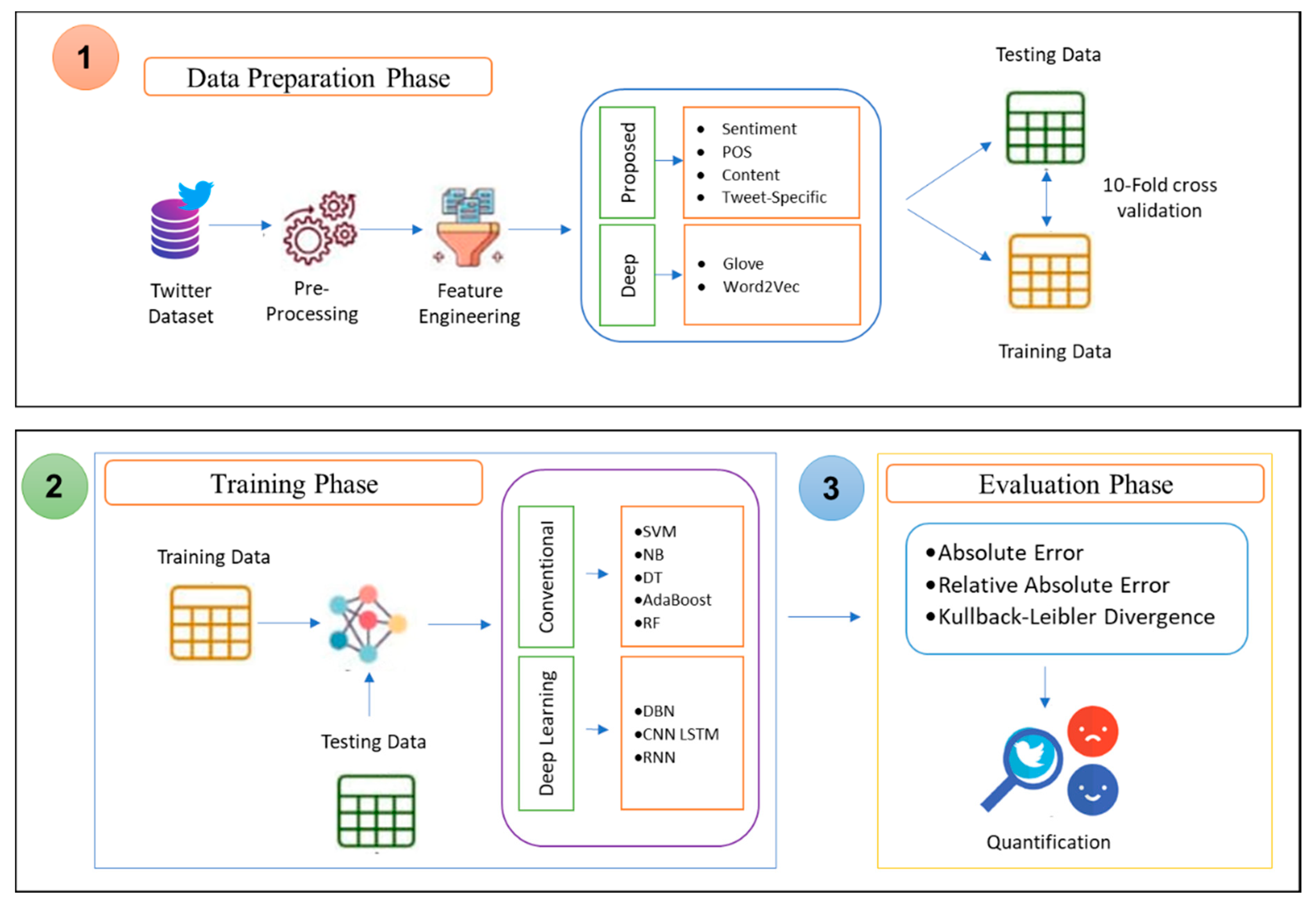
3. Proposed Research Methodology
3.1. Framework for Sentiment Quantification
3.2. Feature Engineering
3.2.1. Proposed Feature Sets
3.2.2. Feature Selection and Ranking
3.3. Classification Algorithms Applied
3.3.1. Machine Learning Techniques
Support Vector Machine (SVM)
Decision Tree (DT)
3.3.2. Ensemble Learning Techniques
AdaBoost
Random Forest (RF)
3.3.3. Deep Learning Techniques
Deep Belief Networks (DBN)
CNN-LSTM
Recurrent Neural Network (RNN)
3.4. Datasets
3.4.1. SemEval2016
3.4.2. SemEval2017
3.4.3. STS-Gold
3.4.4. Sanders
3.5. Performance Evaluation Measures
3.5.1. Absolute Error (AE)
3.5.2. Relative Absolute Error (RAE)
3.5.3. Kullback–Leibler Divergence (KLD)
4. Results and Discussion
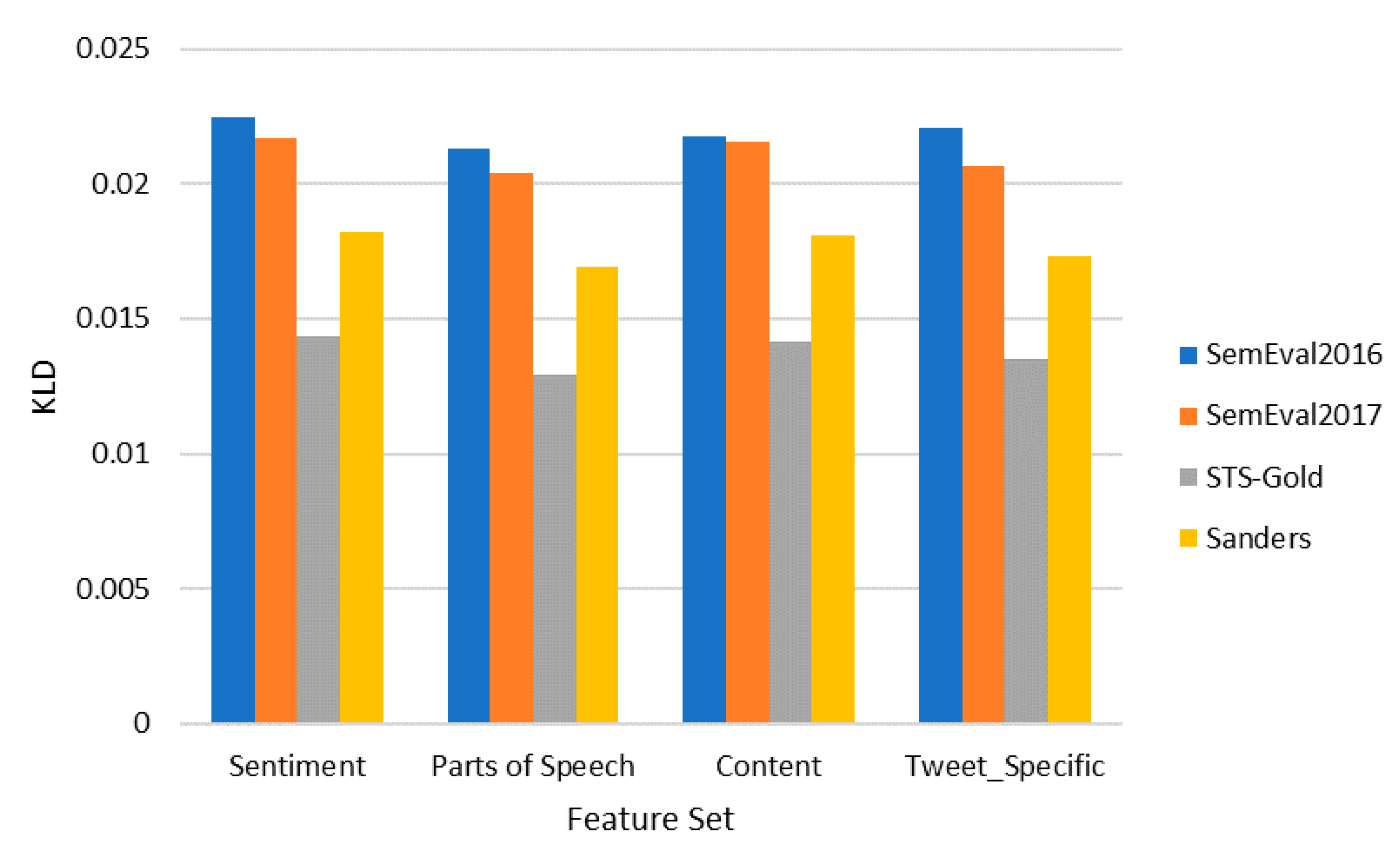
4.1. Single Feature Sets
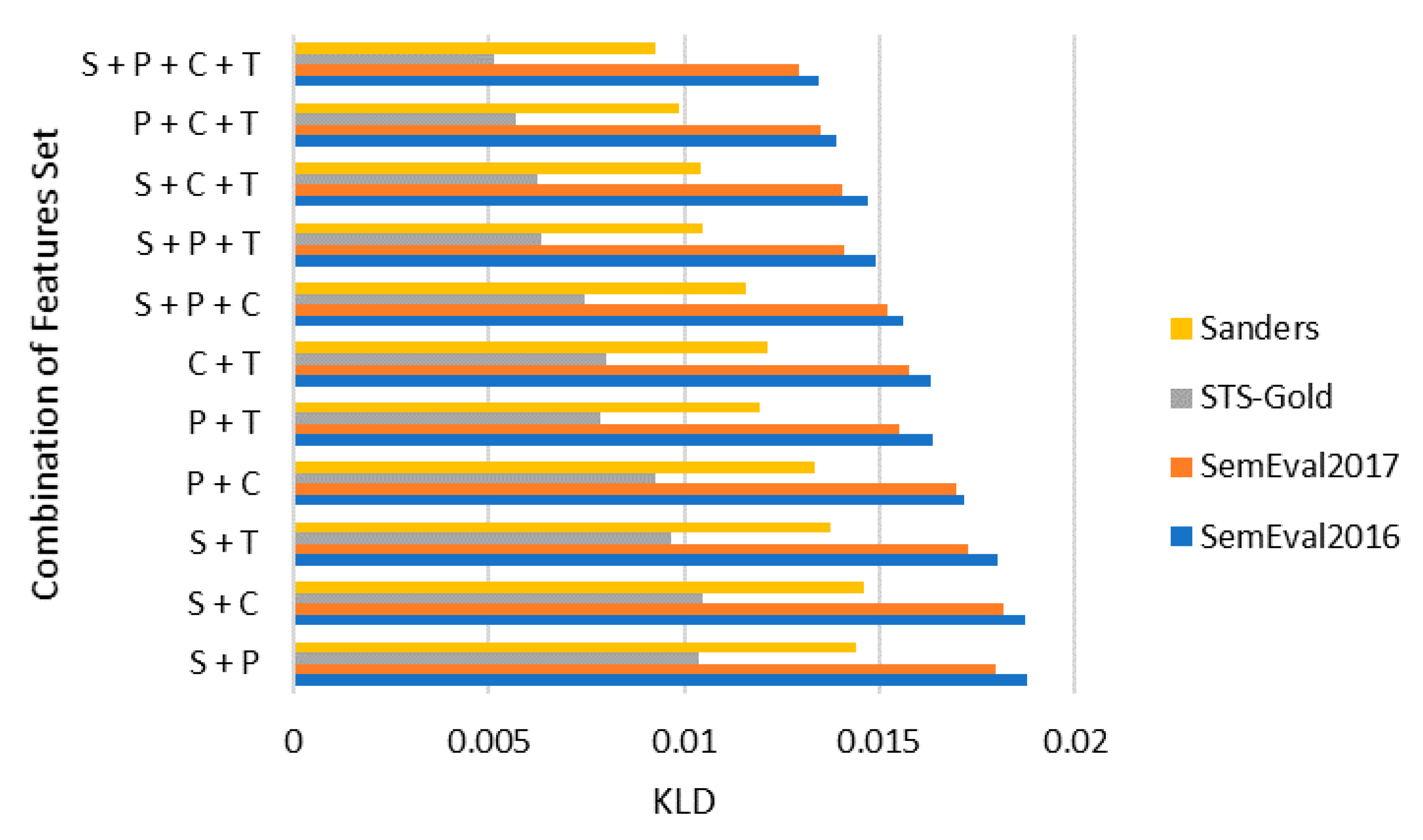
4.2. Combination of Feature Sets
4.3. Optimal Feature Sets
4.4. Results of Deep Features
4.5. Comparison of Proposed Technique with Existing Techniques
5. Conclusions
- As the social web channels provide a facility to add multilingual content, it raises diverse research issues for natural language processing and context understanding. In the case of multilingual content, especially where the diversity in different languages’ structure presents issues such as sentence structure, stemming, parsing, tagging, etc., more research is needed.
- Each language has its own syntax and vocabulary. Text-based features of each language provide different research challenges. Therefore, applying the proposed features and algorithms on languages such as Arabic, Persian, and Urdu will be an interesting research work, as these languages are written from right to left.
- The analysis and learning carried out using one language can be applied to another language using cross-lingual analysis. Thus, the cross-lingual sentiment quantification task can also be a potential research area, especially in languages that lack annotated datasets.
Author Contributions
Funding
Data Availability Statement
Conflicts of Interest
References
- Zamir, A.; Khan, H.U.; Mehmood, W.; Iqbal, T.; Akram, A.U. A feature-centric spam email detection model using diverse supervised machine learning algorithms. Electron. Libr. 2020, 38, 633–657. [Google Scholar] [CrossRef]
- Mahmood, A.; Khan, H.U.; Ramzan, M.J. On Modelling for Bias-Aware Sentiment Analysis and Its Impact in Twitter. J. Web Eng. 2020, 1–28, 21–28. [Google Scholar]
- Jabreel, M.; Moreno, A.J.A.S. A deep learning-based approach for multi-label emotion classification in tweets. Appl. Sci. 2019, 9, 1123. [Google Scholar] [CrossRef] [Green Version]
- Chen, C.Y.-H.; Hafner, C.M.J. Sentiment-induced bubbles in the cryptocurrency market. J. Risk Insur. 2019, 12, 53. [Google Scholar] [CrossRef] [Green Version]
- Jungherr, A.; Schoen, H.; Posegga, O.; Jürgens, P. Digital trace data in the study of public opinion: An indicator of attention toward politics rather than political support. Soc. Sci. Comput. Rev. 2017, 35, 336–356. [Google Scholar] [CrossRef] [Green Version]
- Rosenthal, S.; Farra, N.; Nakov, P. SemEval-2017 task 4: Sentiment analysis in Twitter. In Proceedings of the Proceedings of the 11th international workshop on semantic evaluation (SemEval-2017), Vancouver, BC, Canada, 4 August 2017; pp. 502–518. [Google Scholar]
- Gao, W.; Sebastiani, F. From classification to quantification in tweet sentiment analysis. Soc. Net. Anal. Min. 2016, 6, 1–22. [Google Scholar] [CrossRef]
- Moradi-Jamei, B.; Shakeri, H.; Poggi-Corradini, P.; Higgins, M.J. A new method for quantifying network cyclic structure to improve community detection. Physica A 2021, 561, 125116. [Google Scholar] [CrossRef]
- Esuli, A.; Moreo, A.; Sebastiani, F. Cross-lingual sentiment quantification. IEEE Intell. Syst. 2020, 35, 106–114. [Google Scholar] [CrossRef]
- Faryal, M.; Iqbal, M.; Tahreem, H. Mental health diseases analysis on Twitter using machine learning. IKSP J. Comput. Sci. Eng. 2021, 1, 16–25. [Google Scholar]
- Samuel, J.; Ali, G.; Rahman, M.; Esawi, E.; Samuel, Y. COVID-19 public sentiment insights and machine learning for tweets classification. Information 2020, 11, 314. [Google Scholar] [CrossRef]
- Hassan, W.; Maletzke, A.; Batista, G. Accurately quantifying a billion instances per second. In Proceedings of the 2020 IEEE 7th International Conference on Data Science and Advanced Analytics (DSAA), Sydney, Australia, 6 October 2020; pp. 1–10. [Google Scholar]
- Da San Martino, G.; Gao, W.; Sebastiani, F. Ordinal text quantification. In Proceedings of the 39th International ACM SIGIR conference on Research and Development in Information Retrieval, Pisa, Italy, 7 July 2016; pp. 937–940. [Google Scholar]
- Solyman, A.; Zhenyu, W.; Qian, T.; Elhag, A.A.M.; Rui, Z.; Mahmoud, Z. Automatic Arabic Grammatical Error Correction based on Expectation Maximization routing and target-bidirectional agreement. Know.-Based Syst. 2022, 241, 108180. [Google Scholar] [CrossRef]
- Alzanin, S.M.; Azmi, A.M. Rumor detection in Arabic tweets using semi-supervised and unsupervised expectation–maximization. Know.-Based Syst. 2019, 185, 104945. [Google Scholar] [CrossRef]
- Daughton, A.R.; Paul, M. A bootstrapping approach to social media quantification. Soc. Net. Anal. Min. 2021, 11, 1–14. [Google Scholar] [CrossRef]
- Esuli, A.; Moreo Fernández, A.; Sebastiani, F. A recurrent neural network for sentiment quantification. In Proceedings of the 27th ACM International Conference on Information and Knowledge Management, Torino, Italy, 17 October 2018; pp. 1775–1778. [Google Scholar]
- González-Castro, V.; Alaiz-Rodríguez, R.; Alegre, E. Class distribution estimation based on the Hellinger distance. Inf. Sci. 2013, 218, 146–164. [Google Scholar] [CrossRef]
- Hopkins, D.J.; King, G.J.A.J.o.P.S. A method of automated nonparametric content analysis for social science. Am. J. Political Sci. 2010, 54, 229–247. [Google Scholar] [CrossRef] [Green Version]
- Pérez-Gállego, P.; Castano, A.; Quevedo, J.R.; del Coz, J. Dynamic ensemble selection for quantification tasks. Inf. Fus. 2019, 45, 1–15. [Google Scholar] [CrossRef]
- Pérez-Gállego, P.; Quevedo, J.R.; del Coz, J. Using ensembles for problems with characterizable changes in data distribution: A case study on quantification. Inf. Fus. 2017, 34, 87–100. [Google Scholar] [CrossRef] [Green Version]
- Dias, F.F.; Ponti, M.A.; Minghim, R. A classification and quantification approach to generate features in soundscape ecology using neural networks. Neur. Comput. Appl. 2021, 34, 1–15. [Google Scholar] [CrossRef]
- Adarsh, R.; Patil, A.; Rayar, S.; Veena, K. Comparison of VADER and LSTM for sentiment analysis. Int. J. Recent Technol. Eng. 2019, 7, 540–543. [Google Scholar]
- Alabrah, A.; Alawadh, H.M.; Okon, O.D.; Meraj, T.; Rauf, H.T. Gulf Countries’ Citizens’ Acceptance of COVID-19 Vaccines—A Machine Learning Approach. Mathematics 2022, 10, 467. [Google Scholar] [CrossRef]
- Khan, H.U. Mixed-sentiment classification of web forum posts using lexical and non-lexical features. J. Web Eng. 2017, 16, 161–176. [Google Scholar]
- Khan, H.U.; Daud, A. Using Machine Learning Techniques for Subjectivity Analysis based on Lexical and Nonlexical Features. J. Web Eng. 2017, 14, 481–487. [Google Scholar]
- Almanaseer, W.; Alshraideh, M.; Alkadi, O. A deep belief network classification approach for automatic diacritization of arabic text. Appl. Sci. 2021, 11, 5228. [Google Scholar] [CrossRef]
- Elzayady, H.; Badran, K.M.; Salama, G.I. Arabic Opinion Mining Using Combined CNN-LSTM Models. Int. J. Intell. Syst. Appl. 2020, 12, 25–36. [Google Scholar] [CrossRef]
- Nemes, L.; Kiss, A.J. Social media sentiment analysis based on COVID-19. J. Inf. Syst. Telecommun. 2021, 5, 1–15. [Google Scholar] [CrossRef]
- Zeng, J.; Liu, T.; Jia, W.; Zhou, J. Relation construction for aspect-level sentiment classification. Inf. Sci. 2022, 586, 209–223. [Google Scholar] [CrossRef]
- Wu, C.; Xiong, Q.; Yi, H.; Yu, Y.; Zhu, Q.; Gao, M.; Chen, J. Multiple-element joint detection for Aspect-Based Sentiment Analysis. Knowl.-Based Syst. 2021, 223, 107073. [Google Scholar] [CrossRef]
- Pathak, A.R.; Pandey, M.; Rautaray, S. Topic-level sentiment analysis of social media data using deep learning. Appl. Soft Comput. 2021, 108, 107440. [Google Scholar] [CrossRef]
- Hamraoui, I.; Boubaker, A. Impact of Twitter sentiment on stock price returns. Soc. Net. Anal. Min. 2022, 12, 1–15. [Google Scholar] [CrossRef]
- Saif, H.; Fernandez, M.; He, Y.; Alani, H. Evaluation datasets for Twitter sentiment analysis: A survey and a new dataset, the STS-Gold. In Proceedings of the 1st Interantional Workshop on Emotion and Sentiment in Social and Expressive Media: Approaches and Perspectives from AI (ESSEM 2013), Turin, Italy, 3 December 2013. [Google Scholar]
- Wang, D.; Al-Rubaie, A.; Hirsch, B.; Pole, G.C. National happiness index monitoring using Twitter for bilanguages. Soc. Net. Anal. Min. 2021, 11, 1–18. [Google Scholar] [CrossRef]
- Deitrick, W.; Hu, W. Mutually enhancing community detection and sentiment analysis on twitter networks. J. Data Anal. Inf. Proc. 2013, 1, 19–29. [Google Scholar] [CrossRef] [Green Version]
- Nakov, P.; Ritter, A.; Rosenthal, S.; Sebastiani, F.; Stoyanov, V. SemEval-2016 task 4: Sentiment analysis in Twitter. arXiv 2019, arXiv:1912.00741. [Google Scholar]
- Ayyub, K.; Iqbal, S.; Munir, E.U.; Nisar, M.W.; Abbasi, M. Exploring diverse features for sentiment quantification using machine learning algorithms. IEEE Access 2020, 8, 142819–142831. [Google Scholar] [CrossRef]
- Labille, K.; Gauch, S. Optimizing Statistical Distance Measures in Multivariate SVM for Sentiment Quantification. In Proceedings of the the Thirteenth International Conference on Information, Process, and Knowledge Management, Nice, France, 18–22 July 2021; pp. 57–64. [Google Scholar]

| Method | Approach | Year | Feature(s) | Dataset |
|---|---|---|---|---|
| Aggregated | Expectation Minimization (EM) [15] | 2022 | User and content-based features. | Tweets |
| Expectation Minimization (EM) [14] | 2022 | Quantifying errors in text | QALB-2014, QALB-2015 | |
| Sample Means Matching (SMM) [12] | 2020 | Quantifying billions of data elements in seconds. | 25 benchmark datasets | |
| QuaNet [17] | 2018 | Quantification of data. | Kindle, IMDb, HP (Harry Potter) | |
| OQT [13] | 2016 | Quantifying Tweets | SemEval2016 | |
| Non-Aggregated | Automated Nonparametric Content Analysis [18] | 2010 | Quantification of data. | Blogs |
| HDy and HDx [18] | 2013 | Quantification of data. | UCI datasets | |
| Ensemble-based | Ensembles for Quantification [21] | 2017 | Data distribution and quantification. | UCI datasets, Sentiment140 |
| Dynamic Ensembles [20] | 2019 | Quantification of data. Applied techniques based on ensemble learners. | UCI datasets |
| Sr# | Categories | Description | Symbol |
|---|---|---|---|
| 1 | Sentiment | Sentiment score of the tweet | |
| 2 | Sentiment—Number of positive words | ||
| 3 | Sentiment—Number of negative words | ||
| 4 | Count of positive emoticons | ||
| 5 | Count of negative emoticons | ||
| 6 | POS | Number of nouns in a tweet | |
| 7 | Number of pronouns in a tweet | ||
| 8 | Verbs frequency in a tweet | ||
| 9 | Adjectives frequency in a tweet | ||
| 10 | Content | Number of special symbols | |
| 11 | Number of WH words in a tweet | ||
| 12 | Number of question marks in a tweet | ||
| 13 | Number of exclamation marks | ||
| 14 | Number of capitalized words | ||
| 15 | Number of quoted words | ||
| 16 | Tweet Specific | Number of retweets | |
| 17 | Number of mentions | ||
| 18 | Number of URLs | ||
| 19 | Hashtag length | ||
| 20 | Is it a tweet or retweet? | ||
| 21 | Number of hashtags | ||
| 22 | Number of capitalized hashtags |
| Sentiment | Parts of Speech | Content | Tweet Specific | Baseline | Deep |
|---|---|---|---|---|---|
| Sentiment score of the tweet | Verbs frequency in a tweet | Number of WH words in a tweet | Number of mentions | TF-IDF | GloVe |
| Sentiment—Number of negative words | Adjectives frequency in a tweet | Number of question marks in a tweet | Number of retweets | n-gram | Word2vec |
| Sentiment—Number of positive words | Number of nouns in a tweet | Number of quoted words | Number of URLs | BoW | |
| Count of negative emoticons | Number of pronouns in a tweet | Number of repetitive words | Number of hashtags | ||
| Count of positive emoticons | Number of special symbols | Number of capitalized hashtags | |||
| Number of exclamation marks | Hashtag length | ||||
| Is it a tweet or retweet? |
| Dataset | Total Tweets | Testing Tweets | Training Tweets |
|---|---|---|---|
| SemEval2016 | 68,197 | 51,851 | 16,346 |
| SemEval2017 | 62,617 | 12,284 | 50,333 |
| STS-Gold | 1,600,000 | 320,000 | 1,280,000 |
| Sanders | 5512 | 1102 | 4410 |
| Dataset | Features | NB | DT | SVM | AdaBoost | RF | ||||||||||
|---|---|---|---|---|---|---|---|---|---|---|---|---|---|---|---|---|
| AE | RAE | KLD | AE | RAE | KLD | AE | RAE | KLD | AE | RAE | KLD | AE | RAE | KLD | ||
| SemEval2016 | S | 0.033 | 0.691 | 0.025 | 0.040 | 0.798 | 0.030 | 0.030 | 0.599 | 0.023 | 0.029 | 0.595 | 0.022 | 0.030 | 0.634 | 0.023 |
| P | 0.044 | 0.898 | 0.034 | 0.037 | 0.750 | 0.028 | 0.028 | 0.575 | 0.022 | 0.028 | 0.571 | 0.021 | 0.042 | 0.853 | 0.032 | |
| C | 0.039 | 0.802 | 0.030 | 0.035 | 0.708 | 0.026 | 0.029 | 0.579 | 0.022 | 0.036 | 0.715 | 0.027 | 0.037 | 0.750 | 0.028 | |
| T | 0.055 | 1.097 | 0.042 | 0.029 | 0.603 | 0.022 | 0.029 | 0.596 | 0.022 | 0.029 | 0.592 | 0.022 | 0.053 | 1.056 | 0.040 | |
| SemEval2017 | S | 0.030 | 0.618 | 0.022 | 0.041 | 0.823 | 0.031 | 0.029 | 0.577 | 0.022 | 0.028 | 0.576 | 0.022 | 0.035 | 0.732 | 0.026 |
| P | 0.049 | 0.986 | 0.037 | 0.035 | 0.710 | 0.027 | 0.028 | 0.572 | 0.021 | 0.027 | 0.547 | 0.020 | 0.030 | 0.607 | 0.023 | |
| C | 0.043 | 0.873 | 0.032 | 0.032 | 0.657 | 0.025 | 0.028 | 0.574 | 0.022 | 0.033 | 0.671 | 0.026 | 0.032 | 0.657 | 0.024 | |
| T | 0.072 | 1.453 | 0.056 | 0.027 | 0.565 | 0.021 | 0.028 | 0.575 | 0.022 | 0.028 | 0.572 | 0.021 | 0.029 | 0.579 | 0.022 | |
| STS-Gold | S | 0.021 | 0.434 | 0.016 | 0.033 | 0.661 | 0.025 | 0.019 | 0.378 | 0.014 | 0.019 | 0.378 | 0.014 | 0.027 | 0.566 | 0.020 |
| P | 0.042 | 0.851 | 0.032 | 0.026 | 0.532 | 0.020 | 0.018 | 0.375 | 0.014 | 0.017 | 0.347 | 0.013 | 0.020 | 0.413 | 0.016 | |
| C | 0.035 | 0.723 | 0.027 | 0.023 | 0.472 | 0.018 | 0.019 | 0.376 | 0.014 | 0.024 | 0.485 | 0.019 | 0.023 | 0.473 | 0.018 | |
| T | 0.069 | 1.385 | 0.053 | 0.018 | 0.370 | 0.014 | 0.019 | 0.377 | 0.014 | 0.018 | 0.374 | 0.014 | 0.019 | 0.380 | 0.015 | |
| Sanders | S | 0.025 | 0.532 | 0.019 | 0.037 | 0.748 | 0.028 | 0.024 | 0.484 | 0.018 | 0.024 | 0.483 | 0.018 | 0.031 | 0.655 | 0.023 |
| P | 0.045 | 0.923 | 0.035 | 0.031 | 0.627 | 0.024 | 0.024 | 0.480 | 0.018 | 0.022 | 0.454 | 0.017 | 0.026 | 0.517 | 0.020 | |
| C | 0.039 | 0.803 | 0.030 | 0.028 | 0.571 | 0.021 | 0.024 | 0.482 | 0.018 | 0.029 | 0.584 | 0.022 | 0.028 | 0.571 | 0.021 | |
| T | 0.071 | 1.421 | 0.054 | 0.023 | 0.474 | 0.017 | 0.024 | 0.482 | 0.018 | 0.024 | 0.479 | 0.018 | 0.024 | 0.486 | 0.019 | |
| Features | NB | DT | SVM | AdaBoost | RF | ||||||||||
|---|---|---|---|---|---|---|---|---|---|---|---|---|---|---|---|
| AE | RAE | KLD | AE | RAE | KLD | AE | RAE | KLD | AE | RAE | KLD | AE | RAE | KLD | |
| SP | 0.036 | 0.736 | 0.027 | 0.035 | 0.713 | 0.027 | 0.025 | 0.519 | 0.019 | 0.025 | 0.512 | 0.019 | 0.033 | 0.680 | 0.025 |
| SC | 0.032 | 0.671 | 0.024 | 0.033 | 0.679 | 0.025 | 0.025 | 0.506 | 0.019 | 0.028 | 0.575 | 0.022 | 0.029 | 0.613 | 0.022 |
| ST | 0.040 | 0.824 | 0.031 | 0.030 | 0.611 | 0.022 | 0.024 | 0.499 | 0.018 | 0.024 | 0.494 | 0.018 | 0.038 | 0.773 | 0.029 |
| PC | 0.037 | 0.758 | 0.028 | 0.031 | 0.630 | 0.023 | 0.023 | 0.467 | 0.017 | 0.026 | 0.537 | 0.020 | 0.034 | 0.705 | 0.026 |
| PT | 0.045 | 0.916 | 0.035 | 0.027 | 0.558 | 0.020 | 0.022 | 0.461 | 0.017 | 0.022 | 0.454 | 0.016 | 0.043 | 0.869 | 0.033 |
| CT | 0.042 | 0.850 | 0.032 | 0.025 | 0.523 | 0.019 | 0.022 | 0.448 | 0.016 | 0.025 | 0.520 | 0.019 | 0.039 | 0.801 | 0.030 |
| SPC | 0.032 | 0.664 | 0.024 | 0.030 | 0.617 | 0.023 | 0.021 | 0.431 | 0.016 | 0.023 | 0.477 | 0.017 | 0.029 | 0.606 | 0.022 |
| SPT | 0.037 | 0.769 | 0.028 | 0.027 | 0.565 | 0.021 | 0.020 | 0.423 | 0.015 | 0.020 | 0.418 | 0.015 | 0.035 | 0.716 | 0.026 |
| SCT | 0.035 | 0.719 | 0.026 | 0.026 | 0.538 | 0.019 | 0.020 | 0.410 | 0.015 | 0.022 | 0.457 | 0.017 | 0.032 | 0.663 | 0.024 |
| PCT | 0.038 | 0.788 | 0.029 | 0.024 | 0.505 | 0.018 | 0.019 | 0.389 | 0.014 | 0.021 | 0.436 | 0.016 | 0.036 | 0.736 | 0.027 |
| SPCT | 0.034 | 0.706 | 0.025 | 0.025 | 0.524 | 0.019 | 0.018 | 0.379 | 0.014 | 0.020 | 0.412 | 0.015 | 0.031 | 0.649 | 0.023 |
| Features | NB | DT | SVM | AdaBoost | RF | ||||||||||
|---|---|---|---|---|---|---|---|---|---|---|---|---|---|---|---|
| AE | RAE | KLD | AE | RAE | KLD | AE | RAE | KLD | AE | RAE | KLD | AE | RAE | KLD | |
| SP | 0.036 | 0.742 | 0.027 | 0.035 | 0.705 | 0.027 | 0.025 | 0.505 | 0.019 | 0.024 | 0.489 | 0.018 | 0.029 | 0.606 | 0.022 |
| SC | 0.032 | 0.669 | 0.024 | 0.033 | 0.665 | 0.025 | 0.024 | 0.491 | 0.018 | 0.027 | 0.542 | 0.020 | 0.029 | 0.617 | 0.022 |
| ST | 0.048 | 0.971 | 0.036 | 0.029 | 0.604 | 0.022 | 0.023 | 0.476 | 0.018 | 0.023 | 0.473 | 0.017 | 0.028 | 0.575 | 0.022 |
| PC | 0.041 | 0.843 | 0.031 | 0.028 | 0.581 | 0.022 | 0.022 | 0.462 | 0.017 | 0.024 | 0.501 | 0.019 | 0.026 | 0.525 | 0.019 |
| PT | 0.057 | 1.157 | 0.044 | 0.025 | 0.517 | 0.019 | 0.022 | 0.448 | 0.016 | 0.021 | 0.431 | 0.016 | 0.024 | 0.475 | 0.018 |
| CT | 0.053 | 1.083 | 0.041 | 0.023 | 0.474 | 0.017 | 0.021 | 0.434 | 0.016 | 0.024 | 0.486 | 0.018 | 0.024 | 0.489 | 0.018 |
| SPC | 0.033 | 0.695 | 0.025 | 0.029 | 0.593 | 0.022 | 0.020 | 0.420 | 0.015 | 0.022 | 0.445 | 0.016 | 0.025 | 0.521 | 0.019 |
| SPT | 0.044 | 0.903 | 0.033 | 0.026 | 0.546 | 0.020 | 0.020 | 0.406 | 0.015 | 0.019 | 0.395 | 0.014 | 0.024 | 0.488 | 0.018 |
| SCT | 0.041 | 0.848 | 0.031 | 0.025 | 0.514 | 0.019 | 0.019 | 0.392 | 0.014 | 0.021 | 0.427 | 0.016 | 0.024 | 0.492 | 0.018 |
| PCT | 0.048 | 0.981 | 0.036 | 0.022 | 0.457 | 0.016 | 0.018 | 0.378 | 0.014 | 0.019 | 0.403 | 0.015 | 0.021 | 0.430 | 0.016 |
| SPCT | 0.040 | 0.829 | 0.030 | 0.024 | 0.495 | 0.018 | 0.017 | 0.364 | 0.013 | 0.018 | 0.383 | 0.014 | 0.022 | 0.450 | 0.016 |
| Features | NB | DT | SVM | AdaBoost | RF | ||||||||||
|---|---|---|---|---|---|---|---|---|---|---|---|---|---|---|---|
| AE | RAE | KLD | AE | RAE | KLD | AE | RAE | KLD | AE | RAE | KLD | AE | RAE | KLD | |
| SP | 0.028 | 0.575 | 0.021 | 0.026 | 0.528 | 0.020 | 0.015 | 0.299 | 0.011 | 0.014 | 0.283 | 0.010 | 0.020 | 0.419 | 0.015 |
| SC | 0.024 | 0.494 | 0.018 | 0.024 | 0.483 | 0.018 | 0.014 | 0.283 | 0.010 | 0.017 | 0.340 | 0.013 | 0.021 | 0.434 | 0.015 |
| ST | 0.041 | 0.835 | 0.031 | 0.020 | 0.414 | 0.015 | 0.013 | 0.267 | 0.010 | 0.013 | 0.265 | 0.010 | 0.019 | 0.379 | 0.014 |
| PC | 0.033 | 0.691 | 0.025 | 0.019 | 0.387 | 0.014 | 0.012 | 0.252 | 0.009 | 0.014 | 0.294 | 0.011 | 0.016 | 0.323 | 0.012 |
| PT | 0.052 | 1.046 | 0.040 | 0.015 | 0.316 | 0.011 | 0.011 | 0.236 | 0.009 | 0.010 | 0.219 | 0.008 | 0.013 | 0.261 | 0.010 |
| CT | 0.047 | 0.963 | 0.036 | 0.013 | 0.270 | 0.010 | 0.011 | 0.220 | 0.008 | 0.014 | 0.278 | 0.010 | 0.014 | 0.279 | 0.010 |
| SPC | 0.025 | 0.524 | 0.019 | 0.020 | 0.402 | 0.015 | 0.010 | 0.205 | 0.007 | 0.011 | 0.234 | 0.009 | 0.015 | 0.325 | 0.012 |
| SPT | 0.037 | 0.759 | 0.028 | 0.017 | 0.349 | 0.013 | 0.009 | 0.190 | 0.007 | 0.009 | 0.178 | 0.006 | 0.014 | 0.281 | 0.010 |
| SCT | 0.034 | 0.698 | 0.025 | 0.015 | 0.314 | 0.011 | 0.008 | 0.174 | 0.006 | 0.010 | 0.213 | 0.008 | 0.014 | 0.288 | 0.010 |
| PCT | 0.041 | 0.847 | 0.031 | 0.012 | 0.251 | 0.009 | 0.008 | 0.159 | 0.006 | 0.009 | 0.188 | 0.007 | 0.010 | 0.214 | 0.008 |
| SPCT | 0.032 | 0.676 | 0.024 | 0.014 | 0.294 | 0.011 | 0.007 | 0.144 | 0.005 | 0.008 | 0.165 | 0.006 | 0.012 | 0.241 | 0.009 |
| Features | NB | DT | SVM | AdaBoost | RF | ||||||||||
|---|---|---|---|---|---|---|---|---|---|---|---|---|---|---|---|
| AE | RAE | KLD | AE | RAE | KLD | AE | RAE | KLD | AE | RAE | KLD | AE | RAE | KLD | |
| SP | 0.032 | 0.665 | 0.024 | 0.031 | 0.622 | 0.023 | 0.020 | 0.409 | 0.015 | 0.019 | 0.393 | 0.014 | 0.025 | 0.519 | 0.019 |
| SC | 0.028 | 0.588 | 0.021 | 0.028 | 0.580 | 0.022 | 0.019 | 0.394 | 0.015 | 0.022 | 0.447 | 0.017 | 0.025 | 0.532 | 0.019 |
| ST | 0.044 | 0.908 | 0.034 | 0.025 | 0.515 | 0.019 | 0.018 | 0.379 | 0.014 | 0.018 | 0.376 | 0.014 | 0.024 | 0.484 | 0.018 |
| PC | 0.037 | 0.772 | 0.028 | 0.024 | 0.491 | 0.018 | 0.018 | 0.364 | 0.013 | 0.020 | 0.404 | 0.015 | 0.021 | 0.431 | 0.016 |
| PT | 0.055 | 1.105 | 0.042 | 0.020 | 0.423 | 0.015 | 0.017 | 0.349 | 0.013 | 0.016 | 0.332 | 0.012 | 0.019 | 0.375 | 0.014 |
| CT | 0.050 | 1.027 | 0.038 | 0.018 | 0.379 | 0.014 | 0.016 | 0.334 | 0.012 | 0.019 | 0.389 | 0.014 | 0.019 | 0.391 | 0.015 |
| SPC | 0.029 | 0.615 | 0.022 | 0.025 | 0.504 | 0.019 | 0.015 | 0.320 | 0.012 | 0.017 | 0.347 | 0.013 | 0.020 | 0.430 | 0.015 |
| SPT | 0.041 | 0.836 | 0.031 | 0.022 | 0.454 | 0.017 | 0.015 | 0.305 | 0.011 | 0.014 | 0.294 | 0.010 | 0.019 | 0.392 | 0.014 |
| SCT | 0.037 | 0.778 | 0.028 | 0.020 | 0.420 | 0.015 | 0.014 | 0.290 | 0.010 | 0.016 | 0.327 | 0.012 | 0.019 | 0.397 | 0.014 |
| PCT | 0.045 | 0.918 | 0.034 | 0.017 | 0.361 | 0.013 | 0.013 | 0.276 | 0.010 | 0.014 | 0.303 | 0.011 | 0.016 | 0.329 | 0.012 |
| SPCT | 0.036 | 0.758 | 0.027 | 0.019 | 0.401 | 0.014 | 0.012 | 0.262 | 0.009 | 0.013 | 0.281 | 0.010 | 0.017 | 0.352 | 0.013 |
| Algorithm | Features | SemEval2016 | SemEval2017 | STS-Gold | Sanders | ||||||||
|---|---|---|---|---|---|---|---|---|---|---|---|---|---|
| AE | RAE | KLD | AE | RAE | KLD | AE | RAE | KLD | AE | RAE | KLD | ||
| DBN | GloVe | 0.019 | 0.394 | 0.014 | 0.021 | 0.431 | 0.015 | 0.011 | 0.222 | 0.008 | 0.016 | 0.334 | 0.012 |
| Word2vec | 0.020 | 0.423 | 0.015 | 0.024 | 0.496 | 0.018 | 0.014 | 0.296 | 0.011 | 0.019 | 0.403 | 0.014 | |
| n-Gram | 0.033 | 0.676 | 0.025 | 0.034 | 0.695 | 0.026 | 0.025 | 0.516 | 0.019 | 0.030 | 0.612 | 0.023 | |
| BoW | 0.036 | 0.717 | 0.027 | 0.034 | 0.686 | 0.026 | 0.025 | 0.503 | 0.019 | 0.030 | 0.601 | 0.023 | |
| CNN-LSTM | GloVe | 0.014 | 0.298 | 0.011 | 0.016 | 0.345 | 0.012 | 0.006 | 0.122 | 0.004 | 0.011 | 0.241 | 0.009 |
| Word2vec | 0.016 | 0.329 | 0.012 | 0.019 | 0.393 | 0.014 | 0.037 | 0.772 | 0.027 | 0.037 | 0.772 | 0.027 | |
| n-Gram | 0.030 | 0.602 | 0.023 | 0.031 | 0.624 | 0.023 | 0.021 | 0.435 | 0.016 | 0.026 | 0.536 | 0.020 | |
| BoW | 0.030 | 0.606 | 0.023 | 0.030 | 0.602 | 0.023 | 0.020 | 0.409 | 0.015 | 0.025 | 0.512 | 0.019 | |
| RNN | GloVe | 0.012 | 0.256 | 0.009 | 0.015 | 0.308 | 0.011 | 0.037 | 0.772 | 0.027 | 0.037 | 0.772 | 0.027 |
| Word2vec | 0.015 | 0.306 | 0.011 | 0.016 | 0.338 | 0.012 | 0.005 | 0.114 | 0.004 | 0.011 | 0.234 | 0.008 | |
| n-Gram | 0.029 | 0.587 | 0.022 | 0.029 | 0.599 | 0.022 | 0.046 | 0.935 | 0.035 | 0.046 | 0.935 | 0.035 | |
| BoW | 0.027 | 0.565 | 0.021 | 0.028 | 0.568 | 0.021 | 0.045 | 0.928 | 0.034 | 0.045 | 0.928 | 0.034 | |
| Sr. No | Dataset | Proposed Method | Baseline | Reference |
|---|---|---|---|---|
| 1 | SemEval2016 | KLD = 0.013 | KLD = 0.034 | [37] |
| 2 | SemEval2017 | KLD = 0.012 | KLD = 0.036 | [6] |
| 3 | STS-Gold | AE = 0.007 | AE = 0.008 | [38] |
| 4 | Sanders | KLD = 0.010 | KLD = 0.009 | [39] |
| Algorithms | Values |
|---|---|
| NB | priors = None, var_smoothing = 1e-09 |
| Decision Tree | (loss = “deviance”, learning_rate = 0.01, n_estimators = 100, subsample = 1.0, criterion = “friedman_mse”, min_samples_split = 2, min_samples_leaf = 1, min_weight_fraction_leaf = 0.0, max_depth = 3, min_impurity_decrease = 0.0, min_impurity_split = None, init = None, random_state = None, max_features = None, verbose = 0, max_leaf_nodes = None, warm_start = False, presort = “auto”, validation_fraction = 0.1, n_iter_no_change = None, tol = 0.0001) |
| SVM | C = 1.0, kernel = “rbf”, degree = 3, gamma = “auto_deprecated”, coef0 = 0.0, shrinking = True, probability = False, tol = 0.001, cache_size = 200, class_weight = None, verbose = False, max_iter = 1, decision_function_shape = “ovr”, random_state = None |
| AdaBoost | (base_estimator = None, n_estimators = 10, max_samples = 1.0, max_features = 1.0, bootstrap = True, bootstrap_features = False, oob_score = False, warm_start = False, n_jobs = None, random_state = None, |
| RF | (n_estimators = 10, criterion = “gini”, max_depth = None, min_samples_split = 2, min_samples_leaf = 1, min_weight_fraction_leaf = 0.0, max_features = “auto”, max_leaf_nodes = None, min_impurity_decrease = 0.0, min_impurity_split = None, bootstrap = True, oob_score = False, n_jobs = None, random_state = None, verbose = 0, warm_start = False, class_weight = None) |
Publisher’s Note: MDPI stays neutral with regard to jurisdictional claims in published maps and institutional affiliations. |
© 2022 by the authors. Licensee MDPI, Basel, Switzerland. This article is an open access article distributed under the terms and conditions of the Creative Commons Attribution (CC BY) license (https://creativecommons.org/licenses/by/4.0/).
Share and Cite
Ayyub, K.; Iqbal, S.; Wasif Nisar, M.; Munir, E.U.; Alarfaj, F.K.; Almusallam, N. A Feature-Based Approach for Sentiment Quantification Using Machine Learning. Electronics 2022, 11, 846. https://doi.org/10.3390/electronics11060846
Ayyub K, Iqbal S, Wasif Nisar M, Munir EU, Alarfaj FK, Almusallam N. A Feature-Based Approach for Sentiment Quantification Using Machine Learning. Electronics. 2022; 11(6):846. https://doi.org/10.3390/electronics11060846
Chicago/Turabian StyleAyyub, Kashif, Saqib Iqbal, Muhammad Wasif Nisar, Ehsan Ullah Munir, Fawaz Khaled Alarfaj, and Naif Almusallam. 2022. "A Feature-Based Approach for Sentiment Quantification Using Machine Learning" Electronics 11, no. 6: 846. https://doi.org/10.3390/electronics11060846
APA StyleAyyub, K., Iqbal, S., Wasif Nisar, M., Munir, E. U., Alarfaj, F. K., & Almusallam, N. (2022). A Feature-Based Approach for Sentiment Quantification Using Machine Learning. Electronics, 11(6), 846. https://doi.org/10.3390/electronics11060846