Article

Hybrid Differential Evolution-Based Regression Tree Model for Predicting Downstream Dam Hazard Potential

by
Eslam Mohammed Abdelkader
1,
Abobakr Al-Sakkaf
2,3,*,
Ghasan Alfalah
4 and
Nehal Elshaboury
5
1
Structural Engineering Department, Faculty of Engineering, Cairo University, Giza 12613, Egypt
2
Department of Buildings, Civil and Environmental Engineering, Concordia University, Montreal, QC H3G 1M8, Canada
3
Department of Architecture & Environmental Planning, College of Engineering & Petroleum, Hadhramout University, Mukalla 50512, Yemen
4
Department of Architecture and Building Science, College of Architecture and Planning, King Saud University, Riyadh 11421, Saudi Arabia
5
Housing and Building National Research Centre, Construction and Project Management Research Institute, Giza 12311, Egypt
*
Author to whom correspondence should be addressed.
Sustainability 2022, 14(5), 3013; https://doi.org/10.3390/su14053013
Submission received: 9 February 2022 / Revised: 26 February 2022 / Accepted: 2 March 2022 / Published: 4 March 2022

Abstract

:
There are a large number of dams throughout the United States, and a considerable portion of them are categorized as having high hazard potential. This state of affairs constitutes a challenge, especially when coupled with their rapid deterioration. As such, this research paper proposes an optimized data-driven model for the fast and efficient prediction of dam hazard potential. The proposed model is envisioned on two main components, namely model development and model assessment. In the first component, a hybridization of the differential evolution algorithm and regression tree to forecast downstream dam hazard potential is proposed. In this context, the differential evolution (DE) algorithm is deployed to: (1) automatically retrieve the optimal set of input features affecting dam hazard potential; and (2) amplify the search mechanism of regression tree (REGT) through optimizing its hyper parameters. As for the second component, the developed DE-REGT model is validated using four folds of comparative assessments to evaluate its prediction capabilities. In the first fold, the developed DE-REGT model is trialed against nine highly regarded machine learning and deep learning models. The second fold is designated to structure, an integrative ranking of the investigated data-driven models, counting on their scores in the performance evaluation metrics. The third fold is used to study the effectiveness of using differential evolution for the hyper parameter optimization of regression tree. The fourth fold aims at testing the usefulness of using differential evolution as a feature extractor algorithm. Performance comparative analysis demonstrated that the developed DE-REGT model outperformed the remainder of the data-driven models. It accomplished mean absolute percentage error, relative absolute error, mean absolute error, root squared error, root mean squared error and a Nash–Sutcliffe efficiency of 9.62%, 0.27, 0.17, 0.31, 0.41 and 0.74, respectively. Results also revealed that the developed model managed to perform better than other meta-heuristic-based regression tree models and classical feature extraction algorithms, exemplifying the appropriateness of using differential evolution for hyper parameter optimization and feature extraction. It can be argued that the developed model could assist policy makers in the prioritization of their maintenance management plans and reduce impairments caused by the failure or misoperation of dams.

1. Introduction

Dams play an integral role in the sustainment and economic development of countries [1]. It is reported that there are more than 91,000 dams in the United States that are registered in the National Inventory of Dams (NID). Their average age is 61 years, and 75% of them are identified as high hazard potential dams with emergency action plans [2]. Dams in the United States are suspectable to higher deterioration rates, their overall condition is “D”, and it is expected that seven out of ten bridges will exhibit an average age over 50 years old by 2030 [3]. In order to maintain the performance condition of dams and prevent them from further deterioration, $20 billion is needed to rehabilitate high hazard potential dams, and a cost estimate of nearly $66 billion is required to rehabilitate non-federal dams.
Dam failure could cause catastrophic damages to the economy, the environment, properties, and instigate the loss of human life [4,5,6]. The failure rate of dams surpassed 25 failures per year after 2010, and more than 72% of the failures took place for dams that were less than 70 years old. In addition, it was found that 4% of dam failures between 1850 and 2017 were linked with casualties, causing 3495 fatalities in total [7]. In this context, the hazard classification of dams is established based on the potential downstream consequences to property, business, life, and the environment [8,9]. As such, dam hazard classification was introduced to serve as a preliminary mechanism to plan maintenance and rehabilitation needs for existing dams through estimating the magnitude of dam failures. High hazard potential dams can be given the highest priority to be repaired [10,11,12]. Data-driven intelligent models have emerged in the last decade as a powerful growing mechanism that can improve asset management practices through boosting the asset’s performance condition and resilience and extending its service life. The reported data-driven models were implemented to a wide range of municipal infrastructure systems including water networks [13], sewer networks [14], roads [15], bridges [16] and highway tunnels [17]. In light of the foregoing, the main objectives of the present research study lie in the following:
  • To devise a hybrid differential evolution-based regression tree model for predicting the hazard potential of dams;
  • To validate the developed dam hazard potential prediction model against a set of widely acknowledged machine learning and deep learning models using performance evaluation comparisons.

2. Literature Review

In the last decades, some research studies have been carried out to analyze the hazard potential analysis of dams. Some models exploited the use of multi-criteria decision-making algorithms for assessing hazards and risks pertinent to dams. Xue et al. [18] proposed an integrated model for the rapid risk assessment of barrier dams, whereas two indicators of stability index and impact index were introduced to study the stability of barrier dams and the degree of significance after dam break. Fuzzy analytical hierarchy process was exploited to evaluate barrier dam stability and break influence. The stability index was measured according to dam height, storage capacity, and material composition of the dam body, while the impact index considered dam breakage degree, risk population, and potential economic loss. Daud et al. [19] explored the risk factors of dam failure using the analytical hierarchy process. In their hierarchy, the main criteria encompassed structural, human, and natural factors, whereas few sub-criteria were included under the main criteria. Structural criteria involved crack, settlement, erosion, seepage, etc. The human criteria incorporated vandalism, bombs, negligence, etc. The natural criteria contained landslide, flood from high precipitation, flood from dam failure, and earthquakes. It was found that seepage was the most influential contributor to dam failure, followed by operational mismanagement and then floods from high precipitation.
Guetz et al. [20] prioritized dams suitable for removal based on multi-criteria decision analysis. In this context, six categories were selected for dam removal prioritization which were: social, safety, connectivity, habitat, flow magnitude, and watershed alteration. Multi-attribute utility theory (MAUT) was implemented as a decision support system to identify and rank dams for removal. Celik and Gul [21] introduced a multi-criteria decision-making model for hazard assessment and control in dam construction. They targeted a set of risks such as unplanned fire or explosion, a selection of inadequate employees, the collision of vehicles, the overturning of vehicles and mobile plants, etc. In this regard, best worst method (BWM) is used to find the weights of risk parameters. In addition, interval type 2 fuzzy set is coupled with the measurement of alternatives and ranking according to compromise solution (MACROS) to set the relevant risks and hazards. It was observed that the most critical hazards in dam construction projects originate from driving vehicles and mobile plants.
He et al. [22] proposed an integrated fuzzy model to assess the social and environmental impacts of dam breaks. Their evaluation model considered a set of factors such as height of dam, water environment, soil environment, cultural heritage, level of city, vegetation damage, etc. Variable fuzzy sets were used to deal with uncertainties linked with the evaluation of dam breaks, and the analytical hierarchy process was used to derive the relative importance weights of the social and environmental aspects. It is illustrated that the accuracies of the developed evaluation model were improved through applying a synthetic membership degree. Ribas et al. [23] introduced a fuzzy-based model to assess the failure modes of the hydroelectric earth dam. Failure mode and effect analysis were merged to study the mechanisms that can cause potential damages to the dams. Fuzzy approximate reasoning was used to address the inherent accuracies associated with subjective estimates. A risk criticality index was created through merging the probabilities of occurrences and severities of failure modes.
Other studies opted to simulate the seismic risk scenarios of dams. Lu et al. [24] proposed a residual displacement-based seismic damage classification model for gravity dams. A linear mapping function was created between the residual displacement and peak ground acceleration based on the concrete damaged plasticity model under various earthquake waves. The considered loads in their damage classification model encompassed weight of dam body, uplift pressure, dynamic water pressure, upstream hydrostatic pressure, and seismic load. It was highlighted that displacement is an appropriate performance parameter for monitoring the safety behavior of dams. Li et al. [25] presented an improved model for the seismic risk analysis of gravity dams. In their model, the screening of intensity measures was merged with a surrogate artificial neural network to generate non-parametric fragility curves. Analytical results demonstrated that the simulated non-parametric fragility curves succeeded in simulating uncertainties of ground motions and providing a more accurate seismic risk analysis. Irinyemi et al. [26] conducted seismic hazard analysis for large dams based on the peak ground acceleration. In this regard, seismicity and geological features were used to appraise the seismic activity rate. In their seismic hazard analysis, seismic sources that yielded significant ground shaking were considered. The summation of capacity risk factor, height risk factor and age-rating risk factor were utilized to quantify the overall dam structure influence. Results of the study demonstrated that peak ground acceleration ranged from 0.31 to 0.52, with one large dam at high risk that needed to be inspected and monitored for seismic safety.
A third branch of studies dealt with monitoring the condition behavior of surface cracks in dams through digital imaging and deep learning algorithms. De Mello et al. [27] created a model for the inspection of concrete cracks in dams using a deep convolutional neural network. A faster region convolutional neural network and a single-shot multibox detector were used to identify nonconformities during the dam inspection process. Inception Resnet v2 was determined to be the premise of the developed object detection architecture, and the single-shot multibox detector was selected to be a feedforward convolutional network. The developed detection system was able to produce overall accuracy and an F1 score of 88.9%. Feng et al. [28] introduced an autonomous model for pixel-level crack detection on dam surfaces. The images were first collected using unmanned aerial vehicles, and then an improved SegNet architecture was utilized to identify the cracks. The encoding part of the improved SegNet architecture included fifteen convolutional layers and four pooling layers, and the decoding part involved fifteen convolutional layers and four deconvolutional layers. The developed model managed to perform better than RestNet512, UNet, and SegNet, attaining recall, precision, F-measure, and intersection over unions of 80.45%, 80.31%, 79.16% and 66.76%, respectively.
Another branch of studies used numerical simulation for modelling dam break failure. Yu et al. [29] constructed a virtual geographic environment for the dam-break interactive simulation process. They integrated a calculation module for computational fluid dynamics into their model to simulate the spatial process and the flow motion of tailing dam failures. The developed simulation model was able to obtain information such as run-out path, travel distance, and extent of tailings fluid. Hu et al. [30] modeled the process of a cascade reservoir dam break through a reservoir breaching simulation, flood regulating calculation, and a flood routing simulation. The main input parameters of the model included factors pertinent to the dam body, reservoir capacity, erosion, and weir flow. Simulation results of dam break showed that peak outflow rate of the flood was within 10% from the recorded actual values.
In view of previous studies, it can be observed that there is lack of data-driven intelligent models which can provide policy makers with an accurate and rapid assessment of the hazard potential of dams. It can be also noticed that previous hazard assessment models overlooked some important factors that could affect the precision of their simulation accuracies, such as foundation type, distance to nearest city, core type, spillway type, hydraulic height and number of locks. It is also perceived that the reported crack detection models relied on manual tuning of their deep learning architectures, which may ultimately be prone to local minima entrapment and high computational effort. The hyper parameters of deep learning networks comprise number of convolutional layers, number of filters, size of filter, type of pooling operation, size of padding, and number of fully connected neurons [31,32].

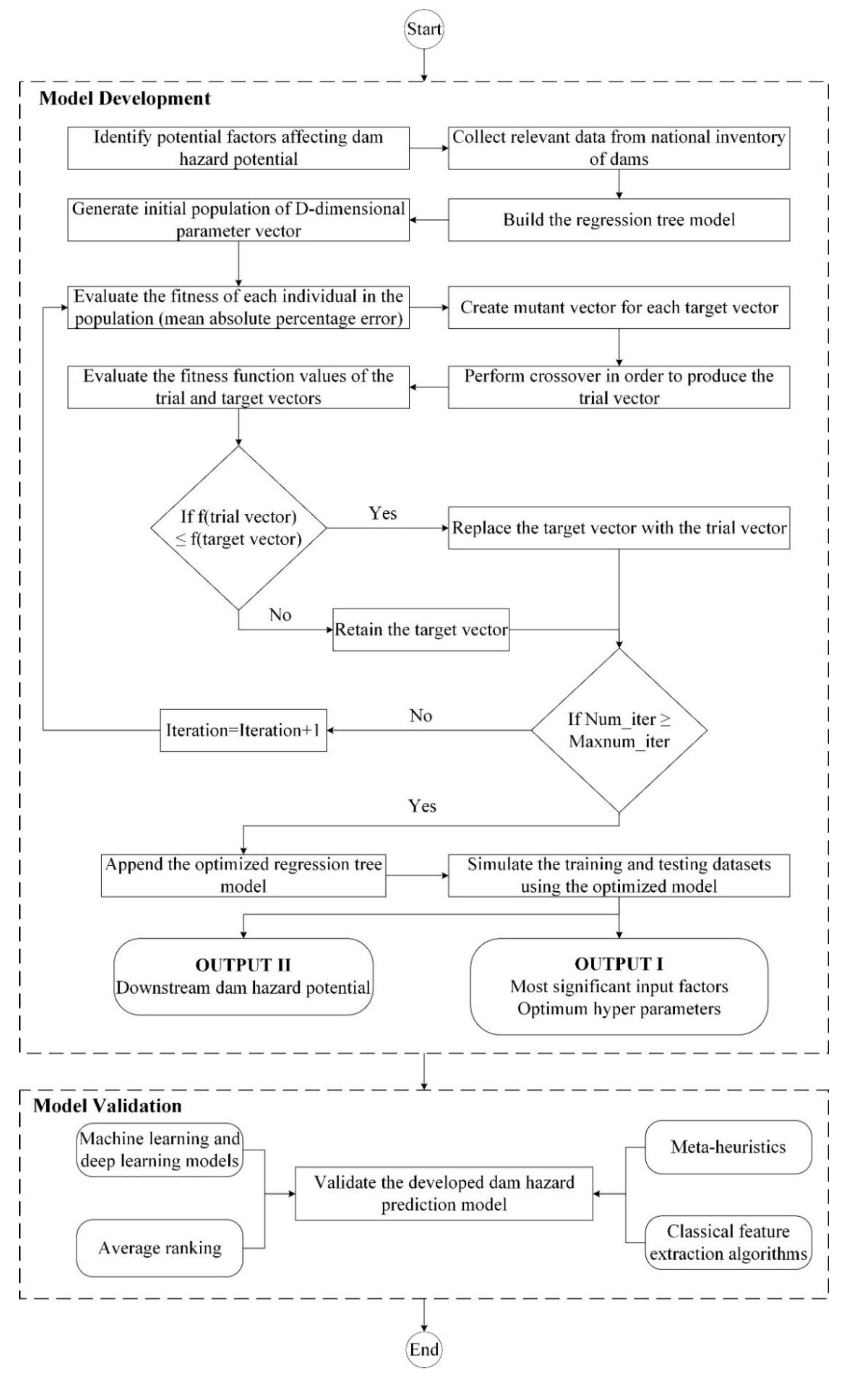
3. Research Framework

The paramount objective of this research paper was to establish an integrated data-driven model for the fast and efficient prediction of dam hazard potential. The framework of the developed dam hazard potential model is displayed in Figure 1. It is composed of two fundamental components, namely model development and model validation. Several standards, guidelines and manuals were reviewed to identify the input factors affecting dam hazard potential [33,34,35,36]. The dataset used in this research paper was retrieved from the national inventory of dams that is maintained and published by the United States Army Corps of Engineers (USACE) and the Association of State Dam Safety Officials (ASDSO) [2]. The congress authorized USACE to create a database for the inventory of dams in the United States and its territories in the 1970s under the national dam inspection act (public law 92–367) [2]. In this regard, the first inventory of dams was published in 1975 and the national inventory of dams was transformed into a web-based platform in the 1990s [2]. Table 1 records a list of 22 identified input factors that could affect dam hazard potential, alongside their descriptions. These input features encompass age, distance to nearest city/town, primary dam type, core type, foundation type, dam height, structural height, hydraulic height, NID height, dam length, dam volume, maximum storage, normal storage, NID storage, surface area, drainage area, maximum discharge, spillway type, spillway width, number of locks, length of locks, and width locks. The output is the downstream dam hazard potential, and it is classified to either: low, significant, or high, based on the consequences of the dams’ failure or misoperation (see Table 2).
The first component of the research framework is the model development. In it, an integrated differential evolution-based regression tree model is proposed to predict the downstream dam hazard potential. In the last decade, meta-heuristics suggested a higher competency could be achieved by boosting the search behavior of machine learning algorithms in diverse civil engineering applications such as damage detection in bridges [37], analysis of soil structure interaction [38], forecasting of annual rainfall [39], and the modeling of shield performance during tunneling [40]. Hence, the developed data-driven intelligent model exploits the use of the differential evolution algorithm for the following purposes:
  • Identifying the optimum subset of influential spatial features that significantly implicate downstream dam hazard potential;
  • Amplifying the prediction accuracies of regression tree through the automated optimization of its hyper parameters.
Regression tree is a variant of decision tree to simulate real-valued functions, instead of being utilized for classification purposes. Regression tree is constructed through the binary recursive partitioning process, which is an iterative process of splitting the data into homogenous partitions, and then the process is iterated to the branches until each node becomes a terminal node. The terminal node includes the predicted output value [41]. Regression tree is simple to implement, easy to understand, based fast data-driven learning, and is insensitive to outliers [42,43,44]. The differential evolution algorithm is selected for the feature selection and performance augmentation of regression trees owing to its simple structure, fast convergence speed, easy implementation, few control parameters, and robustness [45,46,47]. In addition, it has been successfully implemented by several scholars in solving complex optimization problems in several fields, such as time-cost tradeoff of construction projects [48], planning of public lighting installations [49], design of reinforced concrete foundations [50], and the arrangement of reinforcement layout of bridges [51]. The training process of the regression tree model is performed according to a single-objective optimization function which minimizes mean absolute percentage error of the predicted dam hazard potential. In this regard, the learning process of the regression tree model is iterated until the desired number of iterations set in the differential evolution algorithm is reached. There are two types of output in the first component. In this context, the first output is the optimum hyper parameters of the optimized regression tree model. The second is the predicted training and testing datasets using the optimized regression tree model.
The second component of the developed research framework aims at validating the developed differential evolution-based regression tree model, capitalizing on four folds of comparisons. In the first fold, the developed DE REGT model is compared against widely acknowledged machine learning and deep learning models to test its prediction accuracies. These models encompass long short-term memory ( LSTMs ) networks, deep convolutional neural networks ( DCNNs ), Gaussian process regression ( GPR ), cascade forward neural networks ( CFNNs ), feedforward neural networks ( FFNNs ), Elman neural networks ( ENNs ), bagged tree ( BAGTR ), boosted tree ( BOSTR ), and support vector machines ( SVMs ). The comparative analysis is undertaken using six performance evaluation metrics, namely mean absolute percentage error, relative absolute error, mean absolute error, root squared error, root mean squared error, and Nash–Sutcliffe efficiency. The second fold is designated to establish a consolidated ranking of the tackled data-driven intelligent models, as per their scores across the six-performance metrics. The third fold seeks to verify the use of the differential evolution algorithm for optimizing regression tree by comparison with some highly recognized population-based meta-heuristics involving particle swarm optimization ( PSO ), ant colony optimization ( ACO ), invasive weed optimization ( IWO ), teaching learning-based optimization ( TLBO ), grey wolf optimization ( GWO ), grasshopper optimization ( GO ), moth-flame optimization ( MFO ), ant lion optimization ( ALO ), the dragon fly algorithm ( DA ), and multi-verse optimization ( MVO ). The fourth component is used to test the applicability of using a differential evolution algorithm for feature extraction by comparing it with neighborhood component analysis ( NCA ) [52] and the ReliefF algorithm [53,54].

4. Model Development

This section describes the procedures of the differential evolution algorithm and the automated training mechanism of regression tree.

4.1. Differential Evolution

Differential evolution is a population-based search meta-heuristic algorithm that was proposed by Storn and Prince [55] to solve non-linear, non-differentiable, and multi-modal optimization problems. It uses similar operators to the genetic algorithm such as the initial generation of population, mutation, crossover, and selection. The main difference is that differential evolution capitalizes on mutation, while the genetic algorithm uses crossover [56,57]. The basic steps of the differential evolution algorithm as follows [55]:
The first step is to generate randomly generated solutions of N P size in a D-dimensional search space between the lower and upper bounds of the decision parameters. The initial population is generated randomly using Equation (1):
X i , g = L B + r × ( U B L B )  
where, X i , g refers to the individual of a population, and current generation, respectively. U B and L B are the upper and lower bounds of the design variables. r is a random number in the range of [0, 1].
The second step is the mutation, where a mutation vector is created for each target vector. The mutant vector is formed by adding the difference between two random vectors in the population to a third randomly selected vector. The mutant vector in the mutation operation is generated using Equation (2):
V i , g + 1 = X r 1 , g + F ( X r 2 , g X r 3 , g )   such   that   r 1 r 2   r 3
where, r 1 , r 2 , and r 3 are three randomly selected indices which are between 1 and N P and not equal to i . F is a mutation scale, and it is a real number in the range of [0, 1] that controls the amplification of differential variations.
The third step is the crossover, which aims at improving the diversity of individuals in the population through exchanging the components between the mutant vector and the target vector. The trial vector is defined using Equation (3):
U j , i , g + 1 = { V j , i , g + 1   i f   C R r a n d j   X j , i , g ,   i f   C R < r a n d j    
where, U j , i , g + 1 is the trial vector, and j represents the index of the vector i . C R is the crossover probability rate. r a n d j is a random number in the range of [0, 1] which ensures that at least one component of the trial vector is copied from the target vector.
The fourth step is the selection, such that the trial vector is compared against the target vector based on the objective function value. In the case of minimization cost functions, if the objective function value of the trial vector is less than that of the target vector, then the trial vector is selected over the target vector to be in the next generation. Otherwise, the old target vector is retained. The selection process is represented using Equation (4):
X i , g + 1 = { U i , g ,   i f   f ( U i , g ) > f ( X i , g )   X i , g ,   i f   f ( U i , g ) > f ( X i , g )    
where, X i , g + 1 is the target vector in the next generation and f ( ) is the objective function. The operators of mutation, crossover and selection are applied within each generation until a desired number of generations is reached.

4.2. Automated Training of Regression Tree

The developed model adopts the use of the differential evolution algorithm to determine the optimum hyper parameters of regression tree, and to identify the most significant dam hazard factors. The solution structure of the differential evolution-based training mechanism is presented in Figure 2. The variable X i stands for the value of the decision variable, whereas i indicates the length of the decision variable. In this regard, the length of the optimization problem is 26, the first four are related to the hyper parameters of regression tree, and the remaining twenty-two are pertinent to the dam hazard factors. For the hyper paraments, the developed training mechanism optimizes the values of minimum parent size, minimum leaf size for each tree, maximum number of splits, and type of split predictor selection. The variable X i takes the form of an integer number ranging from 1 to 200 for minimum parent size, minimum leaf size, and maximum number of splits. In addition, the variable X i is an integer number which is curvature (1), interaction–curvature (2), or all splits (3) in the split predictor selection. As for the hazard factors, the variable X i is a binary number which is either “1”, which implies that the hazard factor is significant, or “0” which implies that the hazard factor is not significant. The training process of regression tree is performed based on a single-objective optimization problem which minimizes the mean absolute percentage error of downstream dam hazard potential, as shown in Equation (5):
M A P E T = 100 T × t = 1 T | P T t A T t | A T t    
where, M A P E T is the mean absolute percentage error of the predicted dam hazard potential in the training dataset, T is the total number of instances in the training dataset, and P T t and A T t refer to the predicted dam hazard potential and actual dam hazard potential in the training dataset, respectively.

5. Performance Evaluation Metrics

The present research study accommodates the use of the performance metrics of mean absolute percentage error, relative absolute error, mean absolute error, root squared error, root mean squared error and Nash–Sutcliffe efficiency to assess the training and testing accuracies of the developed dam hazard potential prediction model against other models. These performance evaluation criteria can be mathematically calculated using Equations (6)–(11) [58,59,60,61]:
M A P E = 100 k × i = 1 K | P i O i | O i    
R A E = i = 1 K | ( A i P i ) |   i = 1 K | ( A i A i ) |    
A E = 1 K i = 1 K | ( A i P i ) |    
R S E = i = 1 K ( A i P i ) 2   i = 1 K ( A i A ¯ ) 2    
R M S E = 1 K i = 1 K ( A i P i ) 2    
N S E = 1 [ i = 1 K ( P i A i ) 2 i = 1 K ( A i A ¯ ) 2 ]  
where, A i and P i are the actual and predicted dam hazard potential, A ¯ is the mean of actual dam hazard potential, and K is the number of available observations of dams. The model with smaller values of mean absolute percentage error, relative absolute error, mean absolute error, root squared error, root mean squared error, and larger value of Nash–Sutcliffe efficiency is selected as a better model for simulating dam hazard potential.

6. Model Implementation

The validation process of the developed intelligent dam hazard potential models was undertaken using the 2020 national inventory of dams. After removing the missing observations, a dataset of 2016 and 504 dams were used for training and testing the data-driven models. The optimum hyper parameters of the conventional machine learning and deep learning were calibrated based on trial-and-error approach. The LSTM was implemented using 200 hidden units, a dam optimizer, and an initial learning rate of 5 × 10⁻³. The DCNN was composed of two convolutional layers; whereas the first one utilized 16 filters of size 2 × 2, the second utilized 16 filters of size 5 × 5. The first layer was followed by a batch normalization layer and a then a rectified linear unit function. The second convolutional layer was followed by a fully connected layer of 200 neurons. The initial learning rate and minimum batch size was set to 1 × 10⁻⁴ and 50, respectively. The kernel function in the GPR was squared exponential, and the hidden layer size was 10 in the CFNN . As for the FFNN , the numbers of hidden layers and numbers of hidden neurons were set to 6 and 2, respectively. The learning rate and momentum rate were assumed as 1 × 10⁻³ and 0.8, respectively. With regards to ENN , the numbers of hidden layers and context layers were four, and numbers of hidden neurons and context neurons were two. In the BAGTR , the minimum leaf size and learning rate were 8 and 0.1, respectively, and the minimum leaf size was 8 in the BOSTR . SVM was applied using coarse Gaussian kernel function.
In the developed DE REGT model, the population size and maximum number of iterations were assumed as 50 and 400, respectively. The crossover probability rate was assumed 0.2, and mutation scaling factor was assumed to follow a normal distribution between 0.2 and 0.8. Figure 3 displays the convergence behavior of the developed DE REGT model in predicting dam hazard potential. It was found that the developed DE REGT model converged to mean absolute percentage error of 7.42% at iteration 78. In the developed DE REGT model, the significant factors affecting downstream dam hazard potential involved: age, distance to nearest city/town, dam height, hydraulic height, structural height, NID height, dam length, dam volume, maximum storage, normal storage, NID storage, drainage area, maximum discharge, spillway type, spillway width, length of locks, and width of locks. In addition, the architecture of the optimized regression tree was composed of minimum parent size, minimum leaf size, and maximum number of splits of 5, 1 and 200, respectively, and all splits were of the optimum split predictor selection. Figure 4 and Figure 5 display illustrations of the prediction performances of the feedforward neural network, developed DE REGT model, Elman neural network, and support vector machines. In this regard, the predicted and actual hazard potential of twenty observations from the testing dataset were plotted. It can be observed that the developed DE REGT model managed to produce the predicted values of hazard potential that were very close and reasonably matched to the actual ones. However, the feedforward neural network, Elman neural network, and support vector machines failed to provide satisfactory agreement with the actual values of hazard potential, generating highly deviated values from them.
Figure 6 and Figure 7 demonstrate error histograms with 20 bins for the feedforward neural network, developed DE REGT model, Elman neural network, and support vector machines. The error included in these histograms was the absolute difference between the actual and predicted values of dam hazard potential, and the yellow vertical line denotes the zero error. It was noticed that most of the errors in the developed DE REGT model sustained an error of 0.05. In the feedforward neural network, the largest fraction of the errors ranged between 0.055 and 1.815. With regards to the Elman neural network, most of the errors varied between 0.051 and 1.785. The majority of the errors in the support vector machines fell between 0.054 and 0.821. Table 3 reports the prediction performance comparison results, where MAPE , RAE , MAE , RSE , RMSE and NSE can be found. It can be noticed that the developed DE REGT model was able to accomplish the highest prediction accuracies with an MAPE , RAE , MAE , RSE , RMSE and NSE of 9.62%, 0.27, 0.17, 0.31, 0.41 and 0.74, respectively. BOSTR yielded good prediction results, and the values of MAPE , RAE , MAE , RSE , RMSE and NSE were equal to 19.55%, 0.49, 0.32, 0.42, 0.48 and 0.64, respectively. However, CFNN provided the highest prediction error, such that MAPE , RAE , MAE , RSE , RMSE and NSE were 35.89%, 0.92, 0.6, 21.4, 3.44 and −17.1, respectively.
Table 4 records the ranking results according to the average ranking algorithm. It can be seen that the developed DE REGT model outranked the remainder of the data-driven intelligent models. Boosted tree and bagged tree were ranked in the second and third places, respectively. The deep convolutional neural network and the cascade forward neural network obtained the ninth and tenth rankings, respectively. It was also inferred that the developed DE REGT model, boosted tree, and bagged tree sustained a robust ranking across the six performance indicators. Furthermore, support vector machines experienced explicit variations in ranking across the performance indicators.
Figure 8 shows the convergence curves of the meta-heuristic-based regression tree models. The population size and number of iterations were set to 40 and 500, respectively, to ensure fair comparison between the meta-heuristics. The cognitive learning and social parameter were assumed as two in the particle swarm optimization algorithm. In the ant colony optimization algorithm, the intensification factor and sample size were equal to 0.5 and 40, respectively. As for the invasive weed optimization algorithm, the initial and final values of standard deviation were 0.5 and 0.001, respectively. In addition, the minimum and maximum number of seeds were 0 and 5, respectively. The motion vector in the grey wolf optimization were assumed to be linearly decreasing from two to zero. The minimum and maximum values of the deceleration of grasshoppers in the grasshopper optimization algorithm were equal to 0.00004 and 1, respectively. In the moth-flame optimization algorithm, the logarithmic spial motion constant was 1 and the convergence constant was assumed to be decreasing linearly from −1 to −2. The levy’s flight constant was assumed as 1.5 in the dragonfly algorithm. It can be viewed that the developed DE REGT model accomplished the lowest value of MAPE (7.42%). MFO REGT provided the second lowest MAPE (7.43%) followed by GWO REGT which achieved the third lowest MAPE (7.5%). On the other hand, IWO REGT had the highest value of MAPE (17.77%), and GO REGT yielded the second highest MAPE (9.97%).
Table 5 shows performance comparison assessment of the meta-heuristic-based regression tree models. It was perceived that the developed DE REGT model produced higher prediction accuracies than other meta-heuristic-based regression tree models. It was also inferred that ACO REGT , TLBO REGT , and MFO REGT accomplished acceptable prediction errors. In this regard, ACO REGT -sustained MAPE , RAE , MAE , RSE , RMSE , and NSE were 9.95%, 0.28, 0.18, 0.36, 0.45, and 0.7, respectively. In addition to that, both ACO REGT and MFO REGT achieved MAPE , RAE , MAE , RSE , RMSE , and NSE values of 10.56%, 0.29, 0.19, 0.32, 0.42, and 0.73, respectively. On the contrary, IWO REGT failed to accurately predict the downstream dam hazard potential, obtaining MAPE , RAE , MAE , RSE , RMSE , and NSE of 20.12%, 0.5, 0.33, 0.55, 0.55, and 0.54, respectively.
Table 6 presents a comparative analysis between the feature extraction algorithms for predicting downstream dam hazard potential. In it, the developed DE REGT model was validated against NCA REGT which used neighborhood component analysis for feature extraction and regression tree for prediction, and against ReliefF REGT which used ReliefF algorithm for feature extraction and regression tree for prediction. According to neighborhood component analysis, the significant subset of features encompassed dam length, dam volume, maximum storage, normal storage, NID storage, and maximum discharge. The most influential input factors as per the ReliefF algorithm included age, core type, foundation type, and dam length. Results illustrated that the developed DE REGT outperformed NCA REGT and ReliefF REGT across the six performance indicators. Moreover, NCA REGT yielded a lower prediction error than ReliefF REGT attaining MAPE , RAE , MAE , RSE , RMSE , and NSE of 16.09%, 0.41, 0.27, 0.46, 0.51, and 0.61, respectively. This evinces that using differential evolution could serve as a better feature extractor in analyzing dam hazard potential factors than neighborhood component analysis and ReliefF algorithms.
A sensitivity analysis was carried out to measure the extent of the implication of each input parameter on the downstream dam hazard potential. The sensitivity analysis was conducted for the developed DE–REGT model because it yielded the highest prediction accuracies. In the sensitivity analysis, a base control scenario was generated based on taking the average of the continuous variables, and the most frequent observation (mode) in the case of discrete categorical variables. Each input parameter was varied one at a time by increments ranging from its minimum to maximum values in the dam dataset, while the values of the remaining input parameters were fixed. In addition, this procedure was iterated for all input parameters. Figure 9 and Figure 10 show the impacts of the variations in age, dam height, NID height, and dam volume. It can be seen that the dam hazard potential increased as ages and dam height increased. In addition, NID height and dam volume were directly proportional to dam hazard potential. It can be noticed that dam hazard potential was more sensitive to age than dam height, NID height, and dam volume. Furthermore, NID height and dam volume exhibit a closer degree of sensitivity on downstream dam hazard potential. Table 7 reports the absolute difference between the maximum and minimum dam hazard potential for each input parameter. Results demonstrated NID storage with the greatest absolute difference (absolute difference = 0.4) followed by age (absolute difference = 0.33) and then hydraulic height (absolute difference = 0.28). On the other hand, primary dam type, core type, foundation type, spillway width, number of locks, length of locks, and width locks (absolute difference = 0) exhibited the least impact on downstream dam hazard potential.
Table 8 reports the training and testing times of the data-driven models for predicting dam hazard potential. It was found that the developed DE REGT model sustained the longest training time of 1775.3 s. This can be attributed to the ability of the developed model to optimize the influential factors affecting dam hazard potential and the hyper parameters of regression tree. LSTM (111.1 s) had the second longest training time while DCNN (95.2 s) was ranked in third place. On the other hand, GPR (11.2 s) and CFNN (10.6 s) had the shortest training times. As for the testing time, almost all of the data-driven models exhibited the same testing times that ranged from 0.05 s to 0.23 s, while LSTM had a longer testing time of 0.75 s than the remainder of the data-driven models.

7. Conclusions

A substantial number of dams registered in the national inventory of dams have high hazard potential ratings, and there are growing numbers of deficient dams in the United States. Hence, this research paper contributes to the body of relevant knowledge by presenting an intelligent data-driven model for the timely and efficient prediction of downstream dam hazard potential. The developed model was conceptualized on the amalgamation of differential evolution algorithm and regression tree, while differential evolution was deployed for feature selection, and boosting the prediction capabilities of regression tree through optimizing its main hyper parameters. The comparison results showed that the developed DE REGT model produced significantly lower prediction errors than the remaining machine learning and deep learning models. It generated MAPE , RAE , MAE , RSE , RMSE , and NSE values of 9.62%, 0.27, 0.17, 0.31, 0.41, and 0.74, respectively. Boosted tree gave a comparatively lower prediction error with MAPE , RAE , MAE , RSE , RMSE , and NSE of 19.5%, 0.49, 0.32, 0.42, 0.48, and 0.64, respectively. On the other contrary, cascade forward neural network was unable to accurately predict the dam hazard potential, providing the highest prediction error with values of MAPE , RAE , MAE , RSE , RMSE , and NSE corresponding to 35.89%, 0.92, 0.6, 21.4, 3.44, and −17.1, respectively. In this regard, the developed DE REGT model performed better than FFNN , ENN , SVM , and LSTM by 75.19%, 72.29% 103.11%, and 63.86%, respectively. The average ranking algorithm revealed that the developed DE REGT model was able to achieve higher rank and a more robust performance based on its scores in the evaluation metrics. Moreover, boosted tree, bagged tree and long short-term memory network were ranked in the second, third and fourth places, respectively. On the other hand, CFNN and DCNN achieved lower ranking among the investigated data-driven models, failing to appropriately predict the dam hazard potential. In addition, it was observed that the performances of support vector machines and deep convolutional neural networks were highly fluctuated across the prediction evaluation metrics achieving standard deviation of rankings of 1.49 and 1, respectively.
Comparison assessment results also signified the efficacy of the differential evolution algorithm in the hyper parameter optimization of regression tree, and the developed DE REGT was able to perform better than the other ten meta-heuristic-based regression tree models. It managed to improve the prediction accuracies by 9.14%, 6.96%, 5.76%, and 42.35% with reference to PSO REGT , TLBO REGT , ACO REGT , and IWO REGT , respectively. Conversely, the invasive weed optimization algorithm was found as an inadequate tool to optimize the hyper parameters of regression tree, such that IWO REGT produced MAPE , RAE , MAE , RSE , RMSE and NSE corresponding to 20.12%, 0.5, 0.33, 0.55, 0.55 and 0.54, respectively. The evaluation of feature extraction algorithms manifested the superiority of differential evolution over neighborhood component analysis and ReliefF , whereas the developed DE REGT model succeeded in lessening their prediction error by 30.85% and 54.35%, respectively. The above performance comparisons illustrate the success of the differential evolution algorithm to be used for the hyper parameter optimization of regression tree and feature extraction. Comparisons of running times illustrated that the DE REGT required the longest training time. Moreover, the long short-term memory network yielded the longest testing time among the data-driven models. It is expected that the developed data-driven model could provide asset managers with straightforward and useful guidance tools to explore the magnitude of consequences of dam failure or misoperation, which could improve the maintenance management of prioritization actions and maximize the effectiveness of risk reduction and safety evaluation measures. This research paper can be extended in the future in three directions. First, the framework could include moving vehicles and dam leakage, and go on to study their impact on downstream dam hazard potential. Second, the simulation output of the data-driven model could be explored further by considering the probability of hazard occurrence. Third, quantitative tools could be used to evaluate downstream dam hazard potential and to link this with the structural capacity of dams.

Author Contributions

Conceptualization, E.M.A. and A.A.-S.; methodology, E.M.A. and A.A.-S.; formal analysis E.M.A., A.A.-S., G.A. and N.E.; data curation, E.M.A., A.A.-S., G.A. and N.E.; investigation, E.M.A., A.A.-S., G.A. and N.E.; writing—original draft preparation, E.M.A., A.A.-S., G.A. and N.E.; writing—review and editing, E.M.A., A.A.-S., G.A. and N.E. All authors have read and agreed to the published version of the manuscript.

Funding

This research received no external funding.

Institutional Review Board Statement

Not applicable.

Informed Consent Statement

Not applicable.

Data Availability Statement

Some or all data, models, or code that support the findings of this study are available from the corresponding author upon reasonable request.

Conflicts of Interest

The authors declare no conflict of interest.

References

  1. Shi, H.; Chen, J.; Liu, S.; Sivakumar, B. The Role of Large Dams in Promoting Economic Development under the Pressure of Population Growth. Sustainability 2019, 11, 2965. [Google Scholar] [CrossRef] [Green Version]
  2. United States Army Corps of Engineers. National Inventory of Dams. 2020. Available online: https://nid.usace.army.mil/#/ (accessed on 26 January 2022).
  3. American Society of Civil Engineers. Report Card for American Infrastructure. 2021. Available online: https://infrastructurereportcard.org/ (accessed on 26 January 2022).
  4. Mehta, A.M.; Weeks, C.S.; Tyquin, E. Towards preparedness for dam failure: An evidence base for risk communication for downstream communities. Int. J. Disaster Risk Reduct. 2020, 50, 101820. [Google Scholar] [CrossRef]
  5. Koppe, J.C. Lessons Learned from the Two Major Tailings Dam Accidents in Brazil. Mine Water Environ. 2020, 40, 166–173. [Google Scholar] [CrossRef]
  6. Perera, D.; North, T. The Socio-Economic Impacts of Aged-Dam Removal: A Review. J. Geosci. Environ. Prot. 2021, 9, 62–78. [Google Scholar] [CrossRef]
  7. Vahedifard, F.; Madani, K.; AghaKouchak, A.; Thota, S.K. Are we ready for more dam removals in the United States? Environ. Res. Infrastruct. Sustain. 2021, 1, 1–6. [Google Scholar] [CrossRef]
  8. Güven, A.; Aydemir, A. Dam Safety. In Risk Assessment of Dams; Springer: Berlin/Heidelberg, Germany, 2020; pp. 15–49. [Google Scholar]
  9. Pisaniello, J.D.; Dam, T.T.; Tingey-Holyoak, J.L. International small dam safety assurance policy benchmarks to avoid dam failure flood disasters in developing countries. J. Hydrol. 2015, 531, 1141–1153. [Google Scholar] [CrossRef]
  10. Adamo, N.; Al-Ansari, N.; Sissakian, V.; Laue, J.; Knutsson, S. Dam Safety and Dams Hazards. J. Earth Sci. Geotech. Eng. 2020, 10, 23–40. [Google Scholar]
  11. Burk, R.A.; Kallberg, J. Cyber Defense as a part of Hazard Mitigation: Comparing High Hazard Potential Dam Safety Programs in the United States and Sweden. J. Homel. Secur. Emerg. Manag. 2016, 13, 77–94. [Google Scholar] [CrossRef]
  12. American Society of Civil Engineers. Senate Appropriators Fund High Hazard Dam Rehab Program. 2020. Available online: https://infrastructurereportcard.org/senate-appropriators-fund-high-hazard-dam-rehab-program/ (accessed on 24 January 2022).
  13. Assad, A.; Bouferguene, A. Data Mining Algorithms for Water Main Condition Prediction—Comparative Analysis. J. Water Resour. Plan. Manage 2022, 148, 04021101. [Google Scholar] [CrossRef]
  14. Li, X.; Khademi, F.; Liu, Y.; Akbari, M.; Wang, C.; Bond, P.L.; Keller, J.; Jiang, G. Evaluation of data-driven models for predicting the service life of concrete sewer pipes subjected to corrosion. J. Environ. Manag. 2019, 234, 431–439. [Google Scholar] [CrossRef] [PubMed]
  15. Choi, S.; Do, M. Development of the Road Pavement Deterioration Model Based on the Deep Learning Method. Electronics 2019, 9, 3. [Google Scholar] [CrossRef] [Green Version]
  16. Kim, K.; Nam, M.; Hwang, H.; Ann, K. Prediction of Remaining Life for Bridge Decks Considering Deterioration Factors and Propose of Prioritization Process for Bridge Deck Maintenance. Sustainability 2020, 12, 10625. [Google Scholar] [CrossRef]
  17. Hassan, S.; Elwakil, E. Operational Based Stochastic Cluster Regression-Based Modeling for Predicting Condition Rating of Highway Tunnels. Can. J. Civ. Eng. 2021, 48, 77–94. [Google Scholar] [CrossRef]
  18. Xue, D.; Duan, Y.; Meng, W. Computer Intelligent Comprehensive Rapid Risk Assessment System of Barrier Dam by Fuzzy Analytic Hierarchy Process and Big Data. J. Phys. Conf. Ser. 2021, 2083, 042046. [Google Scholar] [CrossRef]
  19. Daud, N.M.; Hassan, S.H.; Akbar, N.A.; Bakar, A.A.A.; Mohamad, N.A.S.; Manan, E.A.; Hamzah, A.F. Dam failure risk factor analysis using AHP method. IOP Conf. Ser. Earth Environ. Sci. 2021, 646, 012042. [Google Scholar] [CrossRef]
  20. Guetz, K.; Joyal, T.; Dickson, B.; Perry, D. Prioritizing dams for removal to advance restoration and conservation efforts in the western United States. Restor. Ecol. 2021, e13583. [Google Scholar] [CrossRef]
  21. Celik, E.; Gul, M. Hazard identification, risk assessment and control for dam construction safety using an integrated BWM and MARCOS approach under interval type-2 fuzzy sets environment. Autom. Constr. 2021, 127, 103699. [Google Scholar] [CrossRef]
  22. He, G.; Chai, J.; Qin, Y.; Xu, Z.; Li, S. Coupled Model of Variable Fuzzy Sets and the Analytic Hierarchy Process and its Application to the Social and Environmental Impact Evaluation of Dam Breaks. Water Resour. Manag. 2020, 34, 2677–2697. [Google Scholar] [CrossRef]
  23. Ribas, J.R.; Severo, J.C.R.; Guimarães, L.F.; Perpetuo, K.P.C. A fuzzy FMEA assessment of hydroelectric earth dam failure modes: A case study in Central Brazil. Energy Rep. 2021, 7, 4412–4424. [Google Scholar] [CrossRef]
  24. Lu, X.; Pei, L.; Chen, J.; Wu, Z.; Chen, C. Research and Application of a Seismic Damage Classification Method of Concrete Gravity Dams Using Displacement in the Crest. Appl. Sci. 2020, 10, 4134. [Google Scholar] [CrossRef]
  25. Li, Z.; Wu, Z.; Lu, X.; Zhou, J.; Chen, J.; Liu, L.; Pei, L. Efficient seismic risk analysis of gravity dams via screening of intensity measures and simulated non-parametric fragility curves. Soil Dyn. Earthq. Eng. 2021, 152, 107040. [Google Scholar] [CrossRef]
  26. Irinyemi, S.A.; Lombardi, D.; Ahmad, S.M. Correction to: Seismic risk analysis for large dams in West Coast basin, southern Ghana. J. Seism. 2022, 26, 117. [Google Scholar] [CrossRef]
  27. De Mello, A.R.; Barbosa, F.G.O.; Fonseca, M.L.; Smiderle, C.D. Concrete Dam Inspection with UAV Imagery and DCNN-based Object Detection. In Proceedings of the IEEE International Conference on Imaging Systems and Techniques (IST), New York, NY, USA, 24–26 August 2021; pp. 1–6. [Google Scholar]
  28. Feng, C.; Zhang, H.; Wang, H.; Wang, S.; Li, Y. Automatic Pixel-Level Crack Detection on Dam Surface Using Deep Convolutional Network. Sensors 2020, 20, 2069. [Google Scholar] [CrossRef] [PubMed] [Green Version]
  29. Yu, D.; Tang, L.; Ye, F.; Chen, C. A virtual geographic environment for dynamic simulation and analysis of tailings dam failure. Int. J. Digit. Earth 2021, 14, 1194–1212. [Google Scholar] [CrossRef]
  30. Hu, L.; Yang, X.; Li, Q.; Li, S. Numerical Simulation and Risk Assessment of Cascade Reservoir Dam-Break. Water 2020, 12, 1730. [Google Scholar] [CrossRef]
  31. Huang, J.; Sun, W.; Huang, L. Deep neural networks compression learning based on multiobjective evolutionary algorithms. Neurocomputing 2019, 378, 260–269. [Google Scholar] [CrossRef]
  32. Xie, H.; Zhang, L.; Lim, C.P. Evolving CNN-LSTM Models for Time Series Prediction Using Enhanced Grey Wolf Optimizer. IEEE Access 2020, 8, 161519–161541. [Google Scholar] [CrossRef]
  33. Federal Emergency Management Agency. The National Dam Safety Program; Federal Emergency Management Agency: Washington, DC, USA, 2016. [Google Scholar]
  34. United States Department of Homeland Security. Dams Sector-Specific Plan—An Annex to the National Infrastructure Protection Plan; United States Department of Homeland Security: Washington, DC, USA, 2010. [Google Scholar]
  35. United States Army Corps of Engineers. National Inventory of Dams: Methodology; United States Army Corps of Engineers: Norfolk, VA, USA, 2008. [Google Scholar]
  36. Federal Emergency Management Agency. Federal Guidelines for Dam Safety: Hazard Potential Classification System for Dams; U.S. Department of Homeland Security: Washington, DC, USA, 2004.
  37. Huang, M.; Lei, Y.; Li, X.; Gu, J. Damage Identification of Bridge Structures Considering Temperature Variations-Based SVM and MFO. J. Aerosp. Eng. 2021, 34, 04020113. [Google Scholar] [CrossRef]
  38. Milajerdi, B.M.; Behnamfar, F. Soil-structure interaction analysis using neural networks optimised by genetic algorithm. Geomech. Geoengin. 2021, 1–19. [Google Scholar] [CrossRef]
  39. Diop, L.; Samadianfard, S.; Bodian, A.; Yaseen, Z.M.; Ghorbani, M.A.; Salimi, H. Annual Rainfall Forecasting Using Hybrid Artificial Intelligence Model: Integration of Multilayer Perceptron with Whale Optimization Algorithm. Water Resour. Manage. 2020, 34, 733–746. [Google Scholar] [CrossRef]
  40. Elbaz, K.; Shen, S.-L.; Sun, W.-J.; Yin, Z.-Y.; Zhou, A. Prediction Model of Shield Performance During Tunneling via Incorporating Improved Particle Swarm Optimization Into ANFIS. IEEE Access 2020, 8, 39659–39671. [Google Scholar] [CrossRef]
  41. Breiman, L.; Friedman, J.H.; Olshen, R.A.; Stone, C.J. Classification and Regression Trees; CRC Press: Boca Raton, FL, USA, 1984. [Google Scholar]
  42. Pandit, R.K.; Infield, D. SCADA based nonparametric models for condition monitoring of a wind turbine. J. Eng. 2019, 2019, 4723–4727. [Google Scholar] [CrossRef]
  43. Crespo-Peremarch, P.; Ruiz, L.; Balaguer-Beser, A. A comparative study of regression methods to predict forest structure and canopy fuel variables from LiDAR full-waveform data. Revista de Teledetección 2016, 45, 27–40. [Google Scholar] [CrossRef] [Green Version]
  44. Aertsen, W.; Kint, V.; van Orshoven, J.; Özkan, K.; Muys, B. Comparison and ranking of different modelling techniques for prediction of site index in Mediterranean mountain forests. Ecol. Model. 2010, 221, 1119–1130. [Google Scholar] [CrossRef]
  45. Sun, G.; Li, C.; Deng, L. An adaptive regeneration framework based on search space adjustment for differential evolution. Neural Comput. Appl. 2021, 33, 9503–9519. [Google Scholar] [CrossRef]
  46. Sun, X.; Lin, K.; Jiao, P.; Lu, H. Signal Timing Optimization Model Based on Bus Priority. Information 2020, 11, 325. [Google Scholar] [CrossRef]
  47. Gao, S.; Wang, K.; Tao, S.; Jin, T.; Dai, H.; Cheng, J. A state-of-the-art differential evolution algorithm for parameter estimation of solar photovoltaic models. Energy Convers. Manag. 2021, 230, 113784. [Google Scholar] [CrossRef]
  48. Luong, D.-L.; Tran, D.-H.; Nguyen, P.T. Optimizing multi-mode time-cost-quality trade-off of construction project using opposition multiple objective difference evolution. Int. J. Constr. Manag. 2018, 21, 271–283. [Google Scholar] [CrossRef]
  49. Rabaza, O.; Gómez-Lorente, D.; Pozo, A.M.; Pérez-Ocón, F. Application of a Differential Evolution Algorithm in the Design of Public Lighting Installations Maximizing Energy Efficiency. Leukos 2019, 16, 217–227. [Google Scholar] [CrossRef]
  50. Kamal, M.; Inel, M. Optimum Design of Reinforced Concrete Continuous Foundation Using Differential Evolution Algorithm. Arab. J. Sci. Eng. 2019, 44, 8401–8415. [Google Scholar] [CrossRef]
  51. Chikahiro, Y.; Ario, I.; Pawlowski, P.; Graczykowski, C.; Holnicki-Szulc, J. Optimization of reinforcement layout of scissor-type bridge using differential evolution algorithm. Comput. Civ. Infrastruct. Eng. 2018, 34, 523–538. [Google Scholar] [CrossRef]
  52. Yang, W.; Wang, K.; Zuo, W. Neighborhood Component Feature Selection for High-Dimensional Data. J. Comput. 2012, 7, 161–168. [Google Scholar] [CrossRef]
  53. Kira, K.; Rendell, L.A. The Feature Selection Problem: Traditional Methods and a New Algorithm. In Proceedings of the Tenth National Conference on Artificial Intelligence (AAAI-92), San Jose, CA, USA, 12–16 July 1992; pp. 129–134. [Google Scholar]
  54. Robnik-Šikonja, M.; Kononenko, I. Theoretical and Empirical Analysis of ReliefF and RReliefF. Mach. Learn. 2003, 53, 23–69. [Google Scholar] [CrossRef] [Green Version]
  55. Storn, R.; Price, K. Differential Evolution—A simple and efficient adaptive scheme for global optimization over continuous spaces. J. Glob. Optim. 1997, 11, 341–359. [Google Scholar] [CrossRef]
  56. Tang, Z.; Hu, X.; Périaux, J. Multi-level Hybridized Optimization Methods Coupling Local Search Deterministic and Global Search Evolutionary Algorithms. Arch. Comput. Methods Eng. 2019, 27, 939–975. [Google Scholar] [CrossRef]
  57. Örkcü, H.H.; Aksoy, E.; Dogan, M.I. Estimating the parameters of 3-p Weibull distribution through differential evolution. Appl. Math. Comput. 2015, 251, 211–224. [Google Scholar] [CrossRef]
  58. Chen, L.; Yan, H.; Yan, J.; Wang, J.; Tao, T.; Xin, K.; Li, S.; Pu, Z.; Qiu, J. Short-term water demand forecast based on automatic feature extraction by one-dimensional convolution. J. Hydrol. 2022, 606, 127440. [Google Scholar] [CrossRef]
  59. Jalal, F.E.; Xu, Y.; Iqbal, M.; Javed, M.F.; Jamhiri, B. Predictive modeling of swell-strength of expansive soils using artificial intelligence approaches: ANN, ANFIS and GEP. J. Environ. Manag. 2021, 289, 112420. [Google Scholar] [CrossRef] [PubMed]
  60. Pandey, M.; Jamei, M.; Karbasi, M.; Ahmadianfar, I.; Chu, X. Prediction of Maximum Scour Depth near Spur Dikes in Uniform Bed Sediment Using Stacked Generalization Ensemble Tree-Based Frameworks. J. Irrig. Drain. Eng. 2021, 147, 04021050. [Google Scholar] [CrossRef]
  61. Muhsun, S.S.; Al-Madhhachi, A.S.T.; Al-Sharify, Z.T. Prediction and CFD Simulation of the Flow over a Curved Crump Weir Under Different Longitudinal Slopes. Int. J. Civ. Eng. 2020, 18, 1067–1076. [Google Scholar] [CrossRef]
Figure 1. Framework of the developed data-driven model for predicting dam hazard potential.
Sustainability 14 03013 g001
Figure 2. Representation of solution structure of the developed differential evolution-based training mechanism.
Sustainability 14 03013 g002
Figure 3. Convergence curve of the developed DE REGT model in predicting dam hazard potential.
Sustainability 14 03013 g003
Figure 4. Illustration of the prediction performances of the feedforward neural network and the developed DE REGT model. (a) Feedforward neural network. (b) Developed DE REGT model.
Sustainability 14 03013 g004
Figure 5. Illustration of the prediction performances of Elman neural network and support vector machines. (a) Elman neural network. (b) Support vector machines.
Sustainability 14 03013 g005
Figure 6. Error histograms of the feedforward neural network and the developed DE REGT model. (a) Feedforward neural network. (b) Developed DE REGT model.
Sustainability 14 03013 g006
Figure 7. Error histograms of Elman neural network and support vector machines. (a) Elman neural network. (b) Support vector machines.
Sustainability 14 03013 g007
Figure 8. Convergence curves of the meta-heuristic-based regression tree models.
Sustainability 14 03013 g008
Figure 9. Representations of the effect of age and height on downstream dam hazard potential. (a) dam age vs. hazard potential; (b) dam volume vs. hazard potential.
Sustainability 14 03013 g009
Figure 10. Representations of the effect of NID height and volume on downstream dam hazard potential. (a) NID height vs. hazard potential; (b) dam volume vs. hazard potential.
Sustainability 14 03013 g010
Table 1. Description of the prospective input variables affecting dam hazard potential [35].
Input VariableDescription
Age (years)Age in years since the construction of the dam was completed.
Distance to nearest city/town (miles)Distance from the dam to the nearest affected downstream village/town/city.
Primary dam typeType of dam can be either earth (1), rockfill (2), gravity (3), buttress (4), arch (5), multi-arch (6), roller-compacted concrete (7), concrete (8), masonry (9), stone (10), timber-crib (11), or other (12).
Core typeCore type can be either concrete (1), bituminous concrete (2), earth (3), metal (4), or plastic (5).
Foundation typeFoundation type can be either rock (1), soil (2), rock and soil (3), or other (4).
Dam height (feet)The vertical distance between the lowest point on the crest of the dam and the lowest point in the original streambed.
Hydraulic height (feet)The vertical distance between the maximum design water level and the lowest point in the original streambed.
Structural height (feet)The vertical distance between the lowest point of the excavated foundation to the top of the dam (parapet wall).
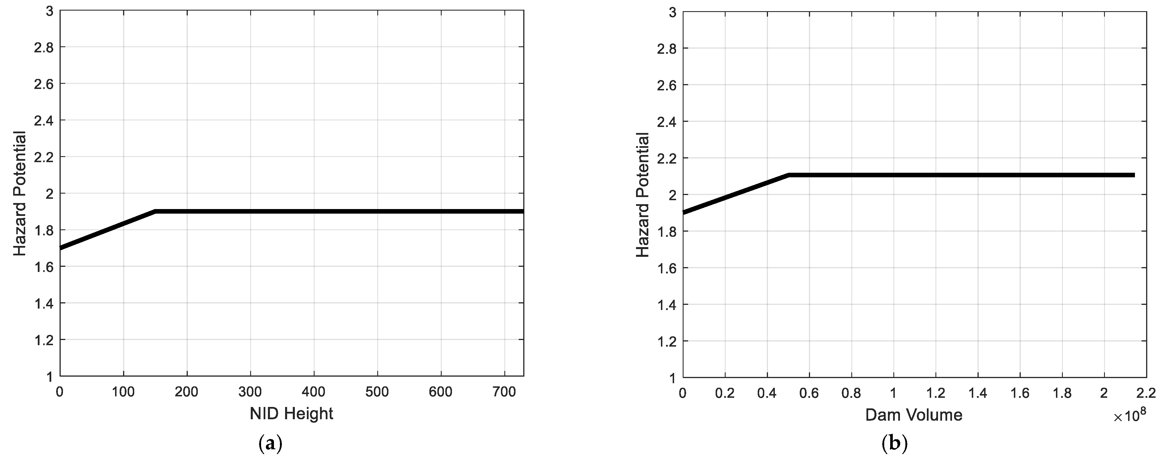
NID height (feet)The maximum value of the dam height, hydraulic height, or structural height.
Dam length (feet)Length along the top of the dam, which encompasses spillway, powerplant, navigation, fish pass, and lock.
Dam volume (cubic yard)The total number of cubic yards occupied by the materials used in the dam structure.
Maximum storage (acre-feet)The total storage space in a reservoir below the maximum attainable water surface elevation involving any surcharge storage.
Normal storage (acre-feet)The total storage space in a reservoir below the normal retention level involving dead and inactive storage and excluding any surcharge storage or flood control.
NID storageThe maximum value of the maximum storage and normal storage.
Surface area (acres)The surface area of the impoundment as the normal retention level.
Drainage area (square miles)The area that drains to a particular point on a stream or river.
Maximum discharge (cubic feet/second)The number of cubic feet per second that the spillway is able of discharging when the reservoir is at its maximum designed water surface elevation.
Spillway typeSpillway type can be controlled (1), uncontrolled (2), or none (3).
Spillway width (feet)The width available for discharge when the reservoir is at its maximum designed water surface elevation.
Number of locksNumber of existing navigation locks in the project.
Length of locks (feet)The length of the primary navigation lock.
Width of locks (feet)The width of the primary navigation lock.
Table 2. Description of the output downstream dam hazard potential and its categories [35].
Output VariableDescription
Downstream dam hazard potentialIndicates the potential hazard to the downstream area resulting from the failure or misoperation of the dam. It can be low (1), significant (2), or high (3).
Low hazard potential dams are those whose failure or misoperation results in no probable loss of human life and low economic and/or environmental losses.
Significant hazard potential dams are those whose failure or misoperation results in no probable loss of human life, but can result in economic loss, environmental damage, or disruption of lifeline facilities.
High hazard potential dams are those whose failure or misoperation could cause potential loss of human life, and can result in economic loss, environmental damage, or disruption of lifeline facilities.
Table 3. Performance comparison between data-driven models for predicting dam hazard potential.
Data-Driven ModelMAPERAEMAERSERMSENSE
LSTM 28.68%0.710.470.740.640.38
DCNN 31.80%1.130.742.041.06−0.72
GPR 31.03%0.730.480.750.650.36
CFNN 35.89%0.920.621.43.44−17.1
FFNN 34.57%0.80.520.820.670.3
ENN 32.12%0.780.510.80.670.32
BAGTR 22.89%0.60.390.620.590.48
BOSTR 19.50%0.490.320.420.480.64
SVM 24.90%0.750.490.970.730.18
DE REGT 9.62%0.270.170.310.410.74
Table 4. Mean and standard deviation of rankings of the data-driven models for predicting dam hazard potential.
Data-Driven ModelMean RankingStandard Deviation of RankingsFinal Ranking
LSTM 4.170.374
DCNN 919
GPR 5.170.375
CFNN 9.670.4710
FFNN 7.670.758
ENN 6.670.756
BAGTR 303
BOSTR 202
SVM 6.671.497
DE REGT 1.0001
Table 5. Performance comparison between the meta-heuristic-based regression tree models for predicting dam hazard potential.
Data-Driven ModelMAPERAEMAERSERMSENSE
DE REGT 9.62%0.270.170.310.410.74
PSO REGT 11.09%0.310.20.330.430.72
ACO REGT 10.56%0.290.190.320.420.73
IWO REGT 20.12%0.500.330.550.550.54
TLBO REGT 9.95%0.280.180.360.450.70
GWO REGT 12.39%0.330.220.410.480.65
GO REGT 11.36%0.300.20.330.430.72
MFO REGT 10.56%0.290.190.320.420.73
ALO REGT 11.44%0.310.20.340.430.71
DA REGT 12.34%0.330.210.380.460.68
MVO REGT 11.55%0.310.200.330.430.72
Table 6. Performance comparison between the feature extraction algorithms for predicting dam hazard potential.
Data-Driven ModelMAPERAEMAERSERMSENSE
DE REGT 9.62%0.270.170.310.410.74
NCA REGT 16.09%0.410.270.460.510.61
ReliefF REGT 24.88%0.640.420.650.60.45
Table 7. Summary of the results of sensitivity analysis for downstream dam hazard potential.
Input VariableAverageModeAbsolute Difference
Age54.80.33
Distance to nearest city/town 9.20.09
Primary dam typeEarth0
Core typeEarth0
Foundation typeSoil0
Dam height47.10.14
Hydraulic height45.20.28
Structural height540.08
NID height58.20.2
Dam length2895.50.06
Dam volume1,067,660.90.2
Maximum storage293,0200.04
Normal storage221,477.20.09
NID storage2932,61.30.4
Surface area11,1380.07
Drainage area3415.20.01
Maximum discharge40,264.90.23
Spillway typeUncontrolled0.07
Spillway width174.60
Number of locks00
Length of locks30.70
Width of locks4.60
Table 8. Training and testing times of data-driven models for predicting dam hazard potential.
Data-Driven ModelTraining Time (Seconds)Testing Time (Seconds)
LSTM 111.10.75
DCNN 95.20.23
GPR 11.20.12
CFNN 10.60.13
FFNN 12.50.13
ENN 18.80.45
BAGTR 13.50.07
BOSTR 13.80.05
SVM 17.50.07
DE REGT 1775.30.17
Publisher’s Note: MDPI stays neutral with regard to jurisdictional claims in published maps and institutional affiliations.

