A Stochastic Optimization Model for Sustainable Multimodal Transportation for Bioenergy Production

Abstract

While many previous studies have suggested well-defined procedures to find appropriate supply chains, a limited number of studies have been conducted with uncertain values relating to transportation costs. Most of these have included only limited detail on multimodal transportation, or have not considered economic, social, and environmental transportation cost factors together. The main purpose of this study is to suggest a multi-objective stochastic model for sustainable biomass transportation, and to identify the impact level of model selection on the transportation mode. It begins with a deterministic formulation of sustainable transportation, which is then modified to a stochastic problem with vectorization of cost parameters. Based on the model developed, we examined four uncertainty cases from a combination of annual capacity and average distance of biomass transportation. The experimental results provide more cost savings from multimodal transportation, which can be identified if we analyze transportation costs with stochastic modeling. Regarding short-distance plant cases, the study reveals that the impact of the utilization of stochastic methods is insignificant, as the costs savings from multimodal transportation is trivial. Other findings from the experiments show that multimodal transportation could provide cost savings in the economic cost factor, except in the case of low annual capacity and short average distance.

1. Introduction

While bioenergy has received increased attention as a potential replacement for fossil fuels in energy production, the share of US energy generated by biomass has remained the same over the last decade. This is because the implementation of bioenergy can increase only if it can be justified from an economic, environmental and social perspective. One of the critical aspects required to increase its usage is cost-effective transportation. Transportation is critical to bioenergy production, as the intrinsic characteristics of biomass cause transportation to account for a high proportion of costs in the overall biomass supply chain. This also makes transportation an important area of study in terms of the bioenergy supply chain.

Biomass transportation research commonly includes modeling approaches, both in the form of optimization and simulation. Optimization methods, sometimes called analytical tools, commonly use data processing through mathematical equations or algebraic expressions. Most optimization models have used a deterministic mathematical programming approach [1,2,3,4]. For example, Devlin and Talbot (2014) [3] used a linear programming approach to analyze transportation strategies for optimal woody biomass allocation to meet the co-firing targets of Ireland. Similarly, Sosa et al. (2015) [4] developed a linear programming model to analyze the optimal wood supply of short wood for the peat-based electricity sector that minimized harvesting, storage, chipping and transportation costs, while also considering competition with existing wood-based panel industries. Recently, stochastic programming models have been suggested to overcome these uncertainties [5,6,7]. For instance, Osmani and Zhang (2014) [5] proposed a stochastic programming model which sought to optimally balance supply from wind and biomass resources considering regional electricity demand and uncertainties in wind speed. While several other researchers have also chosen a mathematical programming approach to address uncertain parameters, most studies account for the energy price [5,8], market demand [9], and feedstock supply quantities [7] as uncertain parameters. A limited number of studies have been conducted with uncertain values relating to transportation costs. Kim et al. (2011) [10] have tried to figure out the impact of several uncertain parameters, including transportation cost, to reduce the design problem to a manageable size. However, they suggested a robustness and global sensitivity analysis using Monte Carlo simulation, rather than the stochastic optimization model. Thus, this study seeks to determine the impact on the complete transportation costs while considering uncertainty parameters.

When it comes to the mode of biomass transportation, most previous papers considered only a single mode of transport, the truck [11,12,13,14], as trucks are the dominant mode of biomass transportation. Rail transportation possesses unavoidable shortcomings due to limited accessibility and specific infrastructure needs, such as track, terminals, rail sidings, and transload facilities/equipment, but does become economically attractive with higher volumes and/or distances. Especially in the case of a large capacity bioenergy plant, interest in multimodal transportation using truck and rail may increase as well, since biomass utilization economics are sensitive to mobilization costs and hauling distances to markets [15]. Also, inclusion of external cost factors such as social and environmental costs escalate the share of rail shipments to minimize total sustainable transportation costs [16]. A study by Kumar et al. (2006) [17] also suggests the importance of multimodal transportation by determining the ranking of alternatives for biomass transportation systems while considering economic, social, environmental, and technical factors. The study found rail was the best alternative, followed by truck and pipeline for large capacity bioenergy production.

In this paper, the general integer linear/nonlinear programming models for a simple biomass transportation network for single and multimodal transportation scenarios is formulated. The main purposes of this study are to suggest the multi-objective stochastic model for sustainable biomass transportation system, and to identify the impact level of model selection (deterministic and stochastic) on a transportation mode (single and multimodal transportation). The study begins with a deterministic formulation of sustainable transportation which considers economic, social, and environmental cost factors. Then it is modified to a stochastic problem with vectorization of cost parameters. Four uncertainty scenarios are developed from different combinations of annual capacity and average distance of biomass transportation and then examined based on the developed stochastic model of biomass transportation.

2. Materials and Methods

The objective of this study is to develop a stochastic model of multimodal biomass transportation considering external cost factors. This model is considered to have three decision variables in terms of the mode of biomass transportation: X, Y, and Z. Xi indicates the number of trucks shipped long distance between supply area “i” and the conversion plant. In the same way, the number of trucks shipped short distance between supply area “i” to rail siding is expressed by Yi. Lastly, Z indicates the number of unit trains from rail siding to the conversion plant. Since it is assumed in this study that the total number of cars in a unit train is 50, the tonnage of biomass feedstock which this unit train can transport at once is 5000 tons, while each truck has a 28-ton capacity. Total time lag in this model is a year (365 days).

Unlike a typical single mode transportation system, the inclusion of a new transportation mode “rail” is considered for shipping biomass feedstock. Since multimodal transportation definitely needs to have intermediate facilities for loading and unloading between trucks and rail, the storage parameter “a” is added to the model which indicates the installment costs of storage facility rail siding. In this perspective of multimodal transportation, trans-loading cost factors should also be considered as new critical parameters. The variable “l” and “u” are used to indicate transfer costs for loading and unloading work in rail siding. In addition, since it takes such a long time to load feedstock on to the railcar of a unit train, the strategy of leasing used rail cars was selected to minimize demurrage costs in rail siding. While tank car leasing is prevalent in the market of rail car leasing [18], the leasing rate for grain hopper cars is used as an annual unit cost for rail transportation.

Meanwhile, two kinds of social factors are considered for sustainable biomass transportation: traffic congestions and accident risks. The Government Accountability Office (GAO) [19] conducted a comparative method for the external costs of road, rail, and waterways freight shipments which are not passed on to consumers. They suggested some categories for external cost factors of road and rail which are calculated from the trucking-to-rail ratio in terms of fatalities and cost of delay per ton-miles. In terms of environmental costs, the price of CO2 emissions, particulate matter (PM), and NOx are also considered. Therefore, in this research, we also used the same parameters as non-economic sustainable factors. The summarized explanations about decision variables and parameters for this model are described in

Table 1. Notations for Set, Decision Variables, and Input Parameters.

I = total number of collecting points (supply areas),

$X_i$ = number of trucks shipped between supply area “i” to the conversion plant,

$Y_i$ = number of trucks shipped short distances between supply area “i” to the rail siding,

$Z$ = number of unit train from rail siding to the conversion plant,

$C_i^X, C_i^Y, C_r$ = economic transportation costs by mode X, Y at “i”, and Z, respectively,

$R_i^X, R_i^Y, R_r$ = social transportation costs by mode X, Y at “i”, and Z, respectively,

$E_i^X, E_i^Y, E_r$ = environmental transportation costs by mode X, Y at “i”, and Z, respectively,

$t_X$$, t_Y$$, t_Z$ = tonnage shipped by mode X, Y, and Z at one time, respectively,

P = number of demand points (Conversion Plants),

$O^p$ = required demand orders that are transported to conversion plant p,

K = dummy variable which value is 0 if the value of Z is 0, 1 otherwise.

$Q_i$ = daily quantitative limitation in a supply area “i”,

$D_i^X$ = distance between supply area “i” and the conversion plant (long distance),

$D_i^Y$ = distance between supply area “i” and the rail siding (short distance),

$D_r$ = distance between rail siding and the conversion plant (railroad),

$c_i^X, c_i^Y, c_r$ = unit costs of economic transport by mode X, Y at “i”, and Z, respectively,

$u$ = unit costs of unloading work in a rail siding from truck to storage facility,

$l$ = unit costs of loading work in a rail siding from storage facility to rail cars,

$a$ = unit costs of leasing a railcar for annual contract,

${\gamma }_i^X, {\gamma }_i^Y, {\gamma }_r$ = unit costs of traffic congestions by mode X, Y at “i”, and Z, respectively,

${\delta }_i^X, {\delta }_i^Y,{\delta }_r$ = unit costs of accident risks by mode X, Y at “i”, and Z, respectively,

$e_c^X, e_c^Y, e_c^r$ = unit costs of CO2 emissions by mode X, Y at “i”, and Z, respectively,

$e_p^X, e_p^Y, e_p^r$ = unit costs of PM emissions by mode X, Y at “i”, and Z, respectively,

$e_n^X, e_n^Y, e_n^r$ = unit costs of NOx emissions by mode X, Y at “i”, and Z, respectively,

$w_1, w_2, w_3$ = weight factors for economic, social and environmental transportation

.

2.1. Step 1: Define a Deterministic Formulation of Sustainable Transportation Model

The mathematical formulation of the problem in this study can be expressed as shown below:

$$\mathrm{MIN}$$

$$\begin{gathered} w_1\left[{\displaystyle \sum }_{i=1}^I\left\{(C_i^X\times X_i)+\left(C_i^Y\times Y_i\right)\right\}+\left(C_r\times Z\right)+\left(a\times K\right)\right]+w_2\left[{\displaystyle \sum }_{i=1}^I\left\{\left(R_i^X\times X_i\right)+\left(R_i^Y\times Y_i\right)\right\}+\left(R_r\times Z\right)\right] \\ +w_3\left[{\displaystyle \sum }_{i=1}^I\left\{\left(E_i^X\times X_i\right)+\left(E_i^Y\times Y_i\right)\right\}+\left(E_R\times Z\right)\right] \end{gathered}$$

S.T.

$$\left(t_X\times X_i\right)+\left(t_Y\times Y_i\right) \le Q_i i \in I$$

(1)

$$\left(t_X\times X_i\right)+\left(t_Z\times Z\right) \ge O_p i \in I$$

(2)

$${\displaystyle \sum }_{i=1}^I\left(t_Y\times Y_i\right)=\left(t_Z\times Z\right) i \in I$$

(3)

$$Z \le K\times M K \in \left\{0, 1\right\}$$

(4)

$$X_i, Y_i, Z=Positive Integer \forall i\in I$$

M = Big positive constant

where

$$C_i^X=D_i^X\times c_i^X\times t_X i \in I$$

$$C_i^Y=\left(\left(D_i^Y\times c_i^Y\right)+u\right)\times t_Y i \in I$$

$$C_r=\left(\left(D_r\times c_r\right)+l\right)\times t_Z$$

$$R_i^X=D_i^X\times \left({\gamma }_i^X+{\delta }_i^X\right)\times t_X i \in I$$

$$R_i^Y=D_i^Y\times \left({\gamma }_i^Y+{\delta }_i^Y\right)\times t_Y i \in I$$

$$R_r=D_r\times \left({\gamma }_r+{\delta }_r\right)\times t_Z$$

$$E_i^X=D_i^X\times \left(e_c^X+e_p^X+e_n^X\right)\times t_X i \in I$$

$$E_i^Y=D_i^Y\times \left(e_c^Y+e_p^Y+e_n^Y\right)\times t_Y i \in I$$

$$E_r=D_r\times \left(e_c^r+e_p^r+e_n^r\right)\times t_Z$$

The first constraint (1) indicates weekly quantitative limitation in collecting areas of biomass feedstock. The second constraint (2) means the minimum quantities of supply to meet market demands required for this plant. The next constraint (3) identifies all quantities of biomass feedstock, from collecting areas not used by direct truck shipping, that should be equal to the total sum of quantities shipped to plants by rail. Finally, constraint (4) relates to the cost of a rail car lease. The dummy variable “K” expresses the idea that the annual cost of a rail car lease would occur only if a rail transportation option existed for this problem. In other words, the value of K is 0 if the value of Z is 0, otherwise the value of K is 1. M is the big positive constant (Big M). In this study, it is assumed that the daily demurrage cost in rail siding and operation costs for storage facilities are not needed, because 50 rail cars are leased by the shipper and these cars are able to function as storage, as well as hauling by locomotive.

2.2. Step 2: Modification to Stochastic Problem with Vectorization

It will be convenient to work with the following compact notation for aforementioned model:

MIN

$$\begin{gathered} w_1\left({\mathit{C}}_X^T\left(\xi \right)X+{\mathit{C}}_Y^T\left(\xi \right)Y+C_Z\left(\xi \right)Z+a\left(\xi \right)K\right)+w_2\left({\mathit{R}}_X^T\left(\xi \right)X+{\mathit{R}}_Y^T\left(\xi \right)Y+R_Z\left(\xi \right)Z\right)+w_3\left({\mathit{E}}_X^T\left(\xi \right)X+{\mathit{E}}_Y^T\left(\xi \right)Y \\ +E_Z\left(\xi \right)Z\right) \end{gathered}$$

S.T.

$$t_X\mathit{X}+t_Y\mathit{Y}\le \mathit{Q}\left(\xi \right)$$

$$t_X\mathit{X}+t_Z\mathrm{Z} \ge \mathit{O}\left(\xi \right)$$

$$t_Y\mathit{Y}=t_Z\mathrm{Z}$$

$$Z \le K\times M K \in \left\{0, 1\right\}$$

$$X_i, Y_i, Z=Positive Integer \forall i\in I$$

M = Big positive constant

$$\mathrm{Where}, {\mathit{C}}_X^T\left(\xi \right)=D_X^T\times c_X^T\left(\xi \right)\times t_X$$

$${\mathit{C}}_Y^T\left(\xi \right)=\left(\left(D_Y^T\times c_Y^T\left(\xi \right)\right)+u\left(\xi \right)\right)\times t_Y$$

$$C_Z\left(\xi \right)=\left(\left(D_Z\times c_Z\left(\xi \right)\right)+l\left(\xi \right)\right)\times t_Z$$

$${\mathit{R}}_X^T\left(\xi \right)=D_X^T\times \left({\gamma }_X\left(\xi \right)+{\delta }_X\left(\xi \right)\right)\times t_X$$

$${\mathit{R}}_Y^T\left(\xi \right)=D_Y^T\times \left({\gamma }_Y\left(\xi \right)+{\delta }_Y\left(\xi \right)\right)\times t_Y$$

$$R_Z\left(\xi \right)=D_Z\times \left({\gamma }_Z\left(\xi \right)+{\delta }_Z\left(\xi \right)\right)\times t_Z$$

$${\mathit{E}}_X^T\left(\xi \right)=D_X^T\times \left(e_c^X\left(\xi \right)+e_p^X\left(\xi \right)+e_n^X\left(\xi \right)\right)\times t_X$$

$${\mathit{E}}_Y^T\left(\xi \right)=D_Y^T\times \left(e_c^Y\left(\xi \right)+e_p^Y\left(\xi \right)+e_n^Y\left(\xi \right)\right)\times t_Y$$

$$E_Z\left(\xi \right)=D_Z\times \left(e_c^Z\left(\xi \right)+e_p^Z\left(\xi \right)+e_n^Z\left(\xi \right)\right)\times t_Z$$

In this paper, a stochastic program is proposed that considers random vectors of economic, social, and environmental cost factors, as well as total quantities and demands constraints. In other words, it considers $\xi =(C_X, C_Y, C_Z, C_K, R_X, R_Y,R_Z,E_X, E_Y, E_Z, Q, O, a)$ as uncertain factors.

The objective function of the aforementioned linear program can be disassembled into several random vectors as follows:

$$=w_1\left\{C_{X1}\left(\xi \right)X_1+C_{X2}\left(\xi \right)X_2+\cdots +C_{Xn}\left(\xi \right)X_n+C_{Y1}\left(\xi \right)Y_1+C_{Y2}\left(\xi \right)Y_2+\cdots +C_{Yn}\left(\xi \right)Y_n+C_Z\left(\xi \right)Z+a\left(\xi \right)K\right\}$$

$$+w_2\left\{R_{X1}\left(\xi \right)X_1+R_{X2}\left(\xi \right)X_2+\cdots +R_{Xn}\left(\xi \right)X_n+R_{Y1}\left(\xi \right)Y_1+R_{Y2}\left(\xi \right)Y_2+\cdots +R_{Yn}\left(\xi \right)Y_n+R_Z\left(\xi \right)Z\right\}$$

$$+w_3\left\{E_{X1}\left(\xi \right)X_1+E_{X2}\left(\xi \right)X_2+\cdots +E_{Xn}\left(\xi \right)X_n+E_{Y1}\left(\xi \right)Y_1+E_{Y2}\left(\xi \right)Y_2+\cdots +E_{Yn}\left(\xi \right)Y_n+E_Z\left(\xi \right)Z\right\}$$

(5)

Meanwhile, if V is a vector that is consisted with a set of decision variables V = {X, Y, Z, K}, the first and second constraints (which includes the stochastic parameter) can be expressed as follows:

$$t_X\left(\begin{array}{c}{X}_1\\ X_2\\ ⋮\\ X_n\end{array}\right)+t_Y\left(\begin{array}{c}{Y}_1\\ Y_2\\ ⋮\\ Y_n\end{array}\right)\le \left(\begin{array}{c}{Q}_1\left(\xi \right)\\ Q_2\left(\xi \right)\\ ⋮\\ Q_n\left(\xi \right)\end{array}\right)$$

$$\left(\begin{array}{cccc}{t}_X& t_X& \cdots & t_X\end{array}\right)\left(\begin{array}{c}{X}_1\\ X_2\\ ⋮\\ X_n\end{array}\right)+t_{z}Z\ge O\left(\xi \right)$$

$$\Updownarrow$$

$$A^{T}V-B\left(\xi \right)\le 0$$

where $A^T$ is a deterministic coefficient vector and B(ξ) is random vectors defined as right-hand side values in constraint functions, respectively.

If we change Equation (5) to F(ξ)V, this deterministic optimization program can be a multi-objective stochastic linear program, which is a problem of the following type:

$$\mathrm{MIN} F\left(\xi \right)V$$

$$\mathrm{S}.\mathrm{T}. V\in D\left(\xi \right)$$

$$D\left(\xi \right)=\left\{V\in R^n :A^{T}V-B\left(\xi \right)\le 0\right\}$$

$$t_Y\mathit{Y}=t_{Z}Z$$

$$Z \le K\times M$$

$$V=\left\{X_i, Y_i, Z, K\right\}=Positive Integer \forall i\in I, K \in \left\{0, 1\right\}$$

M = Big positive constant

where F(ξ) = {C(ξ), R(ξ), E(ξ), a(ξ)} is a set of random vectors defined on a probability space (Ω, F, P). That is, it is assumed that the original three objective functions are aggregated in the form of F(ξ) $\times$ V. Based on Kampempe and Luhandjula (2012) [20]’s approach, we can say that V*$\in R^n$ is an (α, β)-satisfying solution to the problem if (V*, s*) is optimal for the following optimization problem:

MIN s

$$\mathrm{S}.\mathrm{T}. \mathrm{P}[F\left(\xi \right)V\le s] \ge \beta$$

(6)

$$\mathrm{P}[A^{T}V-B\left(\xi \right)\le 0] \ge \alpha$$

$$t_Y\mathit{Y}=t_{Z}Z$$

$$Z \le K\times M$$

$$V=\left\{X_i, Y_i, Z, K\right\}=Positive Integer \forall i\in I, K \in \left\{0, 1\right\}$$

M = Big positive constant

where α = (${\propto }_1, \cdots {\propto }_{\mathrm{m}})$ with ${\propto }_{\mathrm{i}}\in \left(0, 1\right]$ and ${\mathsf{\beta }}_{\mathrm{i}}\in \left(0, 1\right]$ are probability levels a priori fixed by the decision maker.

One of the most important aspects of the conceptual background in this approach is that it tried to find a solution that satisfied non-deterministic conditions rather than finding an optimal goal clearly.

From now on, this form will be changed into another expression which leads us to solve this problem easily. See Kampempe and Luhandjula (2012) [20] to review the detailed process of the transformation.

It must be assumed that all random vectors F(ξ) = {C(ξ), R(ξ), E(ξ), a(ξ)} are independent and normally distributed. This requirement indicates that our economic, social, and environmental cost factors from three objective functions are independent to each other. Suppose also that right-hand side value B(ξ) is independent and normally distributed. This means we assume the constraint of feedstock quantities from supply areas are independent to the demand constraint of the processing plant.

Then, the first constraint of the transformed model (6) can be expressed as:

$$\mathrm{P}(F\left(\xi \right)V\le 0)$$

$$=\mathrm{P}\left(\frac{F\left(\xi \right)V- \mathrm{E}\left[F\left(\xi \right)V\right]}{\sqrt{\mathrm{Var}\left[F\left(\xi \right)V\right]}}\le \frac{\mathrm{s} - \mathrm{E}\left[F\left(\xi \right)V\right]}{\sqrt{\mathrm{Var}\left[F\left(\xi \right)V\right]}}\right)$$

$$=\Phi \left(\frac{\mathrm{s} - \mathrm{E}\left[F\left(\xi \right)V\right]}{\sqrt{\mathrm{Var}\left[F\left(\xi \right)V\right]}}\right)$$

where $\Phi \left(x\right)=\frac{1}{\sqrt{2\pi }}\underset{-\infty }{\overset{x}{{\displaystyle \int }}}{e}^{-y^2/2}dy$. Because, $\frac{F\left(\xi \right)V- \mathrm{E}\left[F\left(\xi \right)V\right]}{\sqrt{\mathrm{Var}\left[F\left(\xi \right)V\right]}}$ is normally distributed with mean 0 and variance 1. Therefore, the first constraint of this transformed model (6) becomes as follows:

$$\Phi \left(\frac{\mathrm{s} - \mathrm{E}\left[F\left(\xi \right)V\right]}{\sqrt{\mathrm{Var}\left[F\left(\xi \right)V\right]}}\right) \ge \mathsf{\beta }$$

That is,

$$\frac{\mathrm{s} - \mathrm{E}\left[F\left(\xi \right)V\right]}{\sqrt{\mathrm{Var}\left[F\left(\xi \right)V\right]}} \ge {\Phi }^{-1}(\mathsf{\beta })$$

which is equivalent to:

$$\mathrm{E}\left[F\left(\xi \right)V\right]+{\Phi }^{-1}(\mathsf{\beta }) \sqrt{\mathrm{Var}\left[F\left(\xi \right)V\right]}\le$$

(7)

Meanwhile, the second constraint transformed model (6) can also be established in a new formulation using the same method. Let random vector

$$G\left(\xi \right)=A^{T}V-B\left(\xi \right)$$

and G(ξ) is independent and normally distributed too. The expected value of G(ξ) is

$$\mathrm{E}\left(G\left(\xi \right)\right)=A^{T}V-E\left(B\left(\xi \right)\right)$$

(8)

and its variance is as follows:

$$\mathrm{Var}\left(G\left(\xi \right)\right)=\mathrm{Var}\left(B\left(\xi \right)\right)$$

(9)

Then, second constraint of transformed model (5) can also be expressed as

$$\mathrm{P} (G\left(\xi \right)\le 0)$$

$$=\left(\frac{G\left(\xi \right)- \mathrm{E}\left(G\left(\xi \right)\right)}{\sqrt{\mathrm{Var}\left(G\left(\xi \right)\right)}}\le \frac{- \mathrm{E}\left(G\left(\xi \right)\right)}{\sqrt{\mathrm{Var}\left(G\left(\xi \right)\right)}}\right)$$

$$=\Phi \left(\frac{- \mathrm{E}\left(G\left(\xi \right)\right)}{\sqrt{\mathrm{Var}\left(G\left(\xi \right)\right)}}\right)$$

where $\Phi \left(x\right)=\frac{1}{\sqrt{2\pi }}\underset{-\infty }{\overset{x}{{\displaystyle \int }}}{e}^{-y^2/2}dy.$ Therefore, the second constraint of this transformed model (6) becomes $\Phi \left(\frac{- \mathrm{E}\left(G\left(\xi \right)\right)}{\sqrt{\mathrm{Var}\left(G\left(\xi \right)\right)}}\right) \ge \alpha$. That is $\frac{- \mathrm{E}\left(G\left(\xi \right)\right)}{\sqrt{\mathrm{Var}\left(G\left(\xi \right)\right)}} \ge {\Phi }^{-1}(\alpha$) which is equivalent to:

$$\mathrm{E}\left(G\left(\xi \right)\right)+{\Phi }^{-1}(\alpha )\sqrt{\mathrm{Var}(G\left(\xi \right)}\le 0.$$

We can replace $\mathrm{E}\left(G\left(\xi \right)\right)$ and $\mathrm{Var}\left(G\left(\xi \right)\right)$ by their values given by (8) and (9), then we obtain

$$A^{T}V-\mathrm{E}\left(B\left(\xi \right)\right)+{\Phi }^{-1}(\alpha )\sqrt{\mathrm{Var}\left(B\left(\xi \right)\right)}\le 0$$

(10)

With combining Equations (7) and (10), we can finally get a transformed optimization model considering stochastic variables as follows:

MIN      s

$$\mathrm{S}.\mathrm{T}. \mathrm{E}\left[F\left(\xi \right)V\right]+{\Phi }^{-1}(\mathsf{\beta }) \sqrt{\mathrm{Var}\left[F\left(\xi \right)V\right]}\le s$$

(11)

$$A^{T}V-\mathrm{E}\left(B\left(\xi \right)\right)+{\Phi }^{-1}(\alpha )\sqrt{\mathrm{Var}\left(B\left(\xi \right)\right)}\le 0$$

$$t_Y\mathit{Y}=t_{Z}Z$$

$$Z \le K\times M$$

$$V=\left\{X_i, Y_i, Z, K\right\}=Positive Integer \forall i\in I, K \in \left\{0, 1\right\}$$

M = Big positive constant

The expected value and variance of F(ξ)V in formulation (11) can be developed as follows: (The rest of detail calculation about transformations of the first constraint are described in Appendix A).

$$\begin{array}{l}E\left[F\left(\xi \right)V\right]=w_1[d_{X1}{t}_{X1}E(c_X\left(\xi \right))X_1+d_{X2}{t}_{X2}E(c_X\left(\xi \right))X_2+\cdots +d_{Xn}{t}_{Xn}E(c_X\left(\xi \right))X_n+\{d_{Y1}E(c_Y\left(\xi \right))\\ +E\left(u\left(\xi \right)\right)\}{t}_{Y1}{Y}_1+\{d_{Y2}E(c_Y\left(\xi \right))+E\left(u\left(\xi \right)\right)\}{t}_{Y2}{Y}_2+\cdots +\{d_{Yn}E(c_Y\left(\xi \right))+E\left(u\left(\xi \right)\right)\}{t}_{Yn}{Y}_n\\ +\{d_{Z}E(c_Z\left(\xi \right)+E\left(l\left(\xi \right)\right)\}{t}_{Z}Z+E\left(a\left(\xi \right)\right)K]\end{array}$$

$$\begin{array}{l}+w_2\left[d_{X1}{t}_{X1}\right\{E({\gamma }_X\left(\xi \right))+E({\delta }_X\left(\xi \right))\}{X}_1+d_{X2}{t}_{X2}\{E({\gamma }_X\left(\xi \right))+E({\delta }_X\left(\xi \right))\}{X}_2+\cdots +d_{Xn}{t}_{Xn}\{E({\gamma }_X\left(\xi )\right)\\ +E({\delta }_X\left(\xi \right))\}{X}_n+d_{Y1}{t}_{Y1}\{E({\gamma }_Y\left(\xi )\right)+E({\delta }_Y\left(\xi \right))\}{Y}_1+d_{Y2}{t}_{Y2}\{E({\gamma }_Y\left(\xi \right))+E({\delta }_Y\left(\xi \right))\}{Y}_2+\cdots \\ +d_{Yn}{t}_{Yn}\{E({\gamma }_Y\left(\xi \right))+E({\delta }_Y\left(\xi \right))\}{Y}_n+d_Z{t}_Z\{E({\gamma }_Z\left(\xi \right))+E({\delta }_Z\left(\xi \right))\}Z]\end{array}$$

$$\begin{array}{l}+w_3[d_{X1}{t}_{X1}E\left(e_X^C\left(\xi \right)\right)+E\left(e_X^P\left(\xi \right)\right)+E\left(e_X^N\left(\xi \right)\right)X_1+d_{X2}{t}_{X2}E\left(e_X^C\left(\xi \right)\right)+E\left(e_X^P\left(\xi \right)\right)+E\left(e_X^N\left(\xi \right)\right)X_2+\cdots \\ +d_{Xn}{t}_{Xn}\left\{E\left(e_X^C\left(\xi \right)\right)+E\left(e_X^P\left(\xi \right)\right)+E\left(e_X^N\left(\xi \right)\right)\right\}{X}_n+d_{Y1}{t}_{Y1}\{E\left(e_Y^C\left(\xi \right)\right)+E\left(e_Y^P\left(\xi \right)\right)\\ +E\left(e_Y^N\left(\xi \right)\right)\}{Y}_1+d_{Y2}{t}_{Y2}\left\{E\left(e_Y^C\left(\xi \right)\right)+E\left(e_Y^P\left(\xi \right)\right)+E\left(e_Y^N\left(\xi \right)\right)\right\}{Y}_2+\cdots +d_{Yn}{t}_{Yn}\{E\left(e_Y^C\left(\xi \right)\right)\\ +E\left(e_Y^P\left(\xi \right)\right)+E\left(e_Y^N\left(\xi \right)\right)\}{Y}_n+d_Z{t}_Z\left\{E\left(e_Z^C\left(\xi \right)\right)+E\left(e_Z^P\left(\xi \right)\right)+E\left(e_Z^N\left(\xi \right)\right)\right\}Z]\end{array}$$

$$\begin{array}{l}Var\left[F\left(\xi \right)V\right]=w_1^2\left[\right\{d_{X1}^2{t}_{X1}^{2}Var(c_X\left(\xi \right))X_1^2+d_{X2}^2{t}_{X2}^{2}Var(c_X\left(\xi \right))X_2^2+\cdots +d_{Xn}^2{t}_{Xn}^{2}Var(c_X\left(\xi \right))X_n^2\\ +\{d_{Y1}^{2}Var(c_Y\left(\xi \right))+Var\left(u\left(\xi \right)\right)\}{t}_{Y1}^2{Y}_1^2+\{d_{Y2}^{2}Var(c_Y\left(\xi \right))+Var\left(u\left(\xi \right)\right)\}{t}_{Y2}^2{Y}_2^2+\cdots \\ +\{d_{Yn}^{2}Var(c_Y\left(\xi \right))+Var\left(u\left(\xi \right)\right)\}{t}_{Yn}^2{Y}_n^2+\{d_Z^{2}Var(c_Z\left(\xi \right)+Var\left(l\left(\xi \right)\right)\}{t}_Z^2{Z}^2+Var\left(a\left(\xi \right)\right)K^2\}]\end{array}$$

$$\begin{array}{l}+w_2^2\left[\right\{d_{X1}^2{t}_{X1}^2\{Var({\gamma }_X\left(\xi \right))+Var({\delta }_X\left(\xi \right))\}{X}_1^2+d_{X2}^2{t}_{X2}^2\{Var({\gamma }_X\left(\xi \right))+Var({\delta }_X\left(\xi \right))\}{X}_2^2+\cdots \\ +d_{Xn}^2{t}_{Xn}^2\{Var({\gamma }_X\left(\xi \right))+Var({\delta }_X\left(\xi \right))\}{X}_n^2+d_{Y1}^2{t}_{Y1}^2\{Var({\gamma }_Y\left(\xi \right))+Var({\delta }_Y\left(\xi \right))\}{Y}_1^2\\ +d_{Y2}^2{t}_{Y2}^2\{Var({\gamma }_Y\left(\xi \right))+Var({\delta }_Y\left(\xi \right))\}{Y}_2^2+\cdots +d_{Yn}^2{t}_{Yn}^2\{Var({\gamma }_Y\left(\xi \right))+Var({\delta }_Y\left(\xi \right))\}{Y}_n^2\\ +d_Z^2{t}_Z^2\{Var({\gamma }_Z\left(\xi \right))+Var({\delta }_Z\left(\xi \right))\}{Z}^2\left\}\right]\end{array}$$

$$\begin{array}{l}+w_3^2\left[\right\{d_{X1}^2{t}_{X1}^{2}Var\left(e_X^C\left(\xi \right)\right)+Var\left(e_X^P\left(\xi \right)\right)+Var\left(e_X^N\left(\xi \right)\right)X_1^2+d_{X2}^2{t}_{X2}^{2}Var\left(e_X^C\left(\xi \right)\right)+Var\left(e_X^P\left(\xi \right)\right)\\ +Var\left(e_X^N\left(\xi \right)\right)X_2^2+\cdots +d_{Xn}^2{t}_{Xn}^{2}Var\left(e_X^C\left(\xi \right)\right)+Var\left(e_X^P\left(\xi \right)\right)+Var\left(e_X^N\left(\xi \right)\right)X_n^2\\ +d_{Y1}^2{t}_{Y1}^{2}Var\left(e_Y^C\left(\xi \right)\right)+Var\left(e_Y^P\left(\xi \right)\right)+Var\left(e_Y^N\left(\xi \right)\right)Y_1^2+d_{Y2}^2{t}_{Y2}^{2}Var\left(e_Y^C\left(\xi \right)\right)+Var\left(e_Y^P\left(\xi \right)\right)\\ +Var\left(e_Y^N\left(\xi \right)\right)Y_2^2+\cdots +d_{Yn}^2{t}_{Yn}^2\left\{Var\left(e_Y^C\left(\xi \right)\right)+Var\left(e_Y^P\left(\xi \right)\right)+Var\left(e_Y^N\left(\xi \right)\right)\right\}{Y}_n^2\\ +d_Z^2{t}_Z^2\{Var\left(e_Z^C\left(\xi \right)\right)+Var\left(e_Z^P\left(\xi \right)\right)+Var\left(e_Z^N\left(\xi \right)\right)\}{Z}^2\left\}\right]\end{array}$$

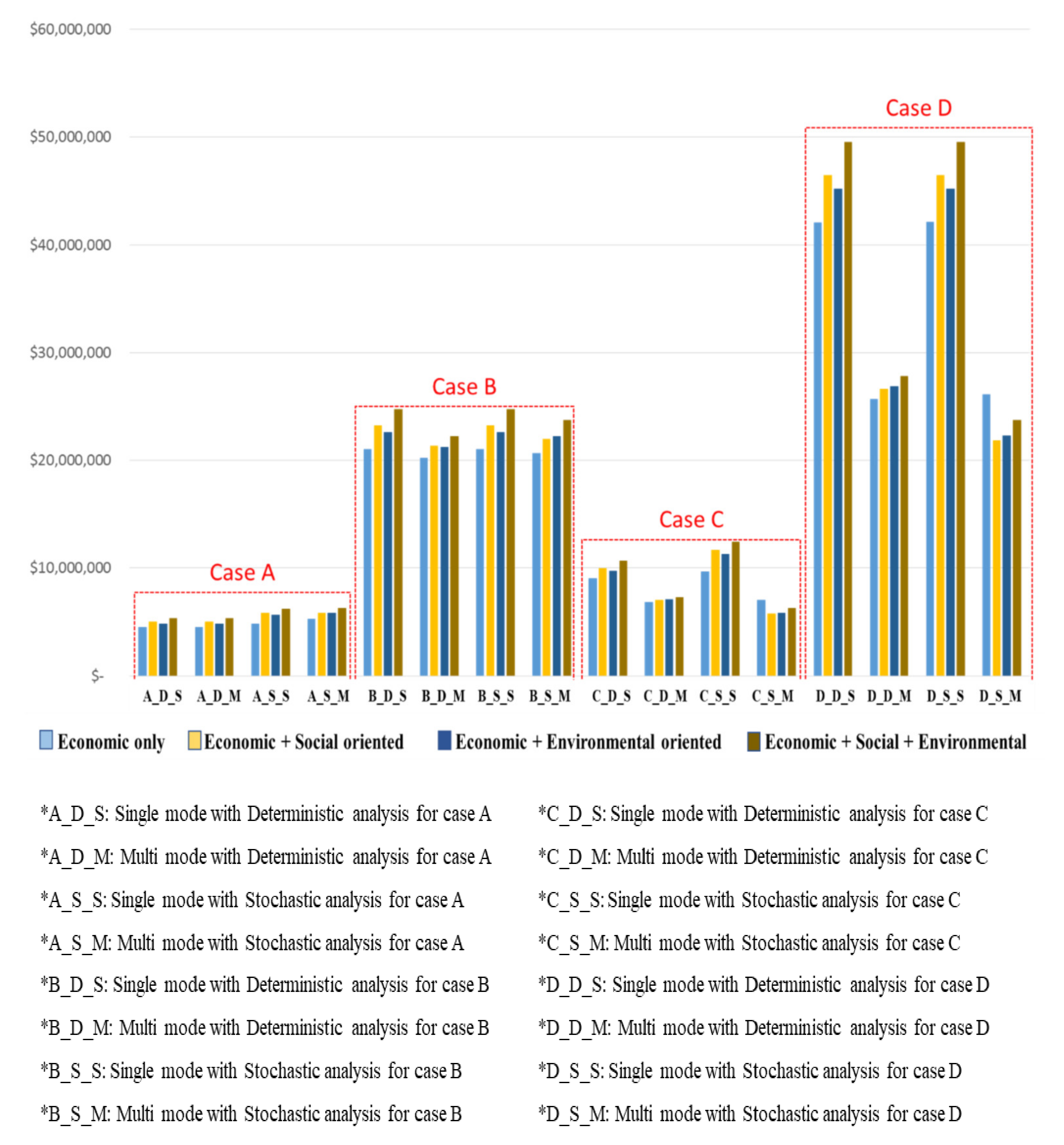
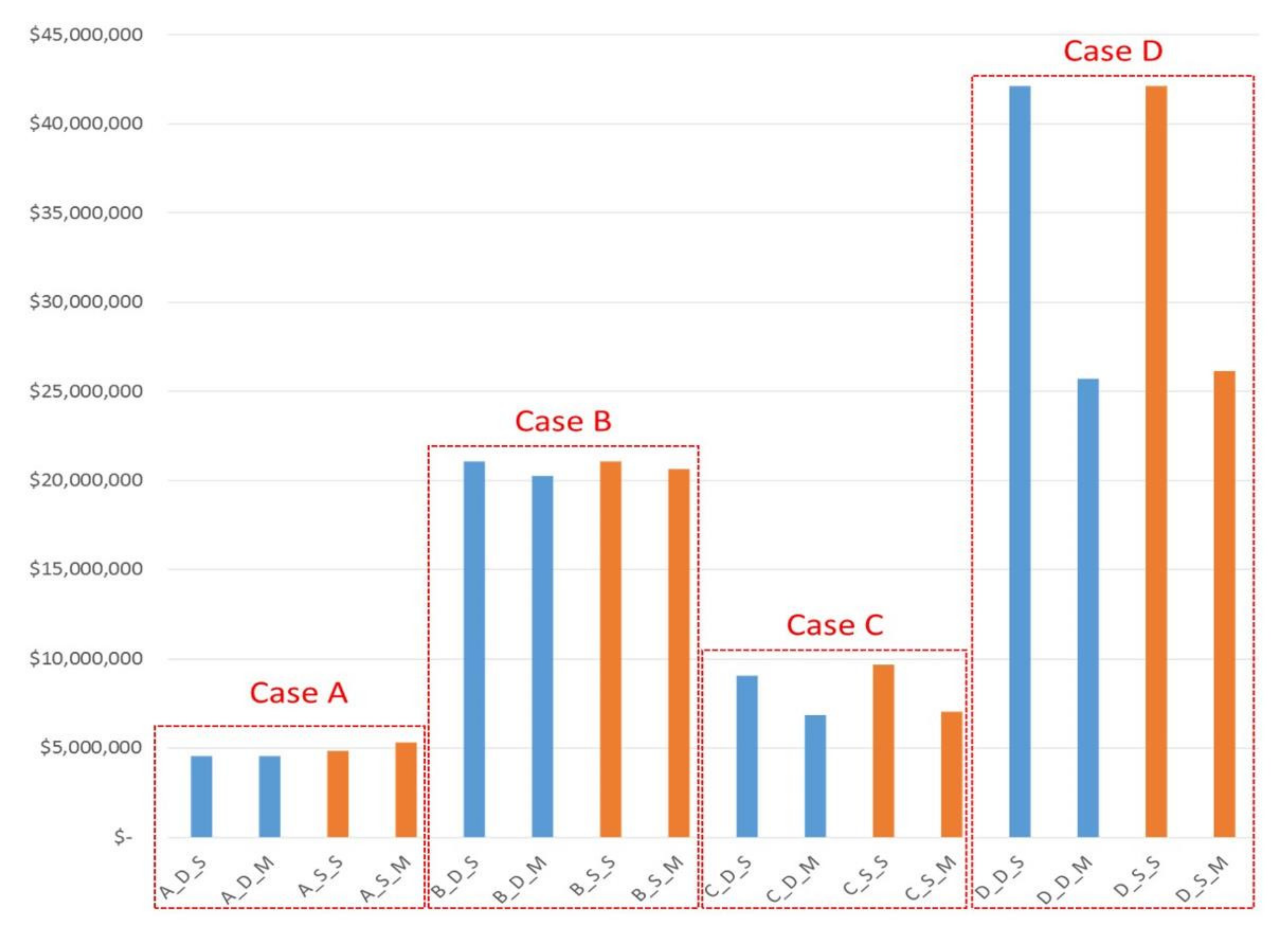
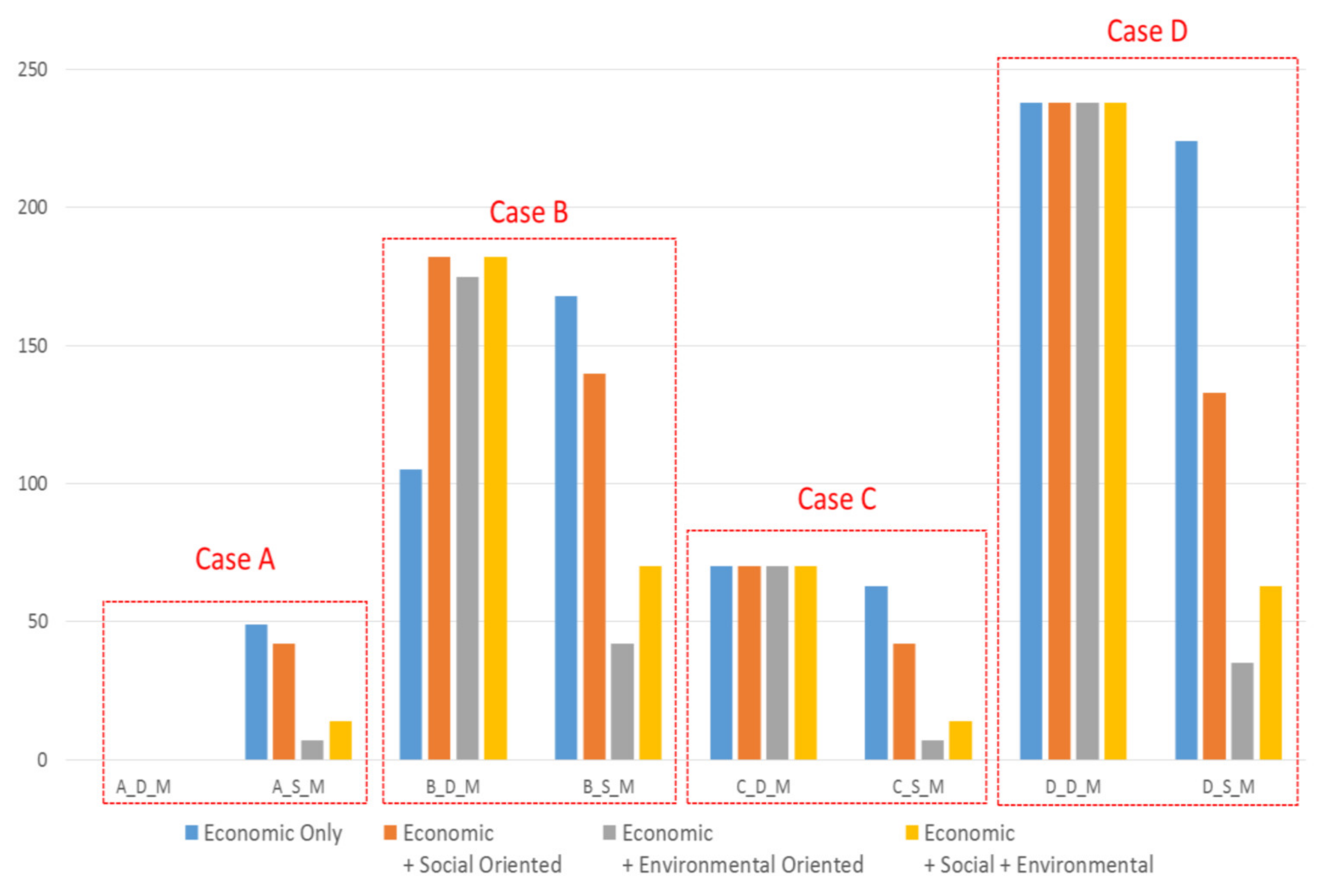
2.3. Numerical Example: 4 Cases

As shown in Figure 1, a total of 187 bio-electricity plants currently use woody biomass in a form of woods solids (WDS) as a plant primary fuel in the US. In terms of plant nameplate capacity, the annual capacity of 75% of the 187 plants is less than 47 MW [21]. As seen in Figure 1, most of the bio-electricity plants using wood solids do not currently need high quantities of woody feedstock. The average capacity of all these plants is 37 MW. Considering a typical case of biomass plants, less than 500,000 tons of woody feedstocks are procured from collecting areas to produce about 50 MW capacity annually.

In this study, 60% and 99% percent of a plant’s capacity were considered as target example cases. Plants at these percentile capacities normally need about 350,000 and 1,200,000 tons of annual woody biomass, respectively.

Meanwhile, the average procurement distance for biomass feedstock is also a critical criterion to classify bio-electricity plants. The breakpoints of economic distance for each mode of transportation are presented variously in previous studies as shown in

Table 2. The Economic Distances by Modes for Biomass Transportation.

Feedstock	Truck	Rail	Ship	Region	Reference
Forest	~100 km<	<100 km~		Natherland	[22]
Forest	~50 km<	<50~200 km<	<200~1200 km<	Spain	[23]
Woodchip	~145 km<	<145 km~		Canada (Unit Train)	[24]
Woodchip	~386 km<	<386 km~		US (Unit Train)	[25]
Woodchip	~500 km<	<500 km~	<800 km~	Canada (Unit Train)	[26]
straw	~170 km<	<170 km~		Canada (Unit Train)	[24]
straw	~500 km<	<500 km~	<1500 km~	Canada (Unit Train)	[26]
corn stover	~500 km<	<500 km~	<1500 km~	US (Unit Train)	[26]
corn stover	~170 km<	<170 km~		Canada (Unit Train)	[24]
Grain	~161 km<	<161 km~		US (Unit Train)	[25]
Grain	~338 km<	<338 km~		US (Unit Train)	[25]

.

In this study, we selected 75 miles (120 km) and 150 miles (240 km) as average distance criteria for procurement, considering a marginal economic distance of the trucking system for forest and woody biomass. A numerical analysis is then possible for a total of four different cases using two conditions for classification: annual capacity of feedstock and average procurement distance, as follows:

• Case A: Low annual capacity and Short procurement distance for feedstock;
• Case B: High annual capacity and Short procurement distance for feedstock;
• Case C: Low annual capacity and Long procurement distance for feedstock;
• Case D: High annual capacity and Long procurement distance for feedstock.

Table 3. Numerical example cases of bio-electricity plants for this study.

Annual Capacity	350,000 Tons	1,200,000 Tons
Avg. Distance
75 miles	Case: A	Case: B
150 miles	Case: C	Case: D

indicates these example cases of four strategies for bio-electricity plants in this study.

The next step is to relate the identification of input sources to their values used in this sustainable biomass transportation model. Since most of the data under basic conditions are case-specific, such as the kind of mode type that is possible to use and the number of conversion plants or collecting areas, operational data need to be assumed based on the four different cases above. The values of three sustainable factors are mainly utilized from previous research which suggested some pertinent rules of thumb and empirical data with regards to biomass transportation.

Table 4. Example values of input parameters for stochastic optimization model.

Input Category		Values of Each Case
		Case A	Case B	Case C	Case D
Conditions	Possible Mode types	Truck	Truck,	Truck,	Truck,
		Rail	Rail	Rail	Rail
	Number of collecting areas	3	3	3	3
	Annual capacity of each collecting areas (Tons)	N~(300,000, 10,000)	N~(300,000, 10,000)	N~(300,000, 10,000)	N~(300,000, 10,000)
		N~(400,000, 50,000)	N~(400,000, 50,000)	N~(400,000, 50,000)	N~(400,000, 50,000)
		N~(500,000, 200,000)	N~(500,000, 200,000)	N~(500,000, 200,000)	N~(500,000, 200,000)
	Number of	1	1	1	1
	conversion plants
	Distance (Mile) from collecting area and plant	Avg. 75	Avg. 75	Avg. 150	Avg. 150
	Distance (Mile) from collecting area rail siding	Avg. 20	Avg. 20	Avg. 40	Avg. 40
	Distance (Mile) from rail siding and plant	Avg. 60	Avg. 60	Avg. 120	Avg. 120
Economic cost	Demand quantities	N~(350,000, 1000)	N~(1,200,000, 5000)	N~(350,000, 1000)	N~(1,200,000, 5000)
	(Tons)
	Supply quantities	N~(350,000, 1000)	N~(1,200,000, 5000)	N~(350,000, 1000)	N~(1,200,000, 5000)
	(Tons)
	Unit costs per tonnage for hauling	Truck: N~(0.14, 0.01)	Truck: N~(0.14, 0.01)	Truck: N~(0.14, 0.01)	Truck: N~(0.14, 0.01)
factors	(US $/Dry ton/km, [17])	Rail:	Rail:	Rail:	Rail:
		N~(0.03, 0.001)	N~(0.03, 0.001)	N~(0.03, 0.001)	N~(0.03, 0.001)
	Unit costs of loading/unloading for rail	N~(4.8, 0.4)	N~(4.8, 0.4)	N~(4.8, 0.4)	N~(4.8, 0.4)
	(US $/Dry ton, [16])
	unit costs of	N~(400, 100)	N~(400, 100)	N~(400, 100)	N~(400, 100)
	leasing a railcar
	(US $/month, [18])
Social cost	Traffic Congestion	Truck: N~(0.66, 0.2)	Truck: N~(0.66, 0.2)	Truck: N~(0.66, 0.2)	Truck: N~(0.66, 0.2)
		Rail:	Rail:	Rail:	Rail:
	(US cent/ton-mile, [19])	N~(0.015, 0.1)	N~(0.015, 0.1)	N~(0.015, 0.1)	N~(0.015, 0.1)
factors	Accident Risk	Truck: N~(1.66, 2)	Truck: N~(1.66, 2)	Truck: N~(1.66, 2)	Truck: N~(1.66, 2)
		Rail:	Rail:	Rail:	Rail:
	(US cent/ton-mile, [19])	N~(0.018, 0.5)	N~(0.018, 0.5)	N~(0.018, 0.5)	N~(0.018, 0.5)
Environmental cost	Costs of Emissions	Truck: N~(0.71, 0.5)	Truck: N~(0.71, 0.5)	Truck: N~(0.71, 0.5)	Truck: N~(0.71, 0.5)
	: PM and NOx	Rail:	Rail:	Rail:	Rail:
	(US cent/ton-mile, [16])	N~(0.19, 2)	N~(0.19, 2)	N~(0.19, 2)	N~(0.19, 2)
factors	Costs of Emissions	Truck: N~(0.22, 0.5)	Truck: N~(0.22, 0.5)	Truck: N~(0.22, 0.5)	Truck: N~(0.22, 0.5)
	: CO2	Rail:	Rail:	Rail:	Rail:
	(US cent/ton-mile, [16])	N~(0.05, 1)	N~(0.05, 1)	N~(0.05, 1)	N~(0.05, 1)

presents the list of input data for four example cases with uncertainty. Note that it is assumed there are three areas to collect biomass feedstocks. In all cases, it is also assumed that a quantity of each market demand is covered with their processing quantities from each collecting area. All uncertain parameters $\xi =(C_X, C_Y, C_Z, C_K, R_X, R_Y,R_Z,E_X, E_Y, E_Z, Q, O, a)$ are regarded as independent of each other, as well as normally distributed

Note that available estimates used different methods and assumptions for determining the average of each factor, and variations are also assumed by the authors. Unit costs per tonnage for hauling and transloading are based on previous studies [16,17,18]. For social cost factors, we selected traffic congestion and accident risk from the research of the US Governmental Accountability Office (GAO) [19]. The environmental cost factors are based on air emissions (GHG, PM, and NOx) from feedstock transportation by truck and rail [16].

If the decision maker is interested in a satisfying solution with α = 0.99 and β = 0.99 for all cases, then it is possible to solve the following problem by using the stochastic optimization model (11). For example, Case A would be transformed to non-linear integer program as follows:

MIN

((w₁ × 55 × 28 × 0.224) + (w₂ × 55 × 28 × (0.0066 + 0.0166)) + (w₃ × 55 × 28 × (0.0071 + 0.0071 + 0.0022))) × X₁ +

((w₁ × 75 × 28 × 0.224) + (w₂ × 75 × 28 × (0.0066 + 0.0166)) + (w₃ × 75 × 28 × (0.0071 + 0.0071 + 0.0022))) × X₂ +

((w₁ × 95 × 28 × 0.224) + (w₂ × 95 × 28 × (0.0066 + 0.0166)) + (w₃ × 95 × 28 × (0.0071 + 0.0071 + 0.0022))) × X₃ +

(w₁ × ((10 × 28 × 0.224) + (28 × 4.8)) + w₂ × (10 × 28 × (0.0066 + 0.0166)) + w₃ × ((10 × 28 × (0.0071 + 0.0071 + 0.0022)))) × Y₁ +

(w₁ × ((20 × 28 × 0.224) + (28 × 4.8)) + w₂ × (20 × 28 × (0.0066 + 0.0166)) + w₃ × ((20 × 28 × (0.0071 + 0.0071 + 0.0022)))) × Y₂ +

(w₁ × ((30 × 28 × 0.224) + (28 × 4.8)) + w₂ × (30 × 28 × (0.0066 + 0.0166)) + w₃ × ((30 × 28 × (0.0071 + 0.0071 + 0.0022)))) × Y₃ +

(w₁ × ((60 × 5000 × 0.048) + (5000 × 4.8)) + w₂ × (60 × 5000 × (0.00015 + 0.00018)) + w₃ × ((60 × 5000 × (0.0019 + 0.0019 + 0.0005)))) × Z +

(w₁ × 4800 × K) +

2.33 × (((w₁^2 × 55^2 × 28^2 × 0.01) + (w₂^2 × 55^2 × 28^2 × (0.2 + 2)) + (w₃^2 × 55^2 × 28^2 × (0.5 + 0.5 + 0.5))) × X₁^2 +

((w₁^2 × 75^2 × 28^2 × 0.01) + (w₂^2 × 75^2 × 28^2 × (0.2 + 2)) + (w₃^2 × 75^2 × 28^2 × (0.5 + 0.5 + 0.5))) × X₂^2 +

((w₁^2 × 95^2 × 28^2 × 0.01) + (w₂^2 × 95^2 × 28^2 × (0.2 + 2)) + (w₃^2 × 95^2 × 28^2 × (0.5 + 0.5 + 0.5))) × X₃^2 +

(w₁^2 × ((10^2 × 28^2 × 0.01) + (28^2 × 0.4)) + (w₂^2 × 10^2 × 28^2 × (0.2 + 2)) + (w₃^2 × 10^2 × 28^2 × (0.5 + 0.5 + 0.5))) × Y₁^2 +

(w₁^2 × ((20^2 × 28^2 × 0.01) + (28^2 × 0.4)) + (w₂^2 × 20^2 × 28^2 × (0.2 + 2)) + (w₃^2 × 20^2 × 28^2 × (0.5 + 0.5 + 0.5))) × Y₂^2 +

(w₁^2 × ((30^2 × 28^2 × 0.01) + (28^2 × 0.4)) + (w₂^2 × 30^2 × 28^2 × (0.2 + 2)) + (w₃^2 × 30^2 × 28^2 × (0.5 + 0.5 + 0.5))) × Y₃^2 +

((w₁^2 × (60^2 × 5000^2 × 0.001) + (5000^2 × 0.4)) + (w₂^2 × 60^2 × 5000^2 × (0.1 + 0.5)) + (w₃^2 × 60^2 × 5000^2 × (2 + 2 + 1))) × Z^2 +

100 × K^2)^0.5;

S.T.

[R1] (28 × X₁) + (28 × Y₁) − 300,000 + (2.33 × 10,000^0.5) <= 0;

[R2] (28 × X₂) + (28 × Y₂) − 400,000 + (2.33 × 50,000^0.5) <= 0;

[R3] (28 × X₃) + (28 × Y₃) − 700,000 + (2.33 × 200,000^0.5) <= 0;

[R4] (28 × X₁) + (28 × X₂) + (28 × X₃) + (5000 × Z) − 350,000 + (2.33 × 1000^0.5) >= 0;

[R5] (28 × Y₁) + (28 × Y₂) + (28 × Y₃) = (5000 × Z;

[R6] Z <= K × 10,000,000;

$$V=\left\{X_i, Y_i, Z, K\right\}=Positive Integer \forall i\in I, K \in \left\{0, 1\right\}$$

3. Results and Discussions

The mathematical model was applied to the four numerical examples described in Table 4. In all cases, the analysis was conducted with four combinations in terms of orientation of sustainable factors: (1) economic only, (2) economic and social oriented, (3) economic and environmental oriented, and (4) economic, social, and environmental oriented. Each combination can be controlled by weighting factors $w_1$ (Economic), $w_2$ (Social), and $w_3$ (Environmental). When external costs (social cost and environmental cost) are fully considered, weighting factors $w_1$ = $w_2$ = $w_3$ = 1. If we calculate the transportation cost excluding the external costs, weighting factor $w_1$ = 1 and $w_2$ = $w_3$ = 0. Figure 2 presents the results of the optimization problem for four cases which are combined with deterministic and stochastic analyses. For all cases, we compared the cost difference between single mode (truck only) and multimodal (truck and rail) biomass transportation.

This figure also suggests the different results of optimized annual number of truck and rail hauling, as well as minimized transportation costs regarding four different cases in perspective of annual capacity and procurement distance options.

According to this result, the optimized cost of biomass transportation considering the economic factor only is generally less than when under consideration of other sustainable factors. The trend of increasing costs, however, is various for each case. Particularly for the case of multi modal with stochastic analysis for Case D (D_S_M in Figure 2), the optimized cost is highest when we only consider economic factors. This may be related to the findings of Ko et al. (2016) that external costs of transportation are strongly associated with distance and tonnage [16]. In other words, shipments using rail can significantly decrease the external costs in cases where high volume is transported for long distance between origins and destinations.

Figure 3 describes the cost savings between single and multimodal transportation for each case. Along with increased distance and volume, cost savings from utilizing multimodal transportation increase for all scenarios. The results indicate that inclusion of external transportation costs and growth of plant capacity both escalate the share of rail shipments while trying to minimize total transportation costs.

We found that more cost savings from multimodal transportation can be identified if we analyze transportation costs with stochastic modeling. This effect is more remarkable when the bioenergy plant is located far from the biomass collecting site (Case C and D). In the case of short-distance cases (Case A and B), it reveals that the impact of utilization of stochastic methods is insignificant, as the costs savings from multimodal transportation is trivial.

In general, most industries are interested in optimization costs in the economic perspective only. Figure 4 shows the optimized transportation costs when we regard economic parameters as the only sustainable factor. Note that experimental results from the deterministic approach (blue color) is distinguished with the results from the stochastic model (orange color) by their colors. In most cases, it shows that multimodal transportation could provide cost savings in the economic cost factor, except in the case of A (low annual capacity and short procurement distance for feedstock). In particular, if we analyze this problem with uncertainty, the cost increases instead (in A_S_M). We surmise that this result may arise since the economic benefit of multimodal transportation cannot cover the variance of increased parameters. When it comes to the effect of the stochastic method, there is also no great difference in optimized costs with deterministic analysis in all cases. Strange as it may seem, it is understandable because these cost gaps are covered with other combinations of transportation modes. In other words, selecting the stochastic method has more significant effects on the modal share than on the whole economic costs savings.

Figure 5, which shows the annual number of rail shipping for each multimodal case, can support this assumption. It can be seen that rail transportation can be used in various cases as a multimodal option for the achievement of optimized costs. This means the modal share between truck and rail varies for each case. The result of Case A reveals an interesting point: that the need for rail shipment arises when the analysis is conducted by stochastic approach, while other cases show reversed patterns. If we compare the results between Figure 3 and Figure 5, we can see the number of rail shipments in Case B is much higher than Case C, though the cost savings of Case B are lower than Case C. This means that the increase of rail shipments does not lead to an increase in cost savings. Thus, it can be concluded that the distance between plant and biomass collecting sites is a more significant factor which affects the benefit of multimodal transportation with rail compared to the capacity of bioenergy plants. Figure 5 also indicates that there would be very little chance of rail shipments for Case A_D_M. This is evident from a previous study [16] that found that direct truck haulage dominates shipment scenarios that cover short distances with small-capacities, as delivery by rail is selected only for large-capacity scenarios.

4. Conclusions

This study investigates transportation costs when using biomass feedstock for electricity plants. More specifically, it attempts to identify and minimize transportation costs, using either single or multimodal transportation. The analysis was conducted through deterministic and stochastic mathematical models that minimize transportation costs, including economic and/or external costs.

The models were tested with four cases classified in terms of a bioenergy plant’s annual capacity and the average distance between biomass collecting sites and the plant. The experimental results show that while the optimized costs of biomass transportation that consider only economic factors is generally less than when under consideration for other sustainable factors, the trend of increasing costs are various for each case. It is also found that more cost savings from multimodal transportation can be identified if we analyze transportation costs with stochastic modeling. This effect is more remarkable when the bioenergy plant is located far from the biomass collecting site. In the case of short-distance plant cases, this reveals that the impact of utilization of stochastic methods is insignificant, as the cost savings from multimodal transportation is trivial. Other findings from our experiments include how multimodal transportation may provide cost savings in the economic cost factor, except in the case of low annual capacity and short average distance. When it comes to the effect of the stochastic method, there is also no great difference in optimized costs with deterministic analysis in all cases. This is understandable because we found that selecting the stochastic method more significantly effects the modal share than the entire economic cost savings. Finally, the experimental results reveal the modal share between truck and rail varies for each case, as rail transportation can be used in various cases as a multimodal option to achieve optimized costs. One of the interesting points is that increase of rail shipments does not necessarily lead to the increase of cost savings. This tells us that the distance between the plant and biomass collecting site is a more significant factor which affects the benefit of multimodal transportation with rail compared to the capacity of the bioenergy plant.

The main contributions of this study include the development of a simple approach to the multi-objective stochastic model for sustainable biomass transportation systems. We also identified the impact level of model selection (deterministic and stochastic) on transportation mode (single and multimodal transportation). Though this study tried to use as much actual experimental data as possible, it is recognized that several assumptions were made, such as the truck and rail operations. In addition, there were certain limitations that should be noted when interpreting the results. For example, exclusion of feedstock seasonality, and the loading/unloading process. In future studies, access to more actual cost data would facilitate the development of more accurate tools to figure out the role of the stochastic method, as well as the benefits of multimodal transportation for bioenergy production.

References

1. Cundiff, J.S.; Dias, N.; Sherali, H.D. A linear programming approach for designing a herbaceous biomass delivery system. Bioresour. Technol. 1997, 59, 47–55. [Google Scholar] [CrossRef]
2. Zhu, X.Y.; Li, X.; Yao, Q.; Chen, Y. Challenges and models in supporting logistics system design for dedicated-biomass-based bioenergy industry. Bioresour. Technol. 2011, 102, 1344–1351. [Google Scholar] [CrossRef] [PubMed]
3. Devlin, G.; Talbot, B. Deriving cooperative biomass resource transport supply strategies in meeting co-firing energy regulations: A case for peat and wood fibre in Ireland. Appl. Energy 2014, 113, 1700–1709. [Google Scholar] [CrossRef] [Green Version]
4. Sosa, A.; Acuna, M.; McDonnell, K.; Devlin, G. Managing the moisture content of wood biomass for the optimisation of Ireland’s transport supply strategy to bioenergy markets and competing industries. Energy 2015, 86, 354–368. [Google Scholar] [CrossRef]
5. Osmani, A.; Zhang, J. Optimal grid design and logistic planning for wind and biomass based renewable electricity supply chains under uncertainties. Energy 2014, 70, 514–528. [Google Scholar] [CrossRef]
6. Cucek, L.; Martin, M.; Grossmann, I.E.; Kravanja, Z. Multi-period synthesis of optimally integrated biomass and bioenergy supply network. Comput. Chem. Eng. 2014, 66, 57–70. [Google Scholar] [CrossRef]
7. Poudel, S.R.; Marufuzzaman, M.; Bian, L. A hybrid decomposition algorithm for designing a multi-modal transportation network under biomass supply uncertainty. Transp. Res. Part E Logist. Transp. Rev. 2016, 94, 1–25. [Google Scholar] [CrossRef]
8. Dal Mas, M.; Giarola, S.; Zamboni, A.; Bezzo, F. Capacity planning and financial optimization of the bioethanol supply chain under price uncertainty. Comput. Aided Chem. Eng. 2010, 28, 97–102. [Google Scholar]
9. You, F.; Grossmann, I.E. Design of responsive supply chains under demand uncertainty. Comput. Chem. Eng. 2008, 32, 3090–3111. [Google Scholar] [CrossRef]
10. Kim, J.; Realff, M.J.; Lee, J.H.; Whittaker, C.; Furtner, L. Design of biomass processing network for biofuel production using an MILP model. Biomass Bioenergy 2011, 35, 853–871. [Google Scholar] [CrossRef]
11. Ravula, P.P.; Grisso, R.D.; Cundiff, J.S. Comparison between two policy strategies for scheduling trucks in a biomass logistic system. Bioresour. Technol. 2008, 99, 5710–5721. [Google Scholar] [CrossRef] [PubMed]
12. Simwanda, M.; Wing, M.G.; Sessions, J. Evaluating global positioning system accuracy for forest biomass transportation tracking within varying forest canopy. West. J. Appl. For. 2011, 26, 165–173. [Google Scholar] [CrossRef] [Green Version]
13. Han, S.K.; Murphy, G.E. Solving a woody biomass truck scheduling problem for a transport company in Western Oregon, USA. Biomass Bioenergy 2012, 44, 47–55. [Google Scholar] [CrossRef]
14. Jones, G.; Loeffler, D.; Butler, E.; Hummel, S.; Chung, W. The financial feasibility of delivering forest treatment residues to bioenergy facilities over a range of diesel fuel and delivered biomass prices. Biomass Bioenergy 2013, 48, 171–180. [Google Scholar] [CrossRef]
15. Abbas, D.; Arnosti, D. Economics and Logistics of Biomass Utilization in the Superior National Forest. J. Sustain. For. 2013, 32, 41–57. [Google Scholar] [CrossRef]
16. Ko, S.; Lautala, P.; Fan, J.; Shonnard, D.R. Economic, social, and environmental cost optimization of biomass transportation: A regional model for transportation analysis in plant location process. Biofuel Bioprod. Biorefin. 2019, 13, 582–598. [Google Scholar] [CrossRef]
17. Kumar, A.; Sokhansanj, S.; Flynn, P.C. Development of a multicriteria assessment model for ranking biomass feedstock collection and transportation systems. Appl. Biochem. Biotechnol. 2006, 129, 71–87. [Google Scholar] [CrossRef]
18. Tita, B. Railcar Shortage in US Pushes Up Lease Rates. The Wall Street Journal. 2014. Available online: https://www.wsj.com/articles/railcar-shortage-in-u-s-pushes-up-lease-rates-1401393331 (accessed on 1 September 2020).
19. GAO. Transportation Surface Freight: A comparison of the Costs of Road, Rail, and Waterways Freight Shipments That Are Not Passed on to Consumers. 2011, GAO-11-134. Available online: https://www.gao.gov/assets/gao-11-134.pdf (accessed on 15 November 2020).
20. Kampempe, J.D.B.; Luhandjula, M.K. Chance-constrained approaches for multiobjective stochastic linear programming problems. Am. J. Oper. Res. 2012, 2, 519–526. [Google Scholar] [CrossRef] [Green Version]
21. US EIA. Form EIA-860 Detailed Data with Previous form Data: Year 2020. 2021, Washington, DC. Available online: https://www.eia.gov/electricity/data/eia860/ (accessed on 1 September 2021).
22. Hamelinck, C.N.; Suurs, R.A.A.; Faaij, A.P.C. International bioenergy transport costs and energy balance. Biomass Bioenergy 2005, 29, 114–134. [Google Scholar] [CrossRef]
23. Ruiz, J.A.; Juarez, M.C.; Morales, M.P.; Munoz, P.; Mendivil, M.A. Biomass logistics: Financial & environmental costs. Case study: 2 MW electrical power plants. Biomass Bioenergy 2013, 56, 260–267. [Google Scholar]
24. Mahmudi, H.; Flynn, P.C. Rail vs truck transport of biomass. Appl. Biochem. Biotechnol. 2006, 129, 88–103. [Google Scholar] [CrossRef]
25. Gonzales, D.; Searcy, E.M.; Eksioglu, S.D. Cost analysis for high-volume and long-haul transportation of densified biomass feedstock. Transp. Res. 2013, 49, 48–61. [Google Scholar] [CrossRef]
26. Searcy, E.; Flynn, P.; Ghafoori, E.; Kumar, A. The relative cost of biomass energy transport. Appl. Biochem. Biotechnol. 2007, 137, 639–652. [Google Scholar] [PubMed]
Figure 1. The name plate capacity (MW) of bio-electricity plants in US [21].
Sustainability 14 01889 g001
Figure 2. Results of Optimized transportation costs for each case.
Sustainability 14 01889 g002
Figure 3. Cost Savings between Single and Multimodal Transportation.
Sustainability 14 01889 g003
Figure 4. Optimized transportation costs considering economic factor only.
Sustainability 14 01889 g004
Figure 5. Annual number of rail shipments for each multimodal case.
Sustainability 14 01889 g005