Analytical Modeling of Solute Transport in a Two-Zoned Porous Medium Flow

Abstract

The objective of this study is to model the transport of groundwater contamination in one-layered and two-zoned porous medium flows by an analytical approach. The one-dimensional advection–dispersion equation (ADE) has usually been used to describe the problems of pollutant transport in a water environment. This study presents some exact solutions to the one-dimensional ADE to examine the variation of solute concentration with and without the biodegradable effect in an unconfined aquifer of a finite domain by the generalized integral transform method (GITM). The modeling results for the concentration of groundwater contamination show that the pollutant concentration is more sensitive to the Peclect number than to the retardation factor and the first-order decaying coefficient in uniform groundwater flow. In composite soil zones, decaying and diffusion factors have significant effects on the contamination concentration around the interface, especially over a long-term period. The transport flux between the two regions is determined by the concentration gradient at the interface of the two regions. The contaminated concentration decreases as the retardation factor, Peclect number, and the first-order decaying coefficient increase for every location at a fixed duration. Moreover, the contaminated concentration is more sensitive to the Peclect number than to the retardation factor and the first-order decaying coefficient in uniform groundwater flow.

1. Introduction

Groundwater is overconsumed in some regions or countries where people regard it as a crucial water resources. Therefore, if groundwater is contaminated by artificial activities such as pesticide usage, waste products from construction or industrial factory, and excrements of livestock, it may threaten human health after people drink it over the long term. Once groundwater is contaminated, it is difficult to purify it and requires huge treatment costs.

Schuetz et al. [1] constructed an experimental wetland to realize the migration of solutes in shallow water using a novel solute tracking method. The test was to inject hot water into the model and observe the water flow with a handheld thermal imaging system. This model can easily confirm the solute movement in shallow water flow and can simulate more complex topographic structures according to the local topographic variation model. Rubol et al. [2] used the advection–dispersion equation (ADE) with spatially variable coefficients to model solute transport in soil layers with plant roots. The semi-analytical solution of solute transport in the submerged vegetation aquatic system is derived by the integral transformation technique. Irregularity of the soil layer with plant roots affects the soil infiltration rate, which further affects the symmetry of concentration, effective vertical diffusion, and magnitude of peak concentration. These flow mechanisms depend on the geometry of the soil layer with the plant roots and affect the concentration of solutes in the water flow, which are critical for studies on improving groundwater quality.

The unidimensional advection–dispersion equation (ADE) is the most commonly used partial differential equation that delineates the solute transport distribution in time and space. Such an equation is derived with respect to the hydro-dynamic dispersion process in aquifers according to the law of conservation of mass. Analytical solutions to ADE with constant coefficients have been obtained, subject to a distinct set of initial and boundary conditions in recent decades. Fry et al. [3] derived an analytical solution to the solute transport equation by an eigenfunction integral equations method to discuss the variation of concentrations under the effect of rate-limited desorption and decay. In the process of derivation, a partial solution is first obtained by temporarily removing one term in the original equation, and then the full solution can be found by adding the additional term to the partial solution in order to satisfy the original full equation. The solution’s procedure is complicated.

Among the existent methods used to solve ADE, Laplace transform technique is the most popular method. Therefore, some articles using Laplace transform methods are surveyed here. Kumar et al. [4] presented an analytical solution of one-dimensional ADE with variable coefficients in a finite domain for two dispersion problems by employing the Laplace transform method. Their so-called variable coefficients—solute dispersion and average flow velocity—are constrained to a specific mathematical relation. Later, Kumar et al. [5] used the Laplace transform technique again to deal with similar problems in the semi-infinite media. Neelz [6] commented that the limitations of an analytical solution for ADE with spatially variable coefficients should be noted. Jaiswal et al. [7] applied the Laplace transform method to solve the linearized advection–diffusion equation and obtained analytical solutions for temporally and spatially dependent solute concentrations for a source of the pulse input type along a uniform/non-uniform flow in a semi-infinite length. The pulse type input concentration was imposed by a constant and a variable way, respectively. Moreover, Jaiswal et al. [8] also employed the Laplace transform technique to deal with a similar problem with a source input concentration for uniform dispersion in a uniform flow where the dispersion parameter is not proportional to the flow velocity.

Heterogeneous soil layers are widely present in subsurface environments, as delineated by Liang et al. [9], in which solute transport in heterogeneous media was simulated by a one-dimensional two-domain model, and the results were verified by comparing the numerical and analytical solutions. From their results, the exchange of solute concentrations between the two regions was caused by the difference of properties of the two regions and is determined by the lateral dispersion at the interface. As solutes pass through these two layers, part of the solute in the fast-flow region migrates to the slow-flow region first, and then this concentration exchange reverses; that is, part of the solute in the slow-flow region migrates back to the fast-flow region. The interaction of the solute has a significant effect on pollution in groundwater systems.

Perez Guerrero and Skaggs [10] and Perez Guerrero et al. [11] described the transport of pollutants in heterogeneous porous media as usually formulated by an advection–diffusion equation, and thus, an analytical solution was proposed. This system, composed of differential equations, has constant coefficients for both transient and steady-state problems. After comparing it with the previous hybrid analytical–digital solution obtained by directly applying GITM, the new presented solution converges faster.

In a one-dimensional convection–diffusion equation with time-varying coefficients, the solute diffusion parameter and the solute flow are various with time. Such a problem was analytically solved by Jaiswal et al. [7] by Laplace transform technique, and in their study, the dispersion of a continuous input point source in the initially solute-free semi-infinite domain was studied.

Kumar et al. [12] solved the one-dimensional convection–diffusion equation with three various solute dispersion coefficients. In the semi-infinite medium, continuous point sources with uniform and increasing properties were considered. They also used the Laplace transform technique to obtain analytical solutions. The spreading was considered to be related to the square of the space-related velocity, and new independent variables were introduced through separate transformations. According to these transformations, the convection–diffusion equation in each problem was simplified to an equation with constant coefficients.

Conversely, Schmid [13] also derived solutions considering the first-order decay advection–dispersion effect in rivers with transient storage zones by the Laplace transform method. The results were compared with numerical solutions by a finite difference method, and they obtained fairly good agreement. Additionally, Shukla [14] presented analytical solutions to 1D ADE, including the effect of the first-order decay rate of the pollutant BOD by the Fourier transform method for the case of unsteady transport dispersion of non-conservative pollutants in a river. Shukla [14] found that an increase in the pollutant decay rate, as well as convective velocity and dispersion, increases memory length and decreases memory time.

In the past, there were few studies on analytical approaches for solute transport in double-layer systems. Gureghian and Jansen [15] developed a one-dimensional analytical solution for the radionuclide decay chain in a semi-infinite double-layer medium. Ledger et al. [16] proposed an analytical solution for one-dimensional transport in double-layer media with the help of Laplace transform. The model they established included the continuity of concentration at the interface and the conservation of mass flux. Since the solution of double-layer porous media in the Laplace domain became extremely complicated, the numerical Laplace inverse transform time domain solution was used. Leij and van Genuchten [17] derived a semi-analytical solution with a clear mathematical expression in the time domain of solute transport in double-layer porous media. Li and Cleall [18] proposed a one-dimensional analytical solution for solute transport in a two-layer medium, considering five different combinations of inflow and outflow boundary conditions. Perez Guerrero et al. [19] applied the classic integral transformation technique to develop a closed-form analytical solution for transmission in multi-layer media. Recently, Batu [20] proposed an analytical solution for solute transport in semi-infinite, dual-domain media, considering biodegradation. Chen et al. [21] proposed a one-dimensional stable design equation for the PRB system. This design equation is obtained based on the work of van Genuchten [22], presenting a one-dimensional analytical solution for a steady-state groundwater flow in a proposed infinite single-domain medium. Chen et al. [23] described the minimum thickness of PRB by developing a single-domain analytical solution with zero concentration gradient on the exit boundary of PRB. Park and Zhan [24] and Chen et al. [25] respectively proposed one-dimensional and two-domain analytical solutions for single and multiple species transport in a PRB system. Based on the forgoing statements, most of the above studies are still limited to one-zoned problems in one-dimensional transportation systems, and most researchers employed the Laplace transform technique to solve the solute transport equation with and without considering the effect of the first-order decay rate. In this study, a generalized integral transform technique was applied instead for a two-zoned problem because of its steady and fast convergence as discussed in the work of Wu and Hsieh [26].

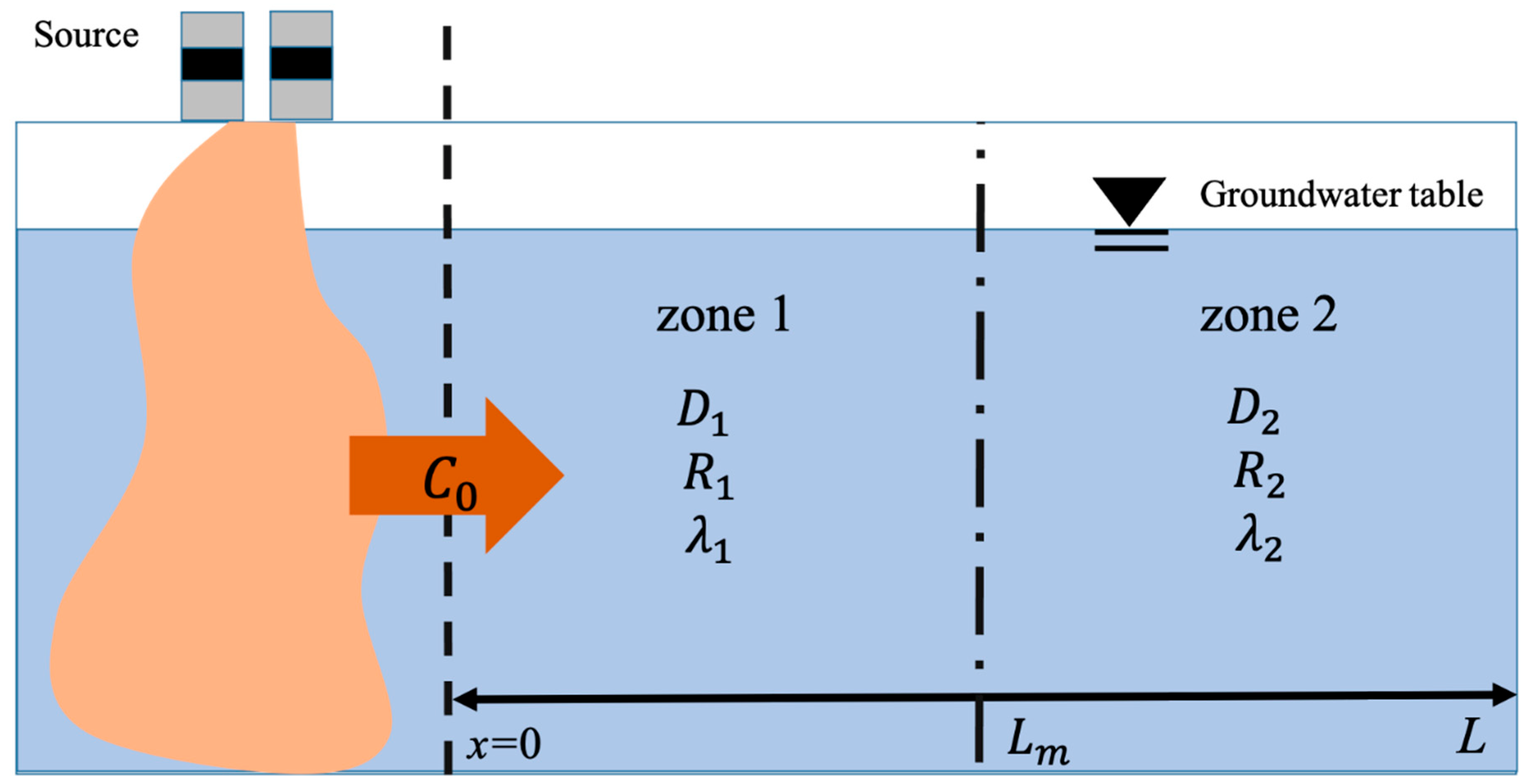
The purpose of this study was to analyze the transport of groundwater contamination in one- and two-zoned porous medium flows via an analytical mathematical model. This study provides some precise solutions for one-dimensional ADEs to examine changes in solute concentrations in unconfined aquifers with or without biodegradable effects by GITM. The solutions obtained by GITM converge fast, and the current solutions have been verified with numerical solutions. The modeling results of groundwater pollution concentration show that the pollutant concentration is the most sensitive to the Peclect number than to the other factors in uniform groundwater flow. In the two-zoned porous medium, decaying and diffusion factors have significant effects on the pollutant concentration around the interface. The transport flux between the two zones was found to be determined by the concentration gradient at the interface of the two zones. The decay of the solute has a significant effect on the mass interaction between the two regions.

2. Mathematical Models

2.1. One Zone in an Aquifer without Considering Biodegradable Effect

According to Fick’s law and the law of conservation of mass, a one-dimensional ADE is usually acquired to describe the contamination transport in an unconfined aquifer. The soil matrix in the aquifer is assumed to be isotropic and homogeneous. A permeable reactive barrier (PRB) is set at $x=L$ to hinder the transportation of the contamination caused by the landfill leachate at $x=0$ with the concentration $C_0$, as shown in Figure 1. In Section 2.1 and Section 2.2, the parameters of both zones are the same, i.e., only one zone in the aquifer.

By referring to Kumar et al. [5], the one dimensional ADE and the initial and boundary conditions to describe the solute transport in a flow are as follows:

Governing equation:

$$R\frac{\partial c}{\partial t}=D\frac{{\partial }^{2}c}{\partial x^2}-V\frac{\partial c}{\partial x}$$

(1)

where $c$ is the mass concentration of solute transport without considering the biodegradable effect (kg/${\mathrm{km}}^3)$, $D$ is the dispersion coefficient (${\mathrm{km}}^2$/y), R is the retardation factor (−), $V$ is the average velocity of flow (km/y), $t$ is time (y), and $x$ is the distance (km).

Initial condition:

The study domain is supposed initially solute free in the flow, i.e.,

$$c\left(x, t=0\right)=0, 0<x<L$$

(2)

Boundary conditions:

The following continuous input concentration is introduced at the inlet $x=0$, and a zero concentration gradient at the other end $x=L$ is given.

$$c\left(x=0, t\right)=C_0, t>0$$

(3)

$$\frac{\partial c}{\partial x}=0, x=L, t>0$$

(4)

where $C_0$ is the concentration of the contamination at the inlet (kg/${\mathrm{km}}^3$).

Before solving the above boundary-value problem, we first non-dimensionalized the original variables by the following relations:

$$X=\frac{x}{L}, C=\frac{c-C_0}{C_0}, T=\frac{t}{L/V}, \alpha =\frac{VL}{D}$$

(5)

in which $C$ is the dimensionless variation of the solute concentration without considering the biodegradable effect (−) and $\alpha$is the Peclet number (−).

Substituting Equation (5) into Equation (1) gives

$$\frac{\partial C}{\partial T}=\frac{1}{\alpha R}\frac{{\partial }^{2}C}{\partial X^2}-\frac{1}{R}\frac{\partial C}{\partial X}$$

(6)

with the following initial and boundary conditions:

$$C\left(X,0\right)=-1, 0< \mathrm{X} < 1$$

(7)

$$C\left(0,T\right)=0, T>0$$

(8)

$$\frac{\partial C}{\partial X}=0, X=1, T>0$$

(9)

Next, we used the technique of change-of-variables to eliminate the first-order spatial differential term in Equation (6) by setting

$$C\left(X,T\right)=e^{\frac{\alpha }{2}X-\frac{\alpha }{4R}T}{C}_v\left(X,T\right)$$

(10)

to transform Equations (6)–(9) into

$$\frac{\partial C_v}{\partial T}=\frac{1}{\alpha R}\frac{{\partial }^2{C}_v}{\partial X^2}$$

(11)

$$C_v\left(X,T=0\right)=-e^{\frac{-\alpha }{2}X}, 0< X <1$$

(12)

$$C_v\left(X=0,T\right)=0, T>0$$

(13)

$$\frac{\alpha }{2}{C}_v+\frac{\partial C_v}{\partial X}=0, X=1, T>0$$

(14)

To solve Equations (11)–(14), we used the generalized integral transform technique proposed by Özisik [27]. The transformation relations are given below:

Transform formula:

$$C_F\left({\beta }_m,T\right)={{\displaystyle \int }}_{X^{\prime }=0}^{1}K\left(X^{\prime },{\beta }_m\right)C_v\left(X^{\prime },T^{\prime }\right)d{X}^{\prime }$$

(15)

Inverse transform formula:

$$C_v\left(X,T\right)={\displaystyle \sum }_{m=1}^{\infty }K\left(X,{\beta }_m\right)C_F\left(T,{\beta }_m\right)$$

(16)

By referring to Table 2.1 in Özisik [27], the kernel function based on the boundaries (13) and (14) was found to be

$$K\left(X,{\beta }_m\right)=\sqrt{\frac{2A_m}{L{A}_m+\left(\alpha /2\right)}}\sin ({\beta }_{m}X)$$

(17)

where ${\beta }_m$ is eigenvalue, i.e., the positive roots of $\beta$ of the eigen equation: $\beta cot\beta =-\frac{\alpha }{2}$, and $A_m={\beta }_m{}^2+{\left(\alpha /2\right)}^2$.

According to Equation (15), taking the transform of Equations (11) and (12) results in

$$\frac{d{C}_F}{dT}+\frac{1}{\alpha R}{\beta }_m{}^2{C}_F=0$$

(18)

$$C_F\left(0,{\beta }_m\right)={{\displaystyle \int }}_{X^{\prime }=0}^{1}K\left(X^{\prime },{\beta }_m\right)\left(-e^{\frac{-\alpha }{2}{X}^{\prime }}\right)d{X}^{\prime }=\sqrt{\frac{2A_m}{A_m+\left(\alpha /2\right)}}\frac{B_m}{A_m}$$

(19)

with $B_m={\beta }_m{e}^{\frac{-\alpha }{2}}\cos {\beta }_m+\frac{\alpha }{2}{e}^{\frac{-\alpha }{2}}\sin {\beta }_m-{\beta }_m$.

Solving Equation (18) with Equation (19) gives

$$C_F\left(T,{\beta }_m\right)=\sqrt{\frac{2A_m}{A_m+\left(\alpha /2\right)}}\frac{B_m}{A_m}{e}^{\frac{-{\beta }_m{}^2}{\alpha R}T}$$

(20)

Then, taking inverse transform of Equation (20) based on Equations (16) and (10) yields

$$C\left(X,T\right)=e^{\frac{\alpha }{2}X-\frac{\alpha }{4R}T}{\displaystyle \sum }_{m=1}^{\infty }\frac{2B_m}{A_m+\left(\alpha /2\right)}\sin ({\beta }_{m}X)e^{-\frac{{\beta }_m{}^2}{\alpha R}T}$$

(21)

According to Equation (5), the dimensional concentration of contamination without considering biodegradable effect in the groundwater flow is

$$c\left(x,t\right)=C_0+C_0{e}^{\frac{\alpha }{2}\frac{x}{L}-\frac{\alpha }{4R}\frac{V}{L}t}{\displaystyle \sum }_{m=1}^{\infty }\frac{2B_m}{A_m+\left(\alpha /2\right)}\sin ({\beta }_m\frac{x}{L})e^{-\frac{{\beta }_m{}^2}{\alpha R}\frac{V}{L}t}$$

(22)

2.2. One Zone in an Aquifer with Considering Biodegradable Effect

By referring to Kumar et al. [5], the advection–dispersion equation including the first-order decaying coefficient of degradation becomes

$$R\frac{\partial c}{\partial t}=D\frac{{\partial }^{2}c}{\partial x^2}-V\frac{\partial c}{\partial x}-\lambda c$$

(23)

where $c$ is the mass concentration of the solute transport (kg/${\mathrm{km}}^3)$ considering the biodegradable effect, $x$ is the distance (km), $t$ is time (y), $\lambda$ is the first-order decaying coefficient of degradation in a flow ($1/\mathrm{y}$).

Initial condition:

$$c\left(x, 0\right)=0, 0<x<L$$

(24)

Boundary conditions:

$$c\left(0, t\right)=C_0, t>0$$

(25)

$$\frac{\partial c\left(L, t\right)}{\partial x}=0, t>0$$

(26)

In addition, we non-dimensionalized the original variables by the following relations:

$$X=\frac{x}{L}, C=\frac{c-C_0}{C_0}, T=\frac{t}{L/V}, \rho =\frac{\lambda L}{V},$$

(27)

with $C$ as the dimensionless change of the solute concentration considering the biodegradable effect (−).

Substituting Equation (27) into Equations (23)–(26) results in

$$R\frac{\partial C}{\partial T}=\frac{1}{\alpha }\frac{{\partial }^{2}C}{\partial X^2}-\frac{\partial C}{\partial X}-\rho \left(C+1\right)$$

(28)

$$C\left(X, 0\right)=-1, 0<X< 1$$

(29)

$$C\left(0,T\right)=0, T>0$$

(30)

$$\frac{\partial C\left(1,T\right)}{\partial X}=0, T>0$$

(31)

Then, we used the technique of change-of-variables to eliminate the first-order spatial differential term and the source term in Equation (28) by setting

$$C\left(X,T\right)=e^{\frac{\alpha }{2}X-\frac{\alpha }{4R}T-\rho T}{C}_w\left(X,T\right)$$

(32)

to transform Equations (28)–(31) into

$$\frac{\partial C_w}{\partial T}=\frac{1}{\alpha R}\frac{{\partial }^2{C}_w}{\partial X^2}-\rho e^{-\frac{\alpha }{2}X+\frac{\alpha }{4R}T+\rho T}$$

(33)

$$C_w\left(X,0\right)=-e^{-\frac{\alpha }{2}X}, 0<X<1$$

(34)

$$C_w\left(0,T\right)=0, T>0$$

(35)

$$\frac{\alpha }{2}{C}_w+\frac{\partial C_w}{\partial X}=0, X=1, T>0$$

(36)

Consequently, taking the integral transform to Equations (33) and (34) yields

$$\frac{d{C}_F}{dT}+\frac{1}{\alpha R}{\beta }_m{}^2{C}_F=\rho \sqrt{\frac{2A_m}{A_m+\left(\alpha /2\right)}}\frac{B_m}{A_m}{e}^{\frac{\alpha }{4R}T+\rho T}$$

(37)

$$C_F\left(0,{\beta }_m\right)={{\displaystyle \int }}_0^{1}K\left(X^{\prime },{\beta }_m\right)\left(-e^{-\frac{\alpha }{2}{X}^{\prime }}\right)d{X}^{\prime }=\sqrt{\frac{2A_m}{A_m+\left(\alpha /2\right)}}\frac{B_m}{A_m}$$

(38)

where $C_F\left(T,{\beta }_m\right)$ is the integral transform of $C_w$, ${\beta }_m$ is eigenvalue, $A_m={\beta }_m{}^2+{\left(\alpha /2\right)}^2$, and $B_m={\beta }_m{e}^{\frac{-\alpha }{2}}\cos {\beta }_m+\frac{\alpha }{2}{e}^{\frac{-\alpha }{2}}\sin {\beta }_m-{\beta }_m$.

Solving Equation (37) with Equation (38) gives

$$C_F\left(T,{\beta }_m\right)=e^{\frac{-{\beta }_m{}^2}{\alpha R}T}\sqrt{\frac{2A_m}{A_m+\left(\alpha /2\right)}}\frac{B_m}{A_m}\left[1+\frac{4\alpha R\rho \left[e^{\left(4{\beta }_m{}^2+{\alpha }^2+4\alpha \rho R\right)T/4\alpha R}-1\right]}{4{\beta }_m{}^2+{\alpha }^2+4\alpha \rho R}\right]$$

(39)

Then, taking inverse transform of Equation (39) and inversing the relation, Equation (32), yields

$$C\left(X,\mathrm{T}\right)=e^{\frac{\alpha }{2}X-\frac{\alpha }{4R}T-\rho T}{\displaystyle \sum }_{m=1}^{\infty }{e}^{\frac{-{\beta }_m{}^2}{\alpha R}T}\sin ({\beta }_{m}X)\frac{2B_m}{A_m+\left(\alpha /2\right)}\left[1+\frac{4\alpha R\rho \left[e^{\left(4{\beta }_m{}^2+{\alpha }^2+4\alpha \rho R\right)T/4\alpha R}-1\right]}{4{\beta }_m{}^2+{\alpha }^2+4\alpha \rho R}\right]$$

(40)

According to Equation (27), the dimensional solute concentration considering the biodegradable effect in the flow is

$$c\left(x,\mathrm{t}\right)=C_0+C_0{e}^{\frac{\alpha }{2}\frac{x}{L}-\left(\frac{\alpha }{4R}+\rho \right)\frac{V}{L}t}{\displaystyle \sum }_{m=1}^{\infty }{e}^{\frac{-{\beta }_m{}^2}{\alpha R}\frac{V}{L}t}\sin ({\beta }_m\frac{x}{L})\frac{2B_m}{A_m+\left(\alpha /2\right)}\left\{1+\frac{4\alpha R\rho \left[e^{\left(4{\beta }_m{}^2+{\alpha }^2+4\alpha \rho R\right)Vt/4\alpha RL}-1\right]}{4{\beta }_m{}^2+{\alpha }^2+4\alpha \rho R}\right\}$$

(41)

2.3. Two Zones in an Aquifer with Considering Biodegradable Effect

Generally, the soil texture is complicated; therefore, we intend to deeply explore the variation of contaminated concentration in a composite aquifer of two zones. The boundary-value problem for two zones was established as follows:

Governing equations:

$$R_1\frac{\partial c}{\partial t}=D_1\frac{{\partial }^{2}c}{\partial x^2}-V\frac{\partial c}{\partial x}-{\lambda }_{1}c, 0<x<L_m$$

(42)

$$R_2\frac{\partial c}{\partial t}=D_2\frac{{\partial }^{2}c}{\partial x^2}-V\frac{\partial c}{\partial x}-{\lambda }_{2}c, L_m<x<L$$

(43)

Initial conditions:

$$c\left(x, t\right)=0, 0<x<L, t=0$$

(44)

Boundary conditions:

$$c=C_0, x=0, t>0.$$

(45)

$$c\left(x=L_m{}^{-}\right)=c\left(x=L_m{}^{+}\right), t>0$$

(46)

$$Vc\left(x=L_m{}^{-}\right)-D_1\frac{\partial c\left(x=L_m{}^{-}\right)}{\partial x}=Vc\left(x=L_m{}^{+}\right)-D_2\frac{\partial c\left(x=L_m{}^{+}\right)}{\partial x}, t>0$$

(47)

$$\frac{\partial c}{\partial x}=0, x=L, t>0$$

(48)

Based on the assumption of same flow velocity at the interface ($x=L_m$) and Equation (46), Equation (47) can be reduced to

$$D_1\frac{\partial c\left(x=L_m{}^{-}\right)}{\partial x}=D_2\frac{\partial c\left(x=L_m{}^{+}\right)}{\partial x}, t>0$$

(49)

In Equations (42)–(49), the subscripts 1 and 2 of all variables and parameters denotes for zone 1 and zone 2, respectively.

The procedure of derivation of solutions to the above problem is similar to that in Section 2.1, and hence it is moved to Appendix A. The derivation processes for the analytical solutions can be shown in Figure 2.

Finally, the dimensionless variation of the solute concentration considering the biodegradable effect for two zones in an aquifer can be obtained:

$$\begin{gathered} C\left(X,T\right)=e^{\frac{{\alpha }_1}{2}X-\frac{{\alpha }_1}{4R_1}T-{\rho }_{1}T}{e}^{\frac{-1}{{\alpha }_1{R}_1}{\beta }_m{}^{2}T}{\displaystyle \sum _{m=1}^{\infty }}K\left(X,{\beta }_m\right)\left[-I_1\left({\beta }_m\right)+{\rho }_1{I}_1\left({\beta }_m\right)F_1\left(T,{\beta }_m\right)-I_2\left({\beta }_m\right)+{\rho }_2{I}_2\left({\beta }_m\right)F_2\left(T,{\beta }_m\right)\right], \\ 0<X<L_m/L \end{gathered}$$

(50)

$$\begin{gathered} C\left(X,T\right)=e^{\frac{{\alpha }_2}{2}X-\frac{{\alpha }_2}{4R_2}T-{\rho }_{2}T}{e}^{\frac{-1}{{\alpha }_2{R}_2}{\beta }_m{}^{2}T}{\displaystyle \sum _{m=1}^{\infty }}K\left(X,{\beta }_m\right)\left[-I_1\left({\beta }_m\right)+{\rho }_1{I}_1\left({\beta }_m\right)F_1\left(T,{\beta }_m\right)-I_2\left({\beta }_m\right)+{\rho }_2{I}_2\left({\beta }_m\right)F_2\left(T,{\beta }_m\right)\right], \\ L_m/L<X<1 \end{gathered}$$

(51)

3. Results

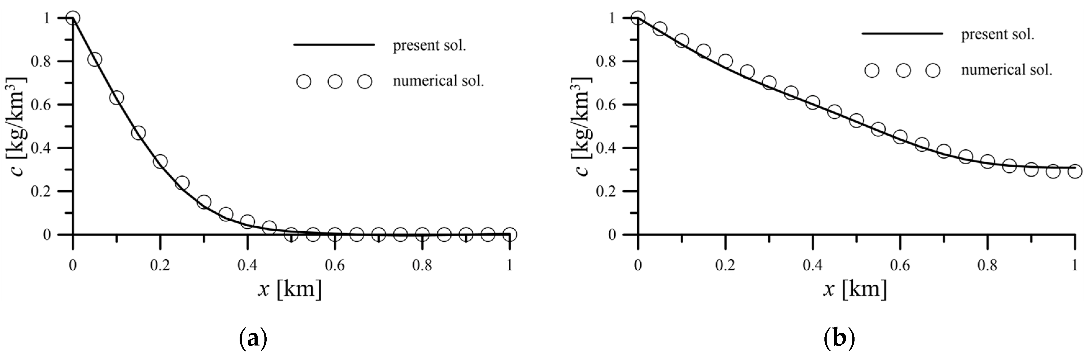
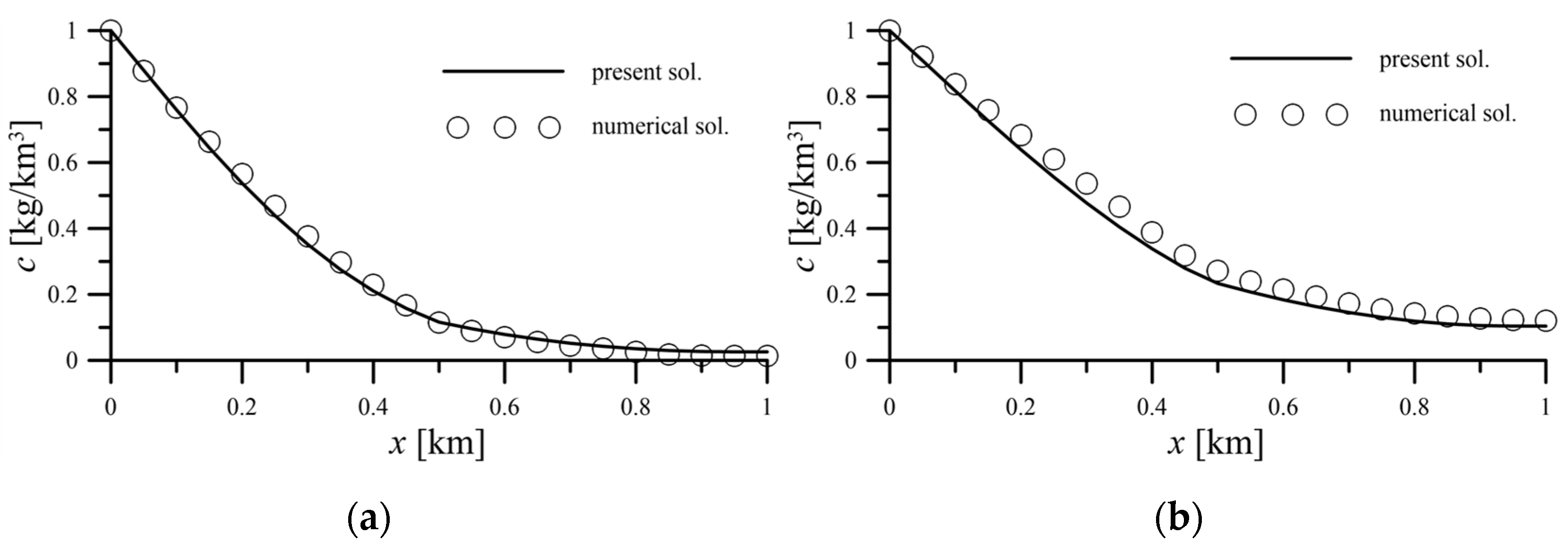
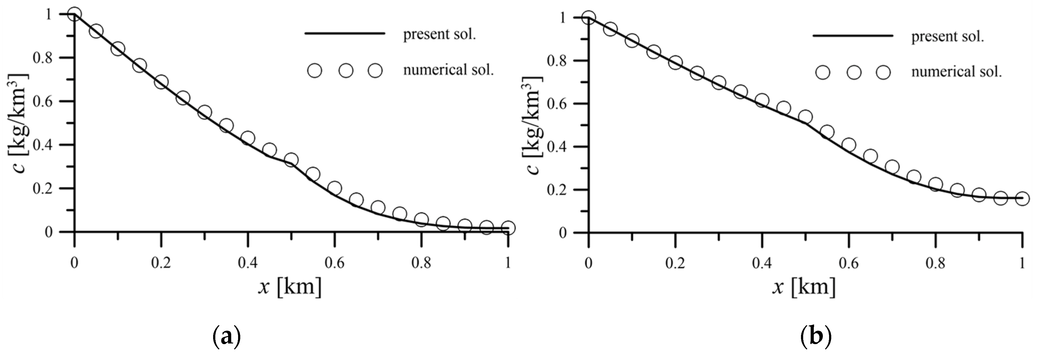
In order to verify this analytical solution, we used a numerical solution for verification. Figure 3 is the comparison of analytical solutions and numerical solutions in the case of one-zoned homogeneous soil in a finite field. It can be seen from Figure 3 that the analytical results with simulation time of 0.1 year and 1 year are consistent with the results of the numerical simulation. The parameters are referred to Kumar et al. [4], assuming $L=1 \mathrm{km}, D=0.21{ \mathrm{km}}^2/\mathrm{y}, V=0.11 \mathrm{km}/\mathrm{y}$.

Dispersion is due to the heterogeneity of porous media at the microscopic scale, leading to differences in groundwater flow path and average velocity and leading to solute dispersion. We set the soil zone to have different dispersion coefficients $D_1$ and $D_2$ and used the numerical solution to verify the analytical solution of the solute concentration transport in the two-zoned aquifer. The results are shown in Figure 4 and Figure 5. Figure 4 is the simulation result of the dispersion coefficient $D_1=0.1{ \mathrm{km}}^2/\mathrm{y}$ for $x=0–0.5 \mathrm{km}$ and the dispersion coefficient $D_2=0.2 {\mathrm{km}}^2/\mathrm{y}$ for $x=0.5–1 \mathrm{km}$, respectively for 0.5 years and 1 year. Figure 5 is the simulation result of the dispersion coefficient $D_1=0.2 {\mathrm{km}}^2/\mathrm{y}$ for $x=0–0.5 \mathrm{km}$ and the dispersion coefficient $D_2=0.1 {\mathrm{km}}^2/\mathrm{y}$ for $x=0.5–1 \mathrm{km}$, respectively, for 0.5 and 1 year. It can be seen from the figure that there is no significant difference between the analytical solution and the numerical solution.

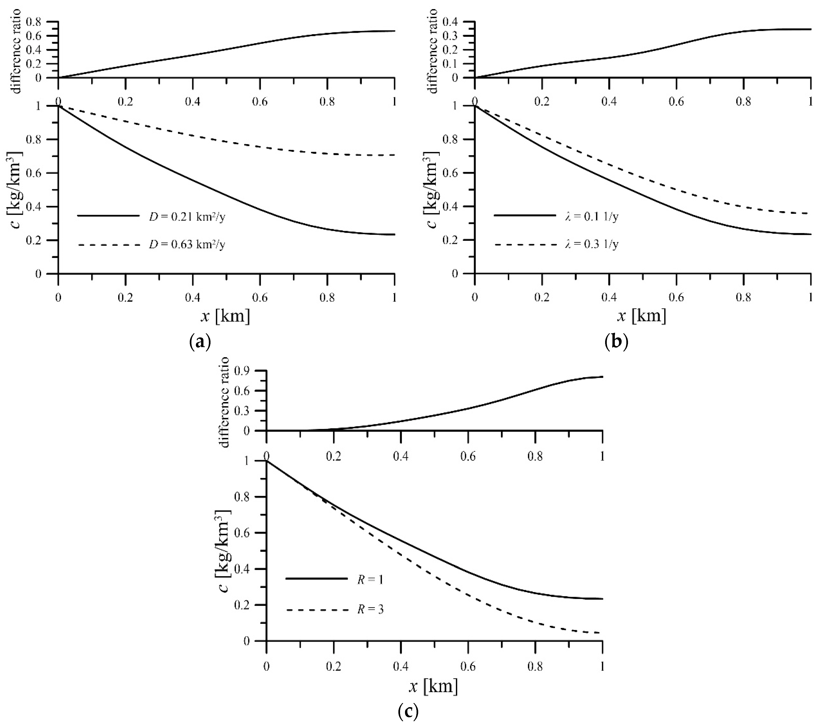
To understand the effect of each parameter on the change of solute concentration, we conducted the sensitivity analysis of relevant parameters, and the results are shown in Figure 6. By checking the difference ratio, when the dispersion coefficient, biodegradation factor, and retardation factor were all increased by 3 times, the difference ratio in the dispersion coefficient and retardation factor was relatively large. These two parameters have a greater influence on the change of solute concentration (Figure 6a,c). Conversely, the difference ratio of the biodegradation factor (Figure 6b) was only about 1/2 of that for the dispersion coefficient and retardation factor. The solute concentration was less sensitive to the biodegradation effect.

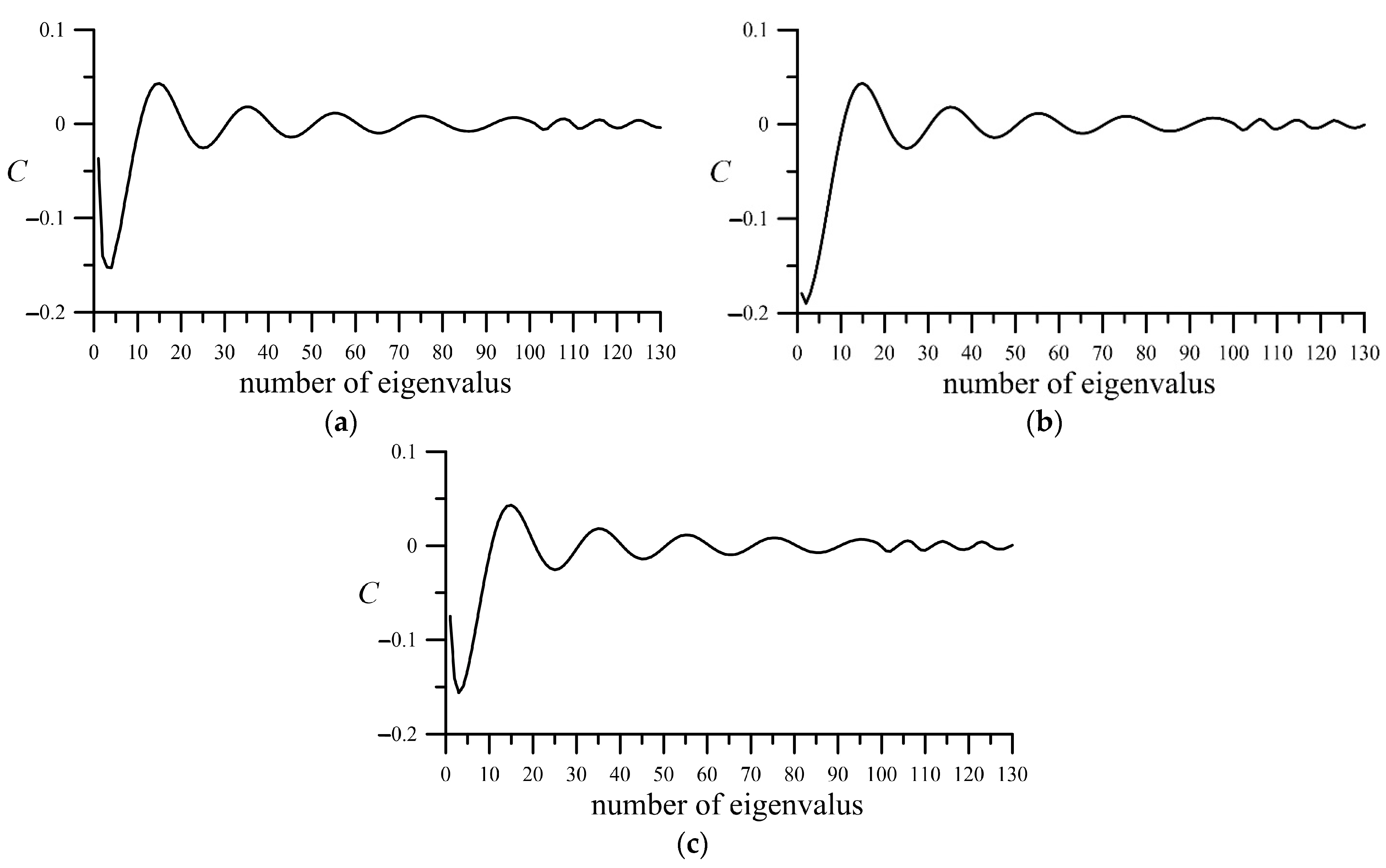
When using a generalized integral transform to solve boundary value problems, the number of eigenvalue terms will affect the convergence speed of the analytical solution. In the processes of deriving the analytical solution of solute transport in two-zoned media, the change-of-variable technique must be needed to eliminate the first order spatial differential term to comply with the requirement of applying the generalized integral transforms. In the inverse integral transform, an infinite series is included. Theoretically, the infinite series needs to be accumulated to a maximum number of terms in the calculations to reach a best accuracy of the solute concentration, but the summation could be stopped if the required accuracy is reached. Therefore, it is necessary to analyze and discuss the convergence behavior of this series. As shown in Figure 7, when the number of eigenvalues is less than 20, the solute concentration fluctuates greatly, about ±15%, and the analytical solution should be regarded as not converging yet. When the number of eigenvalues is between 20 and 60, the fluctuation of solute concentration is reduced to within ±5%, which is within an acceptable error range in engineering. At this time, the analytical solutions can be regarded as convergent. When the number of eigenvalues becomes larger than 60, the change in solute concentration is less than ±1%. At this time, it does not make much sense to continue to increase the number of eigenvalues. Conversely, the parameter will also have an impact on the number of eigenvalues required for the analytical solution to be convergent. Figure 7 shows the concentration variation for the Peclect number $\alpha$ = 0.0524, 0.524, and 5.24. It can be seen from the figure that when the number of eigenvalues is less than 20, $\alpha$ has a greater impact on the convergence of the analytical solution. However, when the number exceeds 20, the change of $\alpha$ is not meaningful for the convergence of the analytical solution. This study discusses the number of cumulative terms for the convergence of this series in different situations under the criteria of 10⁻³ (dimensionless).

4. Discussions

The variation of solute concentration is affected by dispersion coefficients, biodegradation factors, and retardation factors over time and space. The analysis of influence of these factors was reported and discussed here by performing the present mathematical model.

Microorganisms in natural soil and groundwater can self-decompose specific pollutants and convert themselves into substances that are harmless to the environment, which is called biodegradation. This study considers the first-order decay rate of pollutants to be constant, which can be converted from the pollutant half-life. When the first-order decay rate is zero, Equation (41) can be reduced to Equation (22). Figure 8 shows the variation of solute concentration over time and space with and without considering the biodegradable effect. This figure reveals that regardless of whether biodegradation is considered or not, the solute concentration will reach a stable concentration if the distance is long enough. As expected, the concentration considering biodegradation will be smaller than that without biodegradation effect.

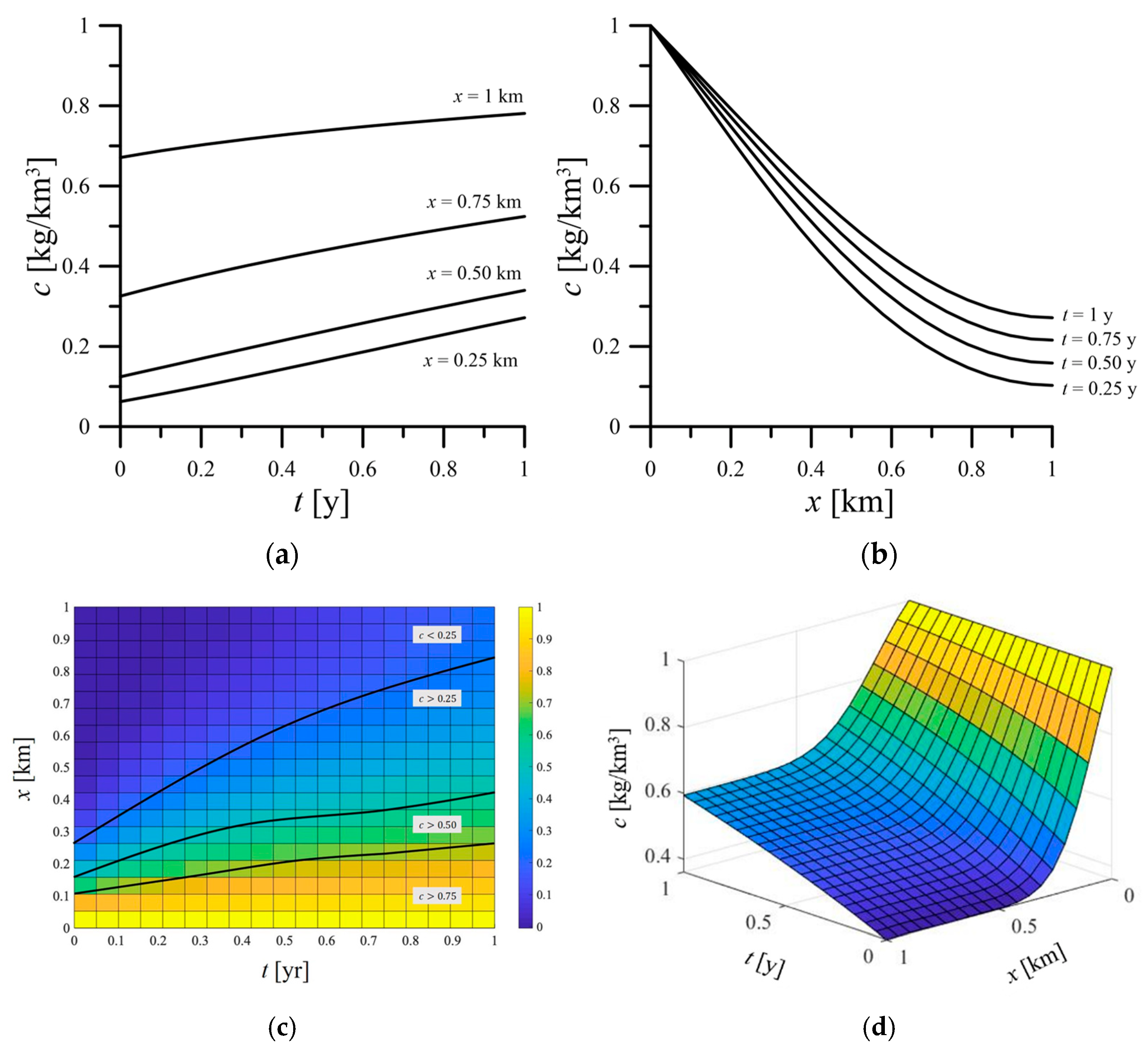
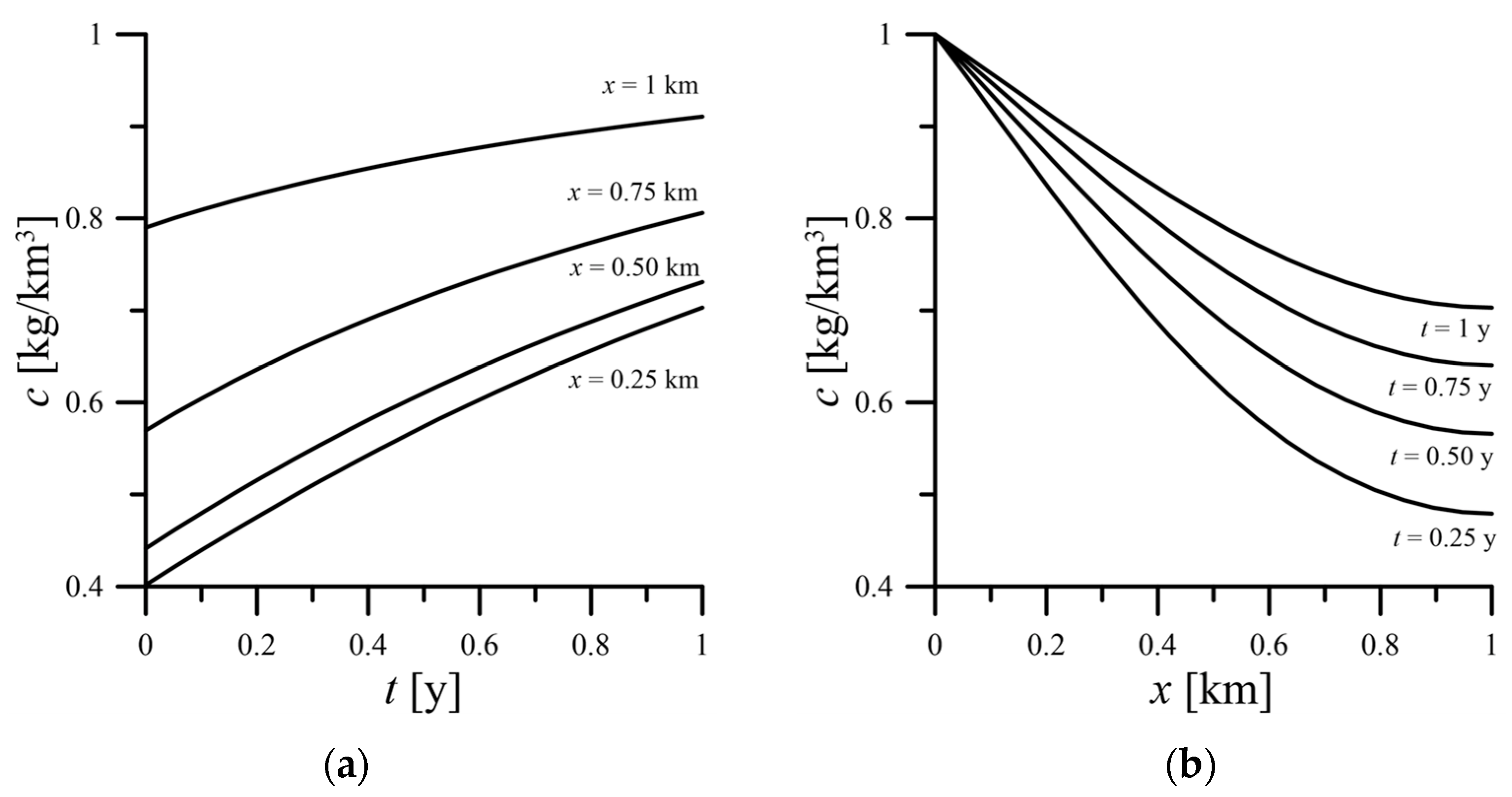
The one-zone solute transport simulation case in this study considers both retained and non-retained biodegradation effects, referring to Equations (1) and (23), and analytical solutions, Equations (22) and (41). Figure 9 shows how the solute concentration changes over time and space when considering the biodegradable effect. 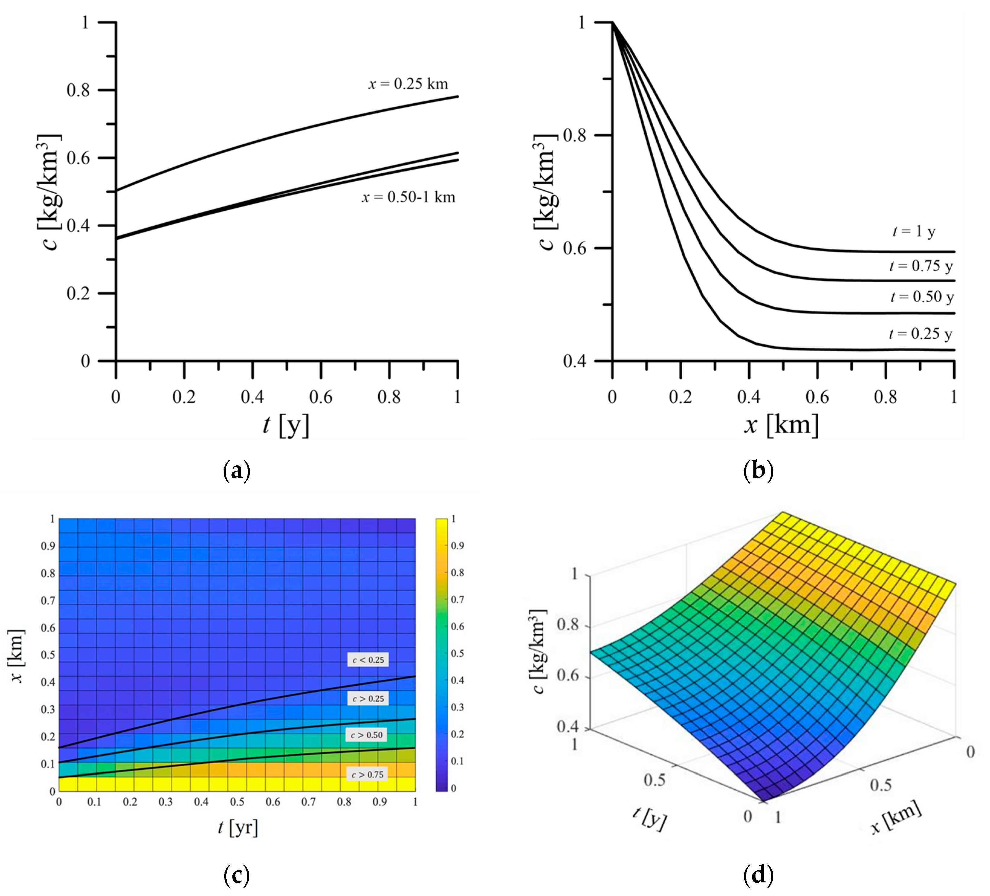The transport processes of the dimensionless solute concentration with the biodegradable effect are clearly shown in Figure 9c. All the local changes of the solute concentration will temporarily increase but will gradually become stable. 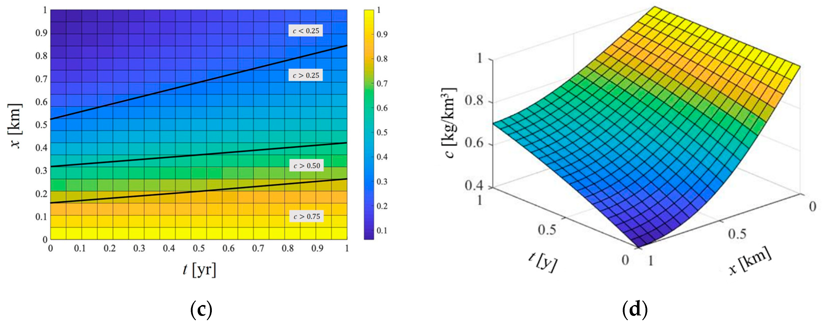When the biodegradable effect is not considered, the variations of solute concentration over time and space are shown in Figure 10. The concentration increases slowly from a higher initial value for different locations (Figure 10a,c) and decays slowly to a higher value over space at a certain duration (Figure 10b,c). Comparing Figure 9 and Figure 10, under the same simulation time of 1 year, the stable solute concentration without biodegradable effect is about 0.7 kg/km³, and the stable solute concentration with a biodegradable effect is about 0.3 kg/km³. The area of c < 0.50 kg/km³ becomes smaller and the other two areas of c > 0.50 kg/km³ and c > 0.75 kg/km³ become larger when the biodegradable effect is not considered. This clearly displays the effect of the biodegradation on the solute concentration, meaning that the biodegradable effect has an apparent effect on the solute concentration distribution.

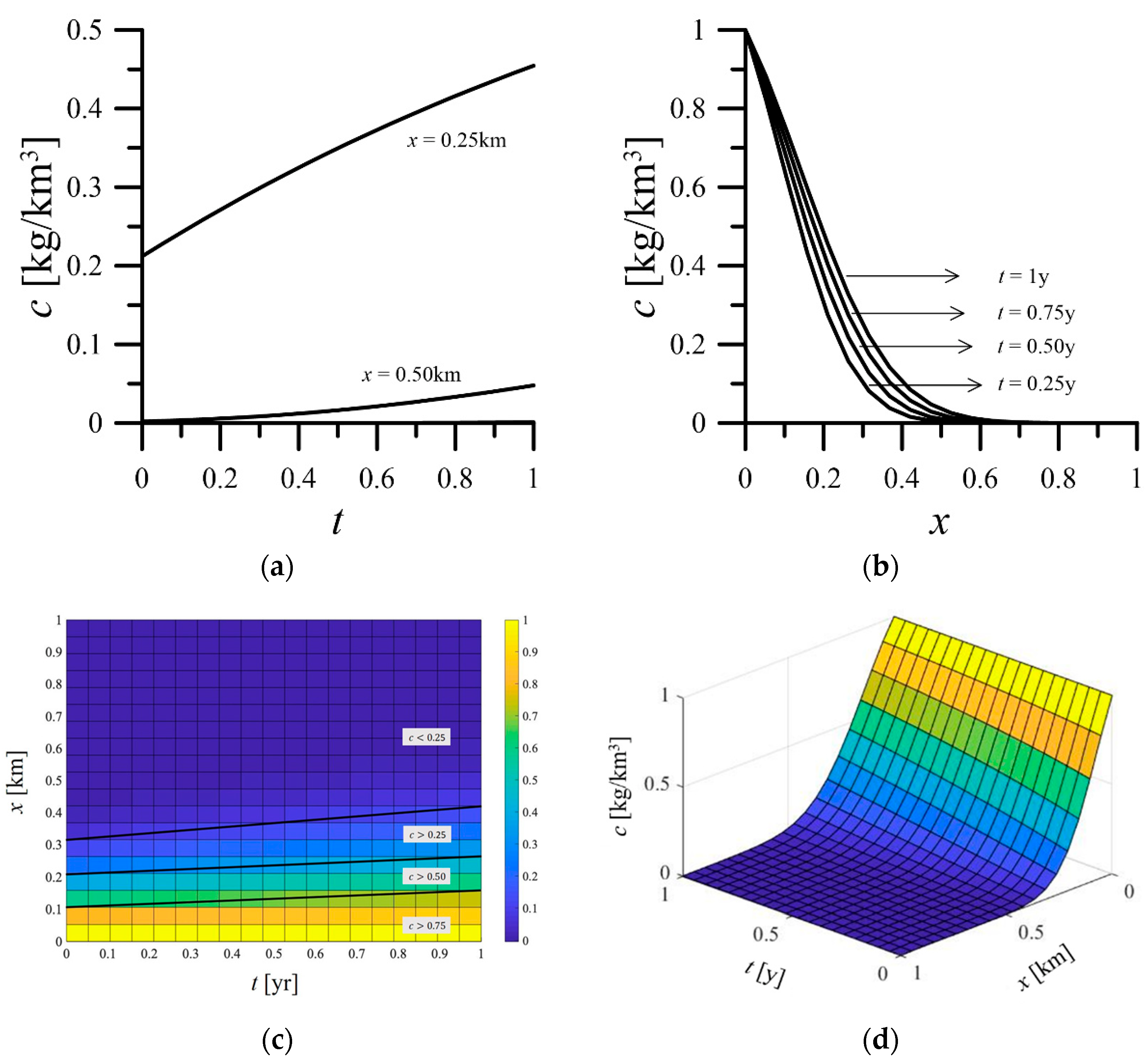
The parameters used in Figure 11 are $L=1 \mathrm{km}, D=0.021{ \mathrm{km}}^2/\mathrm{y}, V=0.11 \mathrm{km}/\mathrm{y}$, which describes the slower transport rate of solute in the aquifer. From the figure, when the biodegradable effect is considered, the solute concentration tends to stabilize with the increase of time and space. In addition, because of the low solute transport speed and the influence of the biodegradable effect, the solute concentration approaches zero at about x $\ge$ 0.6 km. In other words, the solute is completely degraded. Therefore, no concentration will be observed at any location x $\ge$ 0.6 km before 1 year.

). (a) The solute concentration varies with time. (b) The solute concentration varies with space. (c) The change of solute concentration over time and space. (d) 3D plot of solute concentration change over time and space.

The same parameters are used in Figure 12 but without considering the biodegradable effect. From the figure, the solute concentration increases with time. The increase of the concentration is also quite insignificant after the position of x = 0.5 km. Because the biodegradable effect is not considered, the solute concentration reaches different stable values for different stages. When compared with Figure 11, although the concentration variation in Figure 12 has the same trend, the concentration can still be observed over the space, and the concentration c is larger than 0.40 kg/km³ for the hypothetical cases at different durations.

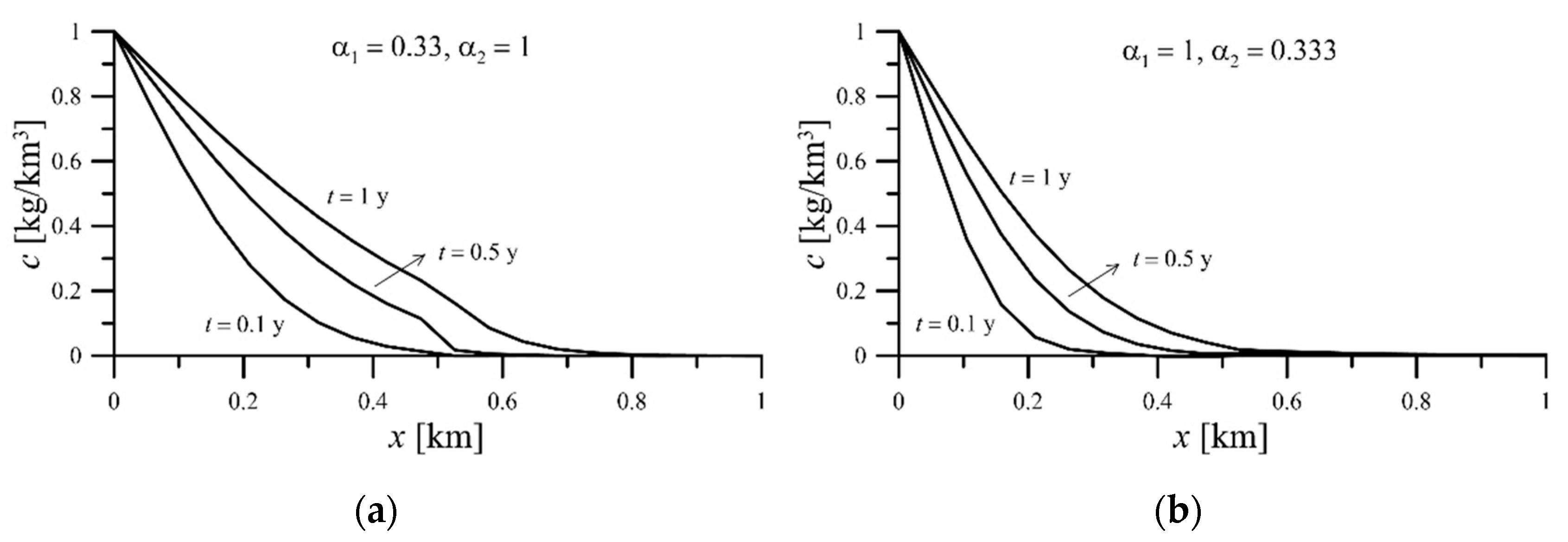
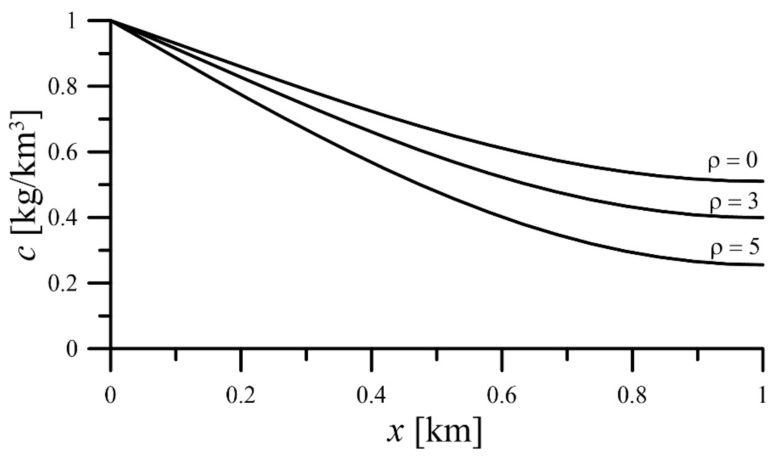
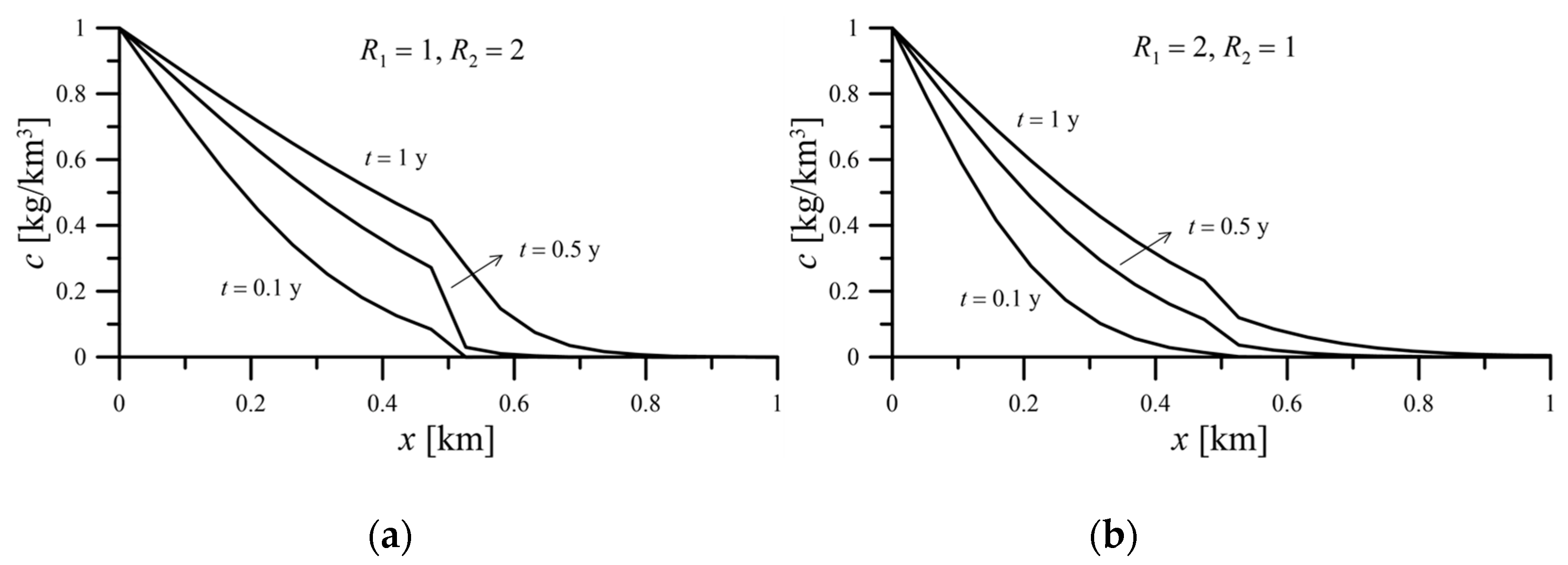
Conversely, Figure 13 shows the spatial distribution of contaminated concentrations in the composite aquifer for different Peclect numbers. When ${\alpha }_1<{\alpha }_2$ (Figure 13a), the contaminated concentration decreases gradually with increasing distance in zone 1. As $x\ge 0.5 \mathrm{km}$, the concentration first drops quickly and then decreases gradually because of the smaller Peclect number. Oppositely, when ${\alpha }_1>{\alpha }_2$ (Figure 13b), the variation of contaminated concentration drops fast in zone 1 because of the larger Peclect number. The effect of different Peclect numbers on the change of contaminated concentration is especially obvious for a longer period. The concentration variation at the interface of the composite aquifer becomes smooth for ${\alpha }_1>{\alpha }_2$ because the concentration decays to a low value at the interface, and thus the transport flux has no effect on it.

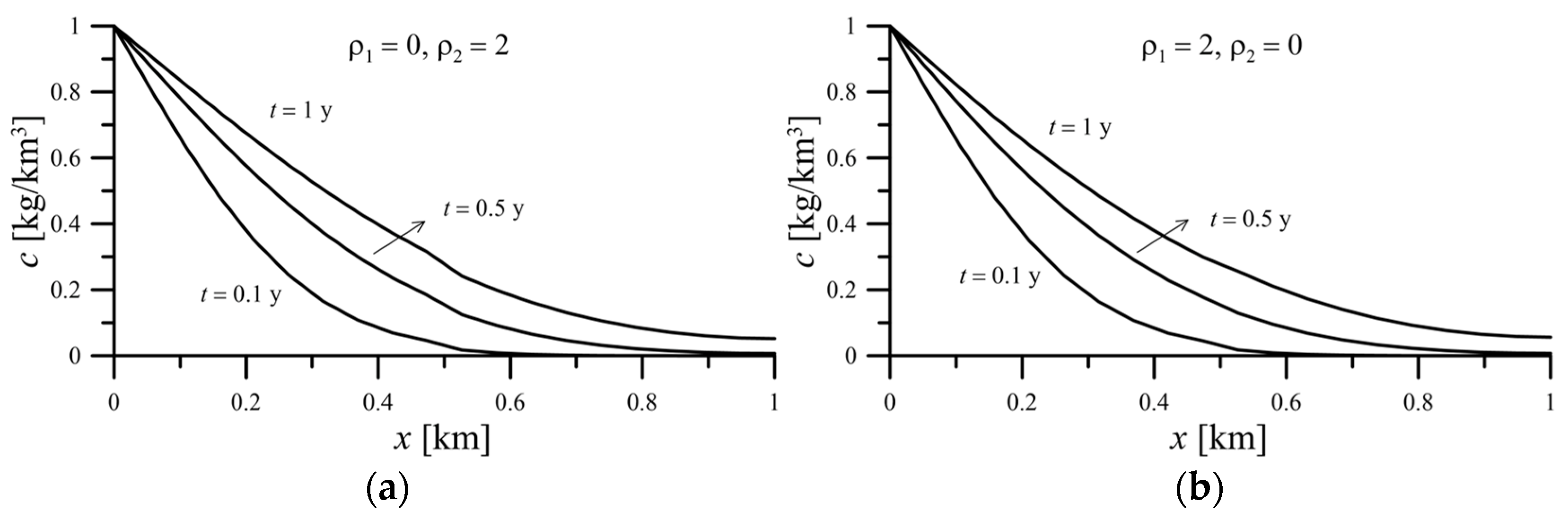
The adsorption factor is usually considered in combination of various gases or dissolved pollutants and the surface of solid materials. In the groundwater system, solid matter such as the aquifer medium or sandy soil and the pollutant is in the dissolved phase. This phenomenon will affect the solute concentration in the porous medium. In this study, the adsorption phenomenon only considers linear equilibrium adsorption by introducing a retardation factor. Figure 14 compares the effect of the retardation factor on the solute concentration. For a larger adsorption factor, the solute concentration decays more quickly. Therefore, the change of solute concentration decreases fast in zone 2 in Figure 14a but in zone 1 in Figure 14b. It was noted that the solute concentration at the interface drops more quickly in Figure 14a than in Figure 14b because of the higher retardation effect.

During the transport of solute concentrations, the factors such as Peclect number ($\alpha$) and retardation factor (R) directly affect the solute concentration in a short period. However, the biodegradation factor ($\rho$) is a biological and chemical effect, which lasts for a long time but has less influence than the Peclect number ($\alpha$) and retardation factor (R). Figure 15 reveals that the solute concentration increases with time at every location and decreases gradually over the distance at any duration. Notably, the influence of biodegradation factors on the change of solute concentration is not significant, regardless that ${\rho }_1>{\rho }_2$ or ${\rho }_1<{\rho }_2,$ but the concentration gradient near the interface of the two zones slightly changes for ${\rho }_1<{\rho }_2$ when the duration is greater than one year.

From the above modeling of the concentration of solute transport, it was found that in a composite aquifer, the decaying and diffusion (in the Peclect number) factors have an apparent effect on the contaminated concentration at the interface, especially for long-term modeling.

5. Conclusions

Analytical solutions to ADEs of the solute transport in groundwater flow under the hypothetical scenario designed as an aquifer between a landfill field and a permeable reactive barrier are presented and verified with numerical solutions. The presented exact solutions are obtained by the generalized integral transform method associated with change-of-variables technique. Further, the modeling results indicate that the present mathematical model is an efficient tool to model or predict the variation of contamination concentration for a groundwater flow in a two-zoned aquifer, which can be extended to an n-zoned aquifer in the future. Some remarkable points are summarized as follows:

(1)

An analytical solution for solute transport in vertically layered geological media is derived by employing GITM. Owing to the existence of an infinite series in the analytical solution, the convergence precision should be checked via counting the number of eigenvalues to make sure that the solution is correct.

(2)

The contaminated concentration decreases as the retardation factor, Peclect number, and the first-order decaying coefficient increase for every location at a fixed duration. Moreover, the contaminated concentration is more sensitive to the Peclect number than to the retardation factor and the first-order decaying coefficient in uniform groundwater flow. The effects of decaying and diffusion factors on the contaminated concentration around the interface become apparent over a long-term period.

(3)

In nature, aquifers are usually composite. The present mathematical model can be applied to simulate or predict the transport of the pollutant concentration in groundwater flow in a single-layered aquifer and a two-zoned aquifer. Further, this model can be extended to a more complex model considering an n-zoned porous medium to study their solute transport in groundwater flow in the future.

References

1. Schuetz, T.; Weiler, M.; Lange, J.; Stoelzle, M. Two-dimensional assessment of solute transport in shallow waters with thermal imaging and heated water. Adv. Water Resour. 2012, 43, 67–75. [Google Scholar] [CrossRef]
2. Rubol, S.; Battiato, I.; de Barros, F.P.J. Vertical dispersion in vegetated shear flows. Water Resour. Res. 2016, 52, 8066–8080. [Google Scholar] [CrossRef]
3. Fry, V.A.; Istok, J.D.; Guenther, R.B. An analytical solution to the solute transport equation with rate-limited desorption and decay. Water Resour. Res. 1993, 29, 3201–3208. [Google Scholar] [CrossRef]
4. Kumar, A.; Jaiswal, D.K.; Kumar, N. Analytical solutions of one-dimensional advection-diffusion equation with variable coefficients in a finite domain. J. Earth Syst. Sci. 2009, 118, 539–549. [Google Scholar] [CrossRef] [Green Version]
5. Kumar, A.; Jaiswal, K.; Kumar, N. Analytical solutions to one-dimensional advection–diffusion equation with variable coefficients in semi-infinite media. J. Hydrol. 2010, 380, 330–337. [Google Scholar] [CrossRef]
6. Néelz, S. Limitations of an analytical solution for advection-diffusion with spatially variable coefficients. Commun. Numer. Methods Eng. 2005, 22, 387–396. [Google Scholar] [CrossRef]
7. Jaiswal, D.K.; Kumar, A.; Kumar, N.; Yadav, R.R. Analytical solutions for temporally and spatially dependent solute dispersion of pulse type input concentration in one-dimensional semi-infinite media. J. Hydro-Environ. Res. 2009, 2, 254–263. [Google Scholar] [CrossRef]
8. Jaiswal, D.K.; Kumar, A.; Yadav, R.R. Analytical solution to the one-dimensional advection-diffusion equation with temporally dependent coefficients. J. Water Resour. Prot. 2011, 3, 76–84. [Google Scholar] [CrossRef] [Green Version]
9. Liang, X.; Zhang, Y.-K.; Liu, J.; Ma, E.; Zheng, C. Solute transport with linear reactions in porous media with layered structure: A semi-analytical model. Water Resour. Res. 2019, 55, 5102–5118. [Google Scholar] [CrossRef]
10. Guerrero, J.P.; Pimentel, L.; Skaggs, T.; van Genuchten, M. Analytical solution of the advection–diffusion transport equation using a change-of-variable and integral transform technique. Int. J. Heat Mass Transf. 2009, 52, 3297–3304. [Google Scholar] [CrossRef]
11. Guerrero, J.P.; Skaggs, T. Analytical solution for one-dimensional advection–dispersion transport equation with distance-dependent coefficients. J. Hydrol. 2010, 390, 57–65. [Google Scholar] [CrossRef]
12. Jaiswal, D.K.; Kumar, A.; Kumar, N.; Singh, M.K. Solute Transport along Temporally and Spatially Dependent Flows through Horizontal Semi-Infinite Media: Dispersion Proportional to Square of Velocity. J. Hydrol. Eng. 2011, 16, 228–238. [Google Scholar] [CrossRef]
13. Schmid, B.H. On the transient storage equations for longitudinal solute transport in open channels: Temporal moments accounting for the effects of first-order decay. J. Hydraul. Res. 1995, 33, 595–610. [Google Scholar] [CrossRef]
14. Shukla, V.P. Analytical solutions for unsteady transport dispersion of nonconservative pollutant with time dependent periodic waste discharge concentration. J. Hydraul. Eng. 2002, 128, 866–869. [Google Scholar] [CrossRef]
15. Gureghian, A.B.; Jansen, G. One-dimensional analytical solutions for the migration of a three-member radionuclide decay chain in a multilayered geologic medium. Water Resour. Res. 1985, 21, 733–742. [Google Scholar] [CrossRef]
16. Leij, F.J.; van Genuchten, M.T. Approximate analytical solutions for solute transport in two-layer porous media. Transp. Porous Media 1995, 18, 65–85. [Google Scholar] [CrossRef]
17. Leij, F.J.; Skaggs, T.H.; van Genuchten, M.T. Analytical solution for solute transport in three-dimensional semi-infinite porous media. Water Resour. Res. 1991, 27, 2719–2733. [Google Scholar] [CrossRef]
18. Li, Y.-C.; Cleall, P.J. Analytical solutions for advective-dispersive solute transport in double-layered finite porous media. Int. J. Numer. Anal. Methods Geomech. 2011, 35, 438–460. [Google Scholar] [CrossRef]
19. Guerrero, J.P.; Pimentel, L.; Skaggs, T. Analytical solution for the advection–dispersion transport equation in layered media. Int. J. Heat Mass Transf. 2012, 56, 274–282. [Google Scholar] [CrossRef]
20. Batu, V. A generalized two-dimensional analytical solute transport model in bounded media for flux-type finite multiple sources. Water Resour. Res. 1993, 29, 2881–2892. [Google Scholar] [CrossRef]
21. Chen, J.-S.; Ni, C.-F.; Liang, C.-P.; Chiang, C.-C. Analytical power series solution for contaminant transport with hyperbolic asymptotic distance-dependent dispersivity. J. Hydrol. 2008, 362, 142–149. [Google Scholar] [CrossRef]
22. van Genuchten, M.T.; Alves, W.J. Analytical Solutions of the One-Dimensional Convective-Dispersive Solute Transport Equation; US Department of Agriculture, Agricultural Research Service: Ohio, OH, USA, 1982; p. 1661. [Google Scholar]
23. Chen, J.-S.; Ni, C.-F.; Liang, C.-P. Analytical power series solutions to the two-dimensional advection-dispersion equation with distance-dependent dispersivities. Hydrol. Process. 2008, 22, 4670–4678. [Google Scholar] [CrossRef]
24. Park, E.; Zhan, H. Analytical solutions of contaminant transport from finite one- two three-dimensional sources in a finite-thickness aquifer. J. Contam. Hydrol. 2001, 53, 41–61. [Google Scholar] [CrossRef]
25. Chen, J.-S.; Lai, K.-H.; Liu, C.-W.; Ni, C.-F. A novel method for analytically solving multi-species advective–dispersive transport equations sequentially coupled with first-order decay reactions. J. Hydrol. 2011, 420–421, 191–204. [Google Scholar] [CrossRef]
26. Wu, M.-C.; Hsieh, P.-C. Improved Solutions to the Linearized Boussinesq Equation with Temporally Varied Rainfall Recharge for a Sloping Aquifer. Water 2019, 11, 826. [Google Scholar] [CrossRef] [Green Version]
27. Özisik, M.N. Boundary Value Problems of Heat Conduction; Dover Publications, Inc.: New York, NY, USA, 1968. [Google Scholar]
Figure 1. Schematic of this study.
Water 14 00323 g001
Figure 2. The flow chart of derivation of the analytical solution.
Water 14 00323 g002
Figure 3. Validation of present solutions with numerical solutions for the one-zone model. The black line denotes the analytical solution and the circle denotes the numerical solution. (a) t = 0.1   y , (b) t = 1   y .
Water 14 00323 g003
Figure 4. Validation of present solutions with numerical solution, D 1 = 0.1   km 2 / y ,   D 2 = 0.2   km 2 / y for the two-zone model. The black line denotes the analytical solution and the circle denotes the numerical solution. (a) t = 0.5   y , (b) t = 1   y .
Water 14 00323 g004
Figure 5. Validation of present solutions with numerical solution, D 1 = 0.2   km 2 / y ,   D 2 = 0.1   km 2 / y for the two-zone model. The black line denotes the analytical solution and the circle denotes the numerical solution. (a) t = 0.5   y , (b) t = 1   y .
Water 14 00323 g005
Figure 6. Comparison of solute concentration under different (a) dispersion coefficients, (b) biodegradation factors, (c) retardation factors.
Water 14 00323 g006
Figure 7. The influence of the number of eigenvalues and the Peclect number on solute concentration. (a) α = 0.0524 , (b) α = 0.524 , (c) α = 5.24 .
Water 14 00323 g007
Figure 8. Variation of contaminated concentration for different first-order decaying coefficients.
Water 14 00323 g008
Figure 9. The change of solute concentration when the influence of biodegradation is considered. ( D = 0.21   km 2 / y ,   R = 1 ,   λ = 0.1 / y ) . (a) The solute concentration varies with time. (b) The solute concentration varies with space. (c) The change of solute concentration over time and space. (d) 3D plot of solute concentration change over time and space.
Water 14 00323 g009
Figure 10. The change of solute concentration when the influence of biodegradation is not considered. ( D = 0.21   km 2 / y ,   R = 1 ,   λ = 0 . (a) The solute concentration varies with time. (b) The solute concentration varies with space. (c) The change of solute concentration over time and space. (d) 3D plot of solute concentration change over time and space.
Water 14 00323 g010aWater 14 00323 g010b
Figure 11. The change of solute concentration when the influence of biodegradation is considered. ( D = 0.021   km 2 / y ,   R = 1 ,   λ = 0.1 / y . (a) The solute concentration varies with time. (b) The solute concentration varies with space. (c) The change of solute concentration over time and space. (d) 3D plot of solute concentration change over time and space.
Water 14 00323 g011
Figure 12. The change of solute concentration when the influence of biodegradation is not considered. ( D = 0.021   km 2 / y ,   R = 1 ,   λ = 0 ). (a) The solute concentration varies with time. (b) The solute concentration varies with space. (c) The change of solute concentration over time and space. (d) 3D plot of solute concentration change over time and space.
Water 14 00323 g012
Figure 13. Spatial variation of contaminated concentrations in a composite aquifer.   ( R = 1 ,   λ = 0.1 ) . (a) α 1 < α 2 (b) α 1 > α 2 .
Water 14 00323 g013
Figure 14. Spatial variation of contaminated concentrations in a composite aquifer. ( D = 0.21   km 2 / y ,   λ = 0.1 ). (a) R 1 < R 2 (b) R 1 > R 2 .
Water 14 00323 g014
Figure 15. Variation of contaminated concentrations for different first-order decaying coefficients. ( D = 0.21   km 2 / y ,   R = 1 ) . (a) ρ 1 < ρ 2 (b) ρ 1 > ρ 2 .
Water 14 00323 g015
Publisher’s Note: MDPI stays neutral with regard to jurisdictional claims in published maps and institutional affiliations.