Time-Discrete Hedging of Down-and-Out Puts with Overnight Trading Gaps

Abstract

Hedging down-and-out puts (and up-and-out calls), where the maximum payoff is reached just before a barrier is hit that would render the claim worthless afterwards, is challenging. All hedging methods potentially lead to large errors when the underlying is already close to the barrier and the hedge portfolio can only be adjusted in discrete time intervals. In this paper, we analyze this hedging situation, especially the case of overnight trading gaps. We show how a position in a short-term vanilla call option can be used for efficient hedging. Using a mean-variance hedging approach, we calculate optimal hedge ratios for both the underlying and call options as hedge instruments. We derive semi-analytical formulas for optimal hedge ratios in a Black–Scholes setting for continuous trading (as a benchmark) and in the case of trading gaps. For more complex models, we show in a numerical study that the semi-analytical formulas can be used as a sufficient approximation, even when stochastic volatility and jumps are present.

1. Introduction

This paper analyzes time-discrete hedging of European down-and-out put options near the barrier in the case of overnight trading gaps. Such barrier options are not only traded over-the-counter, but are also embedded in certain types of retail derivatives, for example, bonus certificates (Baule and Tallau 2011; Baule and Shkel 2021; Hernández et al. 2008), bonus certificates plus (Hernández and Liu 2014), flex bonus certificates (Hernández et al. 2014) or (multi) barrier reverse convertibles (Wallmeier and Diethelm 2009). In these markets, banks act as market makers and continuously quote prices for their issued products during trading hours. Adequate hedging procedures that can also take overnight trading gaps into account are therefore highly relevant.

The payoff of down-and-out put options is discontinuous at the barrier, which make the use of a classical delta hedging problematic when the underlying level approaches the barrier. This is why some approaches suggest hedging exotic options by using a static portfolio of vanilla options that replicates the exotic payoff at maturity and is zero in case of a barrier hit.1 However, to set up a perfect static hedge, a continuum of vanilla options would be required. Engelmann et al. (2006) show with empirical data that certain static hedge strategies for down-and-out puts outperform a delta hedge in a local volatility model, while others are worse. Tompkins (2002) shows in a simulation study that neither dynamic hedging nor static hedging leads to satisfactory results for up-and-out calls and that the variability of hedging error is even higher for the static approach than delta hedging. It is also possible to try combining static and dynamic hedging (İlhan and Sircar 2006; İlhan et al. 2008; Leung and Lorig 2015). Maruhn and Sachs (2009) developed static superreplication hedging techniques that are robust regarding the underlying model parameters. The biggest challenge, however, is the need to simultaneously unwind the entire hedge portfolio when the barrier is breached. Even robust techniques may lead to very high hedging errors when this is not possible, for example, in the case of trading gaps Maruhn et al. (2011).

Another strand of literature considers delta hedging for more complex models. An and Suo (2009) compare the performance of delta-hedging up-and-out calls on FX rates for several underlying processes, featuring stochastic volatility and jumps. However, they consider hedging errors as averages over the whole lifespan of many up-and-out calls. In this paper, we focus on the hedging situation close to the barrier. One might argue that the problems of a classical delta hedge can be diminished when the hedging frequency is increased near the barrier. However, this is only possible when the underlying is traded continuously. On real equity markets, trading hours are restricted, and the barrier can be breached over night, when there is no chance to take action.2 Furthermore, stock prices may be subject to discontinuous jumps, even during regular trading hours, e.g., (Ait-Sahalia and Jacod 2009; Cont and Tankov 2004; Cont 2001; Kou 2007). We therefore consider both regular overnight jumps and stochastic jumps in our analysis.

Even for vanilla options, a classical delta hedge, based on the derivative of the contingent claim value with respect to the underlying price, may lead to considerable hedging errors when hedging is performed in discrete time intervals. Therefore, recent research has focused on methods to calculate a minimum variance delta for vanilla options that takes a discrete hedging period into account (Alexander et al. 2012; Hull and White 2017; Vähämaa 2004). Nian et al. (2018) use a market-data-driven approach, applying kernel functions to determine a delta that minimizes a quadratic empirical loss function in discrete time. However, market data of options are needed for this approach, which is not attainable for exotic options. Schweizer (2001) and Pham (2000) have proposed mean-variance hedging, using self-financing strategies that minimize the mean squared error (MSE) between the contingent claim at maturity and the terminal hedge portfolio value. We also use a mean-variance hedging strategy, but minimize the MSE for a short period (one day) rather than until maturity. We thus focus on the most crucial hedging situation, when the underlying is already close to the barrier and a knock out event is likely to occur.

Similar to our approach, Bemporad et al. (2010, 2014) use a stochastic model predictive control technique to minimize the variance of the hedging portfolio at a discrete future point in time. Bemporad et al. (2011) and Graf Plessen et al. (2019) include the squared expected hedging error in addition to the hedging variance in their optimization. As a major extension, we analyze the situation of trading gaps. In general, hedging errors can be computed using Monte Carlo simulation techniques. We consider (i) a geometric Brownian motion for the underlying, (ii) a jump diffusion process, and (iii) a model with stochastic volatility and jumps. Beyond simulation techniques, we additionally derive semi-analytical formulas in the Black–Scholes case.

We add to the literature on hedging barrier options by analyzing the most difficult situation of down-and-out puts close to the barrier in the presence of overnight trading gaps. As our main contribution, we show that the existence of trading gaps has a significant impact on mean-variance optimal hedge ratios compared to discrete hedging in continuous time. Furthermore, we introduce the idea of using opposite vanilla options to dynamically hedge barrier options (i.e., vanilla calls to hedge down-and-out puts).3 In a Black–Scholes framework (with and without trading gaps), we develop semi-analytical formulas for mean-variance optimal hedge ratios. A numerical analysis shows that mean-variance hedging leads to much smaller root mean squared errors (RMSE) and value-at-risk figures than classical delta hedging or static hedging. Hedging errors can become quite small when continuous trading is possible. However, when trading gaps are considered, hedging errors are much larger close to the barrier for all strategies. Using short-term vanilla call options as hedge instruments instead of the underlying can further significantly reduce RMSE. If it is possible to find a vanilla call that expires exactly after the trading gap, RMSE and value-at-risk can be reduced to almost zero.

Interestingly, these results also hold in more complex models, beyond geometric Brownian motion. Actually, there are virtually no differences between the results of a model with jumps and the Black–Scholes case.4 This finding raises the question of whether the comparably simple semi-analytical formulas can yield reasonable results in more complicated situations. Indeed, such an approach—assuming geometric Brownian motion although the actual process is different—leads to fairly small hedging errors, despite the not correctly specified model. Therefore, practitioners might use the semi-analytical approach even when the underlying process is more complex than a geometric Brownian motion.

The remainder of this paper is structured as follows: Section 2 describes the hedging problem and our approach for down-and-out puts and provides a total of seven different hedging strategies. These include no hedging, time-continuous Black–Scholes delta hedging, one static approach as well as mean-variance delta hedging using the underlying or vanilla calls with different maturities. Section 3 shows the results of a numerical analysis of hedging errors using the aforementioned strategies in the Black–Scholes model. Semi-analytical formulas for the mean-variance optimal hedge ratios for the Black–Scholes model are derived. We distinguish between continuous trading and overnight gap risk during the hedge period in order to see the effect of including trading gaps on hedging errors. In Section 4, we extend the underlying model and allow for jumps and stochastic volatility. After presenting the similar results in the jump-diffusion case, we calculate hedging errors when the semi-analytical formulas are applied in a model with stochastic volatility and jumps. Section 5 gives a short conclusion.

2. The Hedging Problem

2.1. Mean-Variance Hedging

We consider a European down-and-out put (dop) with strike price K, a barrier B that is continuously monitored during trading hours and maturity T. The underlying level at time t is denoted $S_t$. The payoff at maturity is given by

$$max(K-S_T,0){𝟙}_{\{S_t\ge B,\forall t\in [0,T]\}},$$

(1)

which means that the difference $K-S_T$ is only paid when both the underlying price is below the strike K at maturity and the barrier B has never been hit during the lifetime of the dop.

The main hedging difficulties arise from the discontinuity of the payoff at the barrier: the maximum payoff is reached just before the barrier and then drops to zero (see Figure 1, dotted black line). As the barrier hit probability increases when the underlying level approaches the barrier from above, the value of the down-and-out put before maturity decreases and reaches zero at the barrier (Figure 1, black line). Near the barrier, the likelihood of a barrier hit causes the time value to be negative and counteract the inner value $K-S_t$. Accordingly, the derivative of the value with respect to the underlying level—delta—is positive and very high just above the barrier. Delta becomes negative for higher underlying levels, similar to a vanilla put option, and is bounded from below by $-1$. Of course, delta is zero below the barrier. Delta is thus also discontinuous at the barrier (Figure 1, dashed black line).

In theory, hedging options with Black–Scholes delta leads to a perfect hedge when all corresponding assumptions are met. Hedging in such a way would also minimize the variance of the hedging portfolio (Bakshi et al. 1997). However, in reality, trading is only possible at discrete times and thus price changes are discrete, too. This is especially true when the exchange closes over night or at weekends. When the barrier is hit at the next trading instance, the down-and-out put is worthless. However, the hedger is still long in the underlying and faces corresponding losses. Consequently, the Black–Scholes delta might lead to large hedging errors. We therefore build a hedge portfolio consisting of ${\delta }_{MSE}^S$ positions of the underlying that minimizes the squared hedging error for a discrete hedging period $\mathsf{\Delta }t$,

$${\delta }_{MSE}^S = \underset{\delta }{arg\; min}\mathbb{E}{[\underset{=:\mathsf{\Delta }{f}_{\mathsf{\Delta }t}}{\underbrace{(f_{\mathsf{\Delta }t}-f_0{e}^{r\mathsf{\Delta }t})}}-\delta \underset{=:\mathsf{\Delta }{S}_{\mathsf{\Delta }t}}{\underbrace{(S_{\mathsf{\Delta }t}-S_0{e}^{r\mathsf{\Delta }t})}}|{\mathcal{F}}_0]}^2,$$

(2)

where $f_t$ denotes the price of the dop at time t.5 Without loss of generality, we set $t\equiv 0$. ${\mathcal{F}}_0$ is the information set at time zero. This approach is similar to the minimization of quadratic hedging errors, i.e., mean-variance hedging in incomplete markets, which was introduced by Föllmer and Sondermann (1986).6

Equation (2) explicitly refers to the underlying itself as the hedging instrument. However, there might be other liquidly traded instruments that are better suited. In particular, short-termed vanilla call options with a strike identical to the barrier of the down-and-out put option could be superior, as illustrated in Figure 1. For a vanilla call that matures at the end of the hedging period $\mathsf{\Delta }t$, its payoff below the barrier is zero, inducing a perfect hedge below the barrier. The steep positive slope of the down-and-out put above the barrier can be closely approximated by an appropriate number of vanilla calls. In practice, however, it is not always possible to find a vanilla call option that expires exactly at time $\mathsf{\Delta }t$. Nonetheless, vanilla calls with short maturities promise to be a better alternative to the underlying as the hedging instrument. We therefore extend the minimization problem (2) to call options with maturity $T_{call}$:

$${\delta }_{MSE}^{C^{T_{call}}} = \underset{\delta }{arg\; min}\mathbb{E}{[\mathsf{\Delta }{f}_{\mathsf{\Delta }t}-\delta \mathsf{\Delta }{C}_{\mathsf{\Delta }t}^{T_{call}}|{\mathcal{F}}_0]}^2,$$

(3)

where $\mathsf{\Delta }{C}_{\mathsf{\Delta }t}^{T_{call}}$ describes the price difference from $t=0$ to $t=\mathsf{\Delta }t$ of the corresponding vanilla call option.

According to Föllmer and Schweizer (1988, p. 151 ff.), using linear regression, the solution of (2) and (3) is given by

$${\delta }_{MSE}^H=\frac{Cov(\mathsf{\Delta }{f}_{\mathsf{\Delta }t},\mathsf{\Delta }{H}_{\mathsf{\Delta }t})}{Var\left(\mathsf{\Delta }{H}_{\mathsf{\Delta }t}\right)}=\frac{Cov(f_{\mathsf{\Delta }t},H_{\mathsf{\Delta }t})}{Var\left(H_{\mathsf{\Delta }t}\right)},$$

(4)

with the hedge instrument $H\in \{S,C^{T_{call}}\}$. Moreover, the hedging error is zero in expectation. In Section 3, we show how this representation can be used to derive semi-analytical formulas in a Black–Scholes setting.

2.2. Hedging Situation and Strategies

In our numerical analysis, we consider a down-and-out put with strike $K=100$ and barrier $B=80$. As the delta near the barrier increases when maturity comes closer, we choose a fairly small remaining lifetime of $T=20$ days. For the hedging period, we set $\mathsf{\Delta }t=1$ day, as it is common practice to adjust the hedging portfolio on a daily basis. A Monte Carlo simulation is used to generate prices of the underlying in $t+\mathsf{\Delta }t$ similar to Bemporad et al. (2014). In a first setting (Section 3), we consider the Black–Scholes model, assuming that the underlying follows a geometric Brownian motion. In a second setting (Section 4), we additionally consider stochastic volatility and especially jumps in the underlying process, because jump events may have a significant impact on the hedge variance.

For both settings, we analyze two different situations regarding the trading of the underlying: First, trading continues throughout the hedging period, and the barrier can be breached at any time between $t=0$ and $t=\mathsf{\Delta }t$. Second, there is no actual trading between $t=0$ and $t=\mathsf{\Delta }t$, and whether the barrier is breached or not depends solely on the underlying level at time $\mathsf{\Delta }t$. The second situation mimics the overnight gap risk between two trading days. While the usual overnight gap is shorter than one day, it is longer at weekends. One day is therefore a good proxy for an average trading gap.

As we are interested in the hedging performance near the barrier, we consider underlying levels $S_t$ between 80 and 82. For higher prices, it is less likely that a barrier event occurs within $\mathsf{\Delta }t$. Hence, standard hedging procedures may be applied in these cases. We investigate a total of seven different hedging strategies:

• Standard delta hedging with the underlying model;
• Static hedging with the strike spread approach of Carr and Chou (1997);
• Mean-variance hedging with ${\delta }_{MSE}^S$ obtained by (2) using the underlying;
• Mean-variance hedging with ${\delta }_{MSE}^{C^{T_{call}}}$ obtained by (3) using vanilla call options with the following maturities:

  (a)

  1 day (best case, when available);

  (b)

  5 days (normal case, weekly options are available for major stock indices);

  (c)

  20 days (worst case, time to maturity identical to dop).

• No hedging.

In Section 3, we show that hedging errors for the standard delta and static strike spread approach are nearly identical in our setting. That is why the latter is omitted in Section 4. We further only consider call options as hedge instruments that expire in one or five trading days in Section 4.2.

3. Hedging under Geometric Brownian Motion

3.1. Model and Parameters

In this section, we assume that the stock price follows a geometric Brownian motion, as in Black and Scholes (1973) and Merton (1973). The risk-neutral price dynamics of the underlying are given by

$$\frac{d{S}_t}{S_t}=rdt+{\sigma }_{BS}d{W}_t,$$

(5)

where W is a Wiener process, r is the risk-free rate, and ${\sigma }_{BS}$ is the volatility.

A major advantage of the Black–Scholes model is the availability of closed-form solutions for both vanilla European options and down-and-out put options. The price of a vanilla European call can be calculated as

$$C_{0,BS}^{T_{call}}=S_{0}N\left(d_1\right)-K{e}^{-r{T}_{call}}N\left(d_2\right),$$

(6)

where

$$\begin{array}{cc}\hfill d_1& =\frac{log(S_0/K)+(r+{\sigma }_{BS}^2/2)T_{call}}{{\sigma }_{BS}\sqrt{T_{call}}},\hfill \\ \hfill d_2& =d_1-{\sigma }_{BS}\sqrt{T_{call}}.\hfill \end{array}$$

The price of a down-and-out put option is given by the Reiner and Rubinstein (1991) formula:

$$\begin{array}{cc}\hfill f_0^{BS}\left(S_0\right)=& -S_{0}N(-x_1)+K{e}^{-rT}N(-x_1+{\sigma }_{BS}\sqrt{T})\hfill \\ \hfill & +S_{0}N(-x_2)-K{e}^{-rT}N(-x_2+{\sigma }_{BS})\sqrt{T}\hfill \\ \hfill & -S_0{(B/S_0)}^{2(\mu +1)}N\left(y_1\right)+K{e}^{-rT}{(B/S_0)}^{2\mu }N(y_1-{\sigma }_{BS}\sqrt{T})\hfill \\ \hfill & +S_0{(B/S_0)}^{2(\mu +1)}N\left(y_2\right)-K{e}^{-rT}{(B/S_0)}^{2\mu }N(y_2-{\sigma }_{BS}\sqrt{T})\hfill \\ \hfill & +K\left({(B/S_0)}^{\mu +\lambda }N\left(z\right)+{(B/S_0)}^{\mu -\lambda }N(z-2\lambda {\sigma }_{BS}\sqrt{T})\right),\hfill \end{array}$$

(7)

where

$$\begin{array}{cccc}\hfill x_1& =\frac{log(S_0/K)}{{\sigma }_{BS}\sqrt{T}}+(1+\mu ){\sigma }_{BS}\sqrt{T}\hfill & \hfill y_1& =\frac{log(B^2/\left(S_{0}K\right))}{{\sigma }_{BS}\sqrt{T}}+(1+\mu ){\sigma }_{BS}\sqrt{T}\hfill \\ \hfill x_2& =\frac{log(S_0/B)}{{\sigma }_{BS}\sqrt{T}}+(1+\mu ){\sigma }_{BS}\sqrt{T}\hfill & \hfill y_2& =\frac{log(B/S_0)}{{\sigma }_{BS}\sqrt{T}}+(1+\mu ){\sigma }_{BS}\sqrt{T}\hfill \\ \hfill \mu & =\frac{r-{\sigma }_{BS}^2/2}{{\sigma }_{BS}^2}\lambda =\sqrt{{\mu }^2+\frac{2r}{{\sigma }_{BS}^2}}\hfill & \hfill z& =\frac{log(B/S_0)}{{\sigma }_{BS}\sqrt{T}}+\lambda {\sigma }_{BS}\sqrt{T}.\hfill \end{array}$$

We fix the risk-free rate at $r=0.01$ and the volatility at ${\sigma }_{BS}=0.2$.

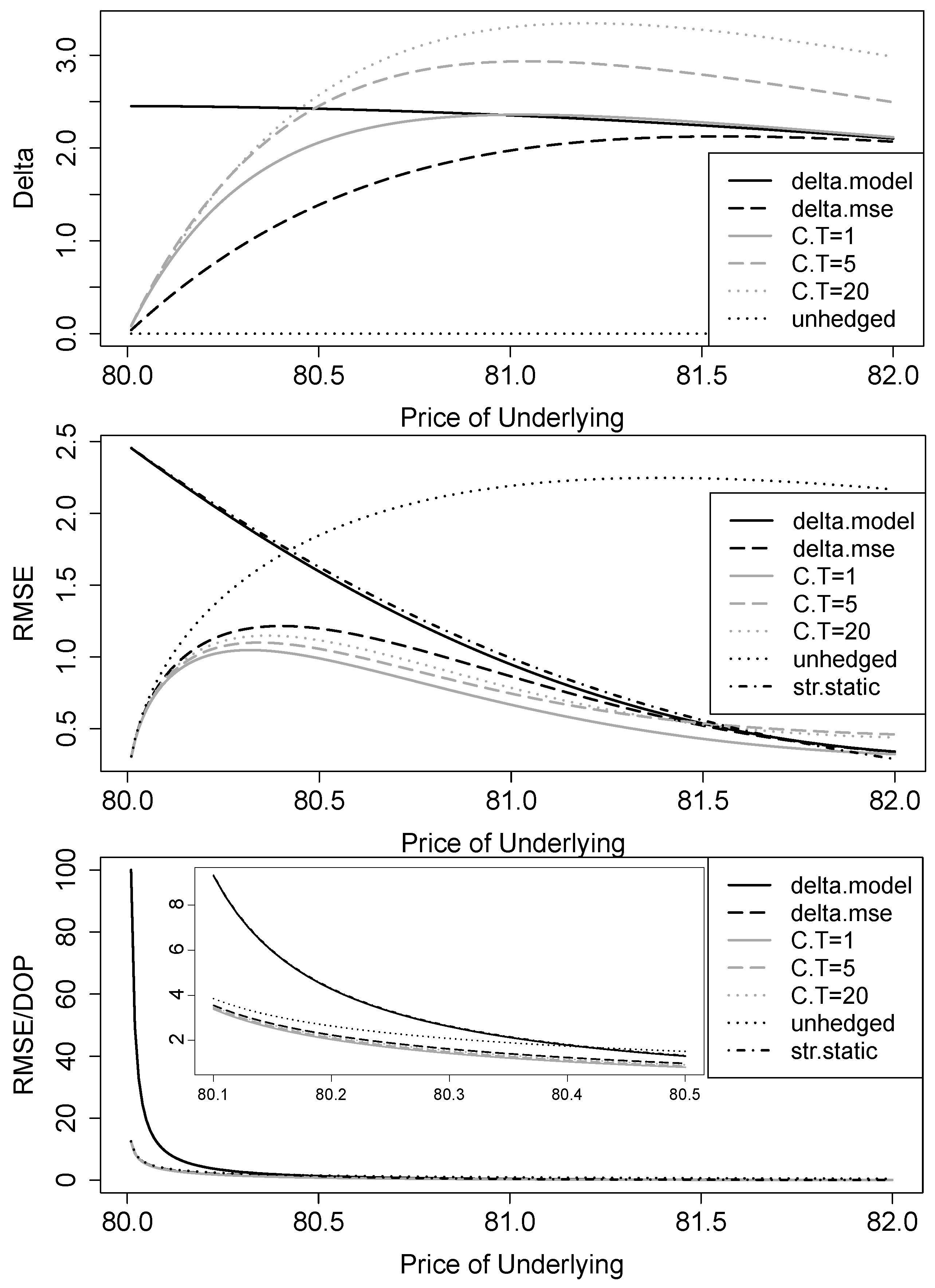
3.2. Continuous Trading

To see what effect overnight gap risk may have on hedging performance, we first consider the standard case when trading continues throughout the one-day hedging period. To apply the mean-variance hedge Equation (4), we need the Black–Scholes price of the dop and the hedge instrument at time $t=\mathsf{\Delta }t$. For an underlying price $S_{\mathsf{\Delta }t}$, we can apply Formula (7); however, we must consider the possibility that a barrier crossing took place between $t=0$ and $t=\mathsf{\Delta }t$. Given $S_0$ and $S_{\mathsf{\Delta }t}$, the probability that no barrier crossing occurs can be calculated via Brownian bridge calculus (e.g., Glasserman 2004) as

$$1-\pi \left(S_{\mathsf{\Delta }t}\right)=1-exp\left(\frac{-2log(S_0/B)·log(S_{\mathsf{\Delta }t}/B)}{{\sigma }_{BS}^2\mathsf{\Delta }t}\right).$$

(8)

The conditional expectation of the dop price at time $t=\mathsf{\Delta }t$, given $S_{\mathsf{\Delta }t}$, but with the information set ${\mathcal{F}}_0$ (without knowing the underlying path between $t=0$ and $t=\mathsf{\Delta }t$), is then given by

$$E\left(f_{\mathsf{\Delta }t}^{BS}\left(S_{\mathsf{\Delta }t}\right)\right|{\mathcal{F}}_0)=(1-\pi \left(S_{\mathsf{\Delta }t}\right))·f_{\mathsf{\Delta }t}^{BS}\left(S_{\mathsf{\Delta }t}\right).$$

(9)

To solve ${\delta }_{MSE}$ from Equation (4) semi-analytically, we write it in integral form:

$${\delta }_{MSE}^H=\frac{E(f_{\mathsf{\Delta }t}·H_{\mathsf{\Delta }t}|{\mathcal{F}}_0)-E\left(f_{\mathsf{\Delta }t}\right|{\mathcal{F}}_0)·E\left(H_{\mathsf{\Delta }t}\right|{\mathcal{F}}_0)}{E\left({\left(H_{\mathsf{\Delta }t}\right)}^2\right|{\mathcal{F}}_0)-E{\left(H_{\mathsf{\Delta }t}\right|{\mathcal{F}}_0)}^2}.$$

(10)

Defining the log returns of the underlying as $r_S:=log(S_{\mathsf{\Delta }t}/S_0)$ and expressing them in terms of standard normal variates z via $r_S\left(z\right)=(r-{\sigma }_{BS}^2/2)\mathsf{\Delta }t+{\sigma }_{BS}\sqrt{\mathsf{\Delta }t}z$, we obtain

$$E(f_{\mathsf{\Delta }t}^{BS}·H_{\mathsf{\Delta }t}|{\mathcal{F}}_0)={\int }_{y^{*}}^{\infty }(1-\pi (S_0·e^{r_S\left(z\right)}))f_{\mathsf{\Delta }t}^{BS}\left(S_0{e}^{r_S\left(z\right)}\right)H_{\mathsf{\Delta }t}\left(S_0{e}^{r_S\left(z\right)}\right)\varphi \left(z\right)dz,$$

(11)

where $\varphi (·)$ represents the normal density and the lower bound $y^{*}$ is

$$y^{*}=\frac{logB/S_t-(r-{\sigma }_{BS}^2/2)\mathsf{\Delta }t}{{\sigma }_{BS}\sqrt{\mathsf{\Delta }t}}.$$

(12)

The other integrals are calculated analogously, also mean and root mean squared hedging errors.7

Figure 2 shows the hedge ratios and absolute and relative root mean squared error (RMSE) for the seven hedging strategies, dependent on the current price of the underlying for a discrete one-day hedge of a down-and-out put with barrier $B=80$, strike price $K=100$ and 20 days to maturity. The hedge ratio of a classical Black–Scholes delta hedge reaches a value of about $2.5$ near the barrier. In contrast, hedge ratios for all mean-variance approaches become smaller and tend to zero when the price of the underlying approaches the barrier from above. The reason is that the probability of a barrier crossing becomes very high close to the barrier, and a high delta would lead to a large hedging error in the event of a barrier break. Figure 3 visualizes the barrier-hit probabilities, dependent on the underlying price. This probability also explains why the mean-variance deltas and the Black–Scholes delta converge for higher underlying prices, where barrier breaks are very unlikely within the hedging period. Looking at absolute RMSEs, the Black–Scholes delta and the static approach are virtually identical and lead to the highest errors of all strategies, with a maximum of $2.45$ at $S_0=80.01$. When the probability of hitting the barrier within the hedging period is very high, even the no-hedging strategy results in smaller errors than a standard delta hedge (at underlying prices of 80.50 and below). The best hedging results can be achieved by the mean-variance strategies with a hedging error of $0.30$ at $S_0=80.01$. As all mean-variance deltas are very small, the main driver of the hedging error is now the rare event when the dop is not knocked out. While using the 1-day vanilla call results in the best performance, the differences to the other mean-variance strategies are not as large. As long as the barrier-hit probability exceeds $20\%$ (at underlying levels below $81.50$), all mean-variance strategies outperform the standard delta and the static hedge. Relative RMSEs explode close to the barrier and take values of up to 100 for the standard delta and static hedge and values of 12 for the other strategies. However, since the RMSE is scaled by the price of the down-and-out put, which tends to zero as the underlying price reaches the barrier, these values are of little relevance here.

To provide further insight into the distribution of the hedging error and the risks involved, Figure 4 shows the relative hedge error distribution for an initial underlying level $0.5\%$ above the barrier ($S_0=80.40$). The figure furthermore depicts the relative 95% value at risk (VaR) for a long and a short hedge, respectively, depending on the initial underlying level $S_0$. The standard delta hedge and the static hedge result in a very fat-tailed and fairly symmetric error distribution. In contrast, the no-hedging distribution is positively skewed. This is because the hedge error is bounded by $100\%$ in the case of a barrier event and unbounded otherwise. All mean-variance strategies except for the 1-day vanilla call are more leptocurtic; however, they lead to less extreme hedge error in all cases. The error distribution with the 1-day call has both a high concentration around zero as well as the least amount of extreme errors.

Regarding relative VaR, it is important to distinguish whether a long or a short dop is hedged. The reason is the different source of high errors. If a long position is hedged, high errors occur when the barrier is hit during the hedging period. In this case, no hedging actually yields the best result, as the maximum loss is the value of the dop (100%). The Black–Scholes delta and the static hedge yield extreme relative VaRs of more than 10,000% and are therefore not shown in Figure 4. Compared to these extreme values, all MSE strategies yield significant improvements. Interestingly, for underlying prices of $80.5$ and below, the hedge with the underlying outperforms the hedges with the vanilla calls. In contrast, in the more relevant case for practice where a short position is hedged, high errors occur when the barrier is not hit. Here, the MSE hedges with vanilla calls result in best performances. However, differences between the MSE strategies are small unless the hedge is initiated only a few cents away from the barrier. As before, Black–Scholes delta and static hedging VaRs are extreme and therefore not plotted.

To sum up, all mean-variance strategies significantly outperform the Black–Scholes delta and static hedging when a dop is discretely hedged in continuous time. Comparing different mean-variance strategies, using call options as a hedge instrument instead of the underlying can further improve hedging performance, with shorter call option maturities to be preferred.

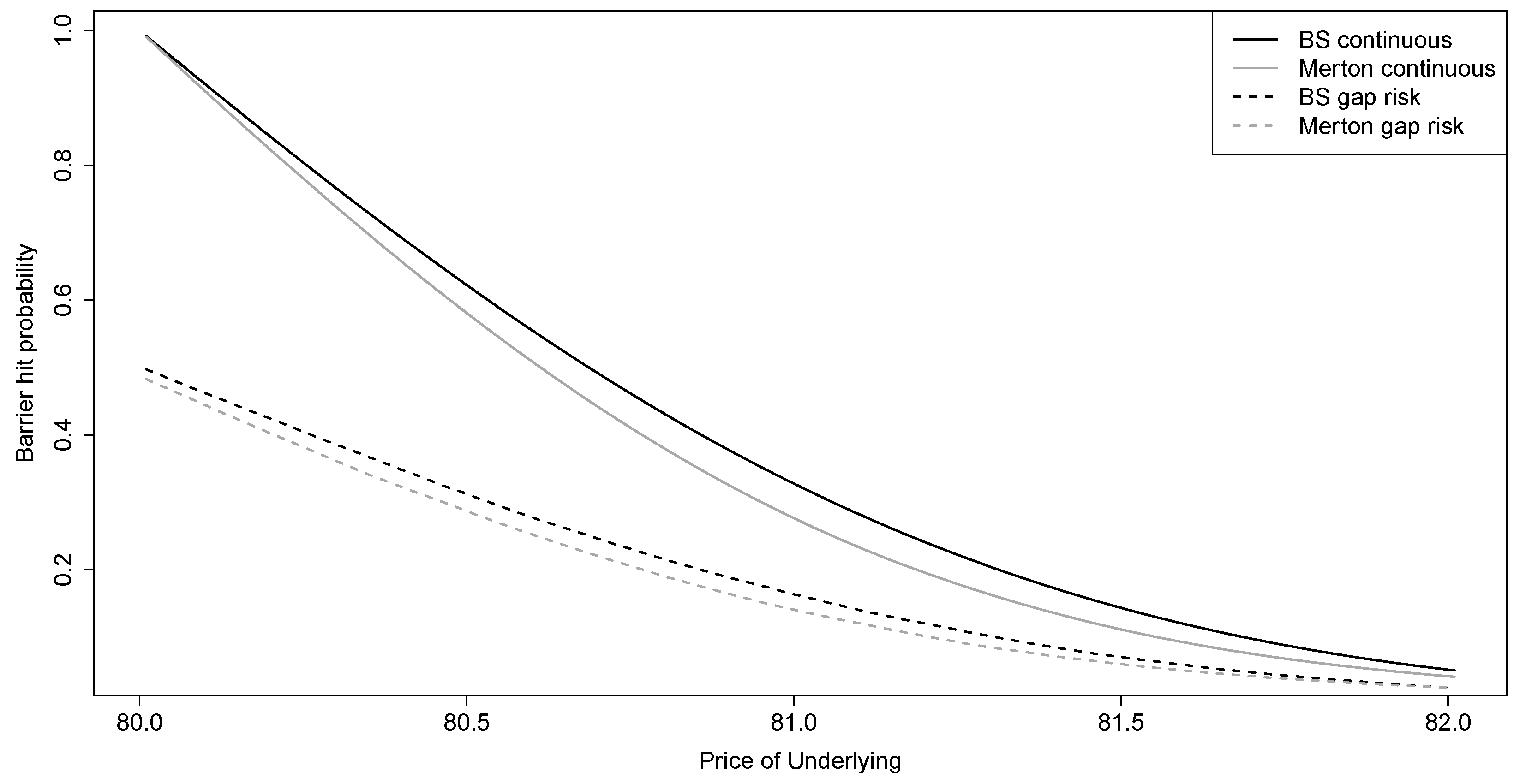
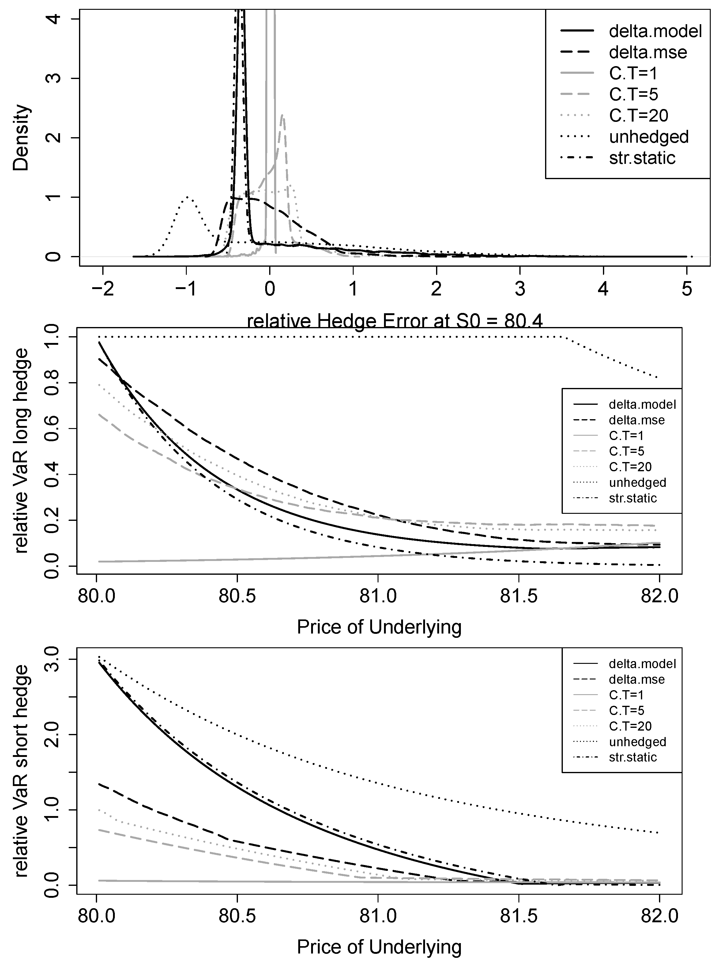
3.3. Overnight Trading Gaps

We now turn to the case, where there is no trading and thus no barrier observation during the hedging period. This is the situation when the hedger sets up the hedging portfolio before the exchange closes and the next chance to react will be on the following business day. We assume the overnight trading gap to be one calendar day, which is larger than the actual closing period between two regular days but smaller than the weekend closing period.

For valuation purposes, we assume continuous trading after the overnight gap at $t=\mathsf{\Delta }t$. We can thus proceed almost analogously to the continuous case to calculate semi-analytical solutions for ${\delta }_{minRMSE}$ in a world with overnight gap risk.8 However, we cannot use the Reiner and Rubinstein (1991) formula to calculate the dop value at $t=0$ immediately before the exchange closes, because this formula assumes a continuously monitored barrier—also during the overnight gap between $t=0$ and $t=\mathsf{\Delta }t$. This assumption would lead to an overestimation of knock outs: If the underlying price is extremely close to the barrier, the knock-out probability would tend to one under continuous trading. However, when the underlying closes one cent above the barrier, it has a fair chance of jumping over night to a level high above the barrier which makes a breach less likely. Figure 3 shows the probability of barrier crossings between $t=0$ and $t=\mathsf{\Delta }t$ with respect to $S_0$. An overnight gap reduces the knock-out probability and thus increases the value of the down-and-out put. In order to get a fair price for the down-and-out put, we use the approach of Baule et al. (forthcoming), discounting the expected value of the dop at the beginning of the next trading day.

Figure 5 summarizes the results for hedge ratios and absolute and relative RMSEs for the different strategies in the case of a trading gap within the one-day hedging period. The main difference to the continuous world from the previous section is that now hedge ratios of the mean-variance strategies do not tend to zero near the barrier. This is because now the down-and-out put value in $t=0$ is significantly higher than in a continuous setting because barrier-hit probabilities are much lower (about 50% compared to almost 100%; see Figure 3). The mean-variance delta using the underlying is still smaller than the Black–Scholes delta and has its minimum at $1.24$ compared to the Black–Scholes delta of $2.45$ at an underlying price of $80.01$. ${\delta }_{MSE}^{C^{1day}}$ for call options that mature at the end of the hedging period of one day is almost identical to the Black–Scholes delta. This is also plausible, because the most problematic scenario when $S_{\mathsf{\Delta }t}$ is below B yields a hedging error of zero, since both the call option and the down-and-out put have no payoff. For $S_{\mathsf{\Delta }t}>B$, the option delta is exactly one and thus yields the same precision as the Black–Scholes delta for the “good” case of no barrier break event. ${\delta }_{MSE}^{C^{5days}}$ and ${\delta }_{MSE}^{C^{20days}}$ are somehow larger, because deltas of these options are less than one, so more options are needed to eliminate the same amount of price risk.

Using mean-variance hedging with the underlying instead of the standard delta or the static approach cuts RMSE nearly by half close to the barrier, while the advantage diminishes at higher prices. Using the 1-day vanilla call is by far the best strategy in terms of RMSE. While it yields the same result far from the barrier as Black–Scholes delta or static hedging, the error close to the barrier is very low compared to the alternatives (only $0.05$, which is a $96\%$ RMSE reduction). The longer termed vanilla calls still lead to improved performances near the barrier. Interestingly, even absolute RMSEs for the 1-day call are smaller than in the world without gap risk. The reason for this is that on average the value of a dop in $t=0$ in the gap-risk world is higher than in the continuous world as barrier hits are less likely (see Figure 3). Deltas are thus higher, resulting in smaller hedging errors when no barrier event occurs. Finally, it is never advisable to completely forgo hedging, as no hedging results in the highest RMSE even close to the barrier, which is another difference to the continuous case.

Regarding relative RMSEs, errors increase for all strategies at underlying prices closer to the barrier. An exception is the 1-day call, which always yields a relative RMSE of only $5\%$, regardless of $S_0$. Because of higher dop values near the barrier, relative RMSE values tend to be smaller with trading gaps than with continuous trading.

Analogously to Figure 4, Figure 6 shows the distribution of relative hedging errors for a hedge initiated at $S_0=80.40$ as well as relative VaR values for long and short hedging. In general, distributions tend to be more skewed than in the continuous world. Regarding the modal values, there is a clear shift depending on the hedging strategy. Whereas no hedging results in a negative mode, the mode of the 1-day call strategy is nearly zero, while the 5-day and the 20-day calls yield positive modes. In addition, the distributions of the no-hedging, the Black–Scholes delta, and the static-hedging strategies have fat tails and are heavily skewed to the right.

Relative VaR for a long hedge is bounded above by 100% (for the no-hedging strategy). All other strategies yield fairly similar results; only the 1-day call leads to a significant VaR advantage.

As expected, short hedging is more associated with larger VaR values than long hedging. Additionally, the differences between hedging strategies are more severe for short positions close to the barrier. At $S_0=80.01$, the mean-variance hedge with the underlying reduces VaR already from 2.95 to 1.34. With vanilla options, the 5-days call can again halve this figure to $0.73$, and the 1-day call reduces VaR to only $0.06$.

3.4. Other Parameters

The price of a down-and-out put is higher near the barrier for a shorter time to maturity and also when the difference between strike and barrier is larger. For this reason, we rerun our calculations for a time to maturity of five days (instead of 20 days) and with a strike of 160 (strike-barrier ratio of 2 compared to $1.25$ for a strike of 100). While absolute hedge ratios and RMSEs increase, the relative RMSEs and relative densities and VaR figures are similar and have the same magnitudes. Relative hedge errors are also consistent for different levels of volatility. Hence, results are robust for different parameters and do not depend on the actual values considered for our in-depth analysis. Furthermore, since there was almost no difference between the Black–Scholes delta and the strike-spread static hedge, we skip the latter one in all further investigations.

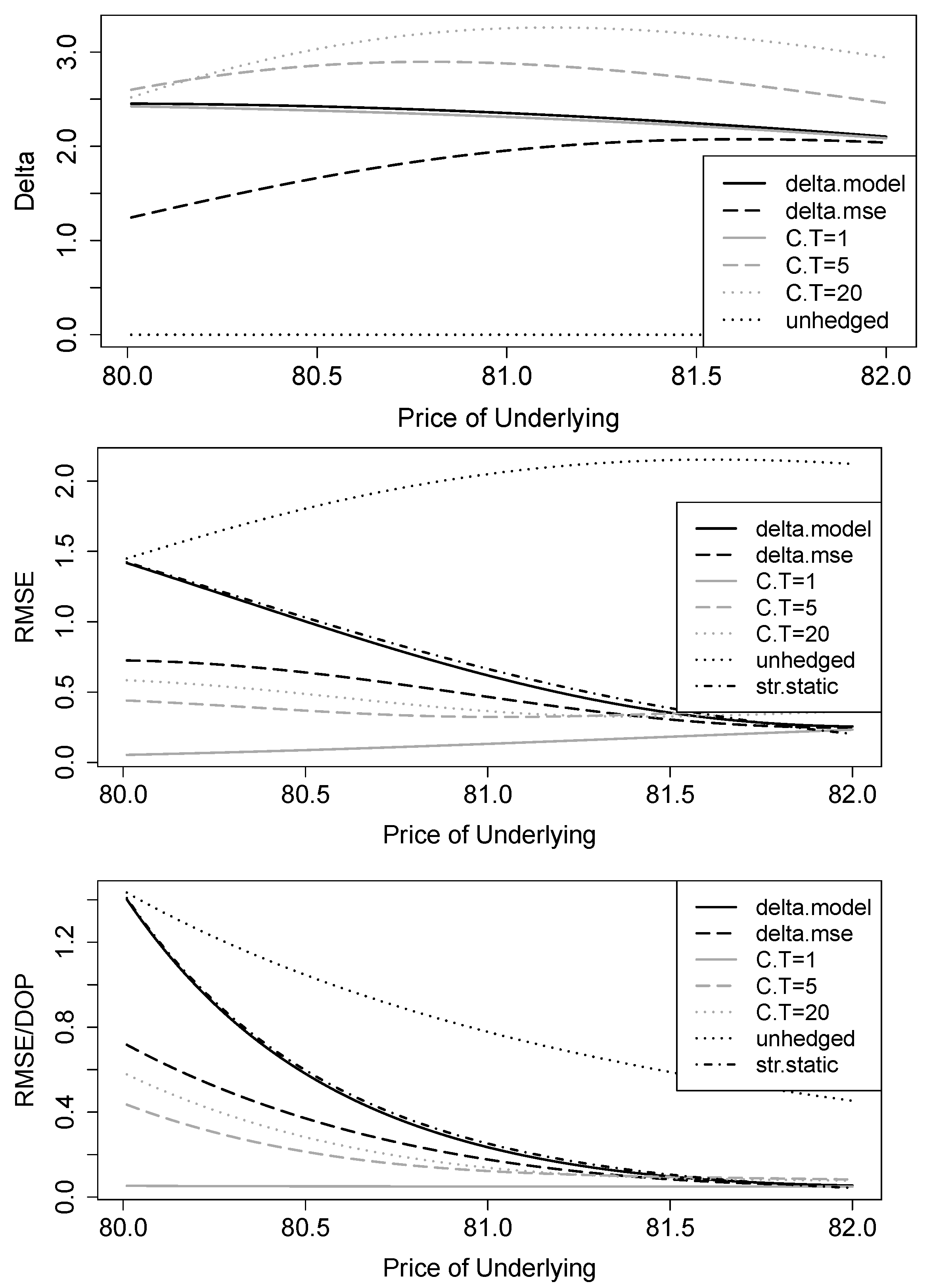
4. Robustness for Other Underlying Processes

4.1. Jump-Diffusion Model

It is widely accepted that the Black–Scholes model with log-normal underlying returns cannot accurately describe the empirically observed distribution (Cont 2001; Kou 2007). Most crucial for the performance of hedging approaches is the continuity of the process. In this section, we therefore allow stock prices to jump, applying the model of Merton (1976). Within this, the underlying follows a jump-diffusion process as follows:

$$\frac{d{S}_t}{S_t}=(r-{\lambda }_J{\mu }_J)dt+{\sigma }_{JD}d{W}_t+J_{t}d{N}_t,$$

(13)

where r is the risk free rate, ${\sigma }_{JD}$ is the volatility conditional on no jumps, $W_t$ is a Wiener process, and $N_t$ is a Poisson counting process with intensity ${\lambda }_J$. $J_t$ describes i.i.d. random jumps with distribution $log(1+J_t)\sim N(log(1+{\mu }_J-\frac{{\sigma }_J^2}{2}),{\sigma }_J^2)$, with two additional parameters ${\mu }_J$, ${\sigma }_J$.

A closed-form solution is only available for vanilla European options, while exotic options, such as the down-and-out put, must be evaluated numerically. A European call option can be calculated as a weighted sum of BS calls as follows:

$$C_{0,JD}^{T_{call}}=\sum _{i=0}^{\infty }\frac{exp(-(1+{\mu }_J){\lambda }_J){\left((1+{\mu }_J){\lambda }_J\right)}^i}{i!}{C}_{0,B{S}_i}^{T_{call}},$$

(14)

where each BS call $C_{0,B{S}_i}^T$ is conditioned on the arrival of exactly i jumps. It is valuated with an adjusted risk-free rate $\tilde{r}:=r-{\lambda }_J{\mu }_J+ilog(1+{\mu }_J)/T_{call}$ and an adjusted volatility ${\tilde{\sigma }}_{BS}:=\sqrt{{\sigma }_{JD}^2+i{\sigma }_{JD}^2/T_{call}}$. The weights are given by the probability that a Poisson random variable with parameter ${\lambda }_J(1+{\mu }_J)$ takes value i.

For better comparability, we let the total variance of returns in the jump-diffusion setting equal the variance in the Black–Scholes setting. This is achieved by (Matsuda 2004)

$${\sigma }_{JD}^2={\sigma }_{BS}^2-{\lambda }_J{\mu }_J^2-{\lambda }_J{\sigma }_J^2.$$

(15)

We use ${\lambda }_J=0.9658$, ${\mu }_J=-0.0184$ and ${\sigma }_J=0.0677$ as in Hu and Liu (forthcoming) to get realistic jump parameters. With ${\sigma }_{BS}=0.2$ from the previous section, we obtain ${\sigma }_{JD}\approx 0.1877$.

We simulate $S_{\mathsf{\Delta }t}^i$ for $i=1,\cdots ,N=\mathrm{100,000}$. To calculate the dop value at $t=\mathsf{\Delta }t$ in each path i, $f_{\mathsf{\Delta }t}^{i,JD}$, we use pre-processed values with a different Monte-Carlo simulation. This simulation draws 1,000,000 paths with 20 equidistant steps until the maturity of the dop for a grid of predefined underlying prices $S_{\mathsf{\Delta }t}$. Since barrier crossings can occur between two time steps of each path, we calculate intra-step barrier-hit probabilities ${\pi }_j^k$ according to (8) as

$${\pi }_j^k=\left\{\begin{array}{cc}1\hfill & \mathrm{if}min\{S_{j-1}^k,S_j^k\}\le B\hfill \\ exp\left(\frac{-2log(S_{j-1}^k/B)·log(S_j^k/B)}{{\sigma }_{BS}^2\mathsf{\Delta }t}\right)\hfill & \mathrm{otherwise}\hfill \end{array}\right.,$$

(16)

where $S_j^k$ is the underlying price at time step j in path k. The probability that the barrier is not breached within the whole path is therefore ${\prod }_{j=1}^{20}(1-{\pi }_j^k)$. Multiplying this probability with the corresponding dop payoff, averaging over all paths and discounting with the risk-free rate yields the dop value—conditional on an underlying value $S_{\mathsf{\Delta }t}$, and given that the barrier has not been hit before $t=\mathsf{\Delta }t$. For variance reduction, we apply antithetic variates and Richardson extrapolation.

However, given the information set ${\mathcal{F}}_0$ in the continuous case at the time of hedging, we must also take into account that barrier crossings can occur between $t=0$ and $t=\mathsf{\Delta }t$. To this end, we simulate eight time steps in this time interval for each path i and calculate ${\prod }_{j=1}^8(1-{\pi }_j^i)$ as the probability that the barrier is not breached, where ${\pi }_j^i$ is defined analogously to (16). We then multiply this probability with the conditional dop value to obtain an expected value $f_{\mathsf{\Delta }t}^{i,JD}$ within path i, for a simulated underlying price $S_{\mathsf{\Delta }t}^i$. Finally, applying Formula (4) to these simulated values yields the mean-variance hedge ratios.

Figure 7 summarizes the results for hedge ratios and RMSEs for discrete hedging of a dop in continuous time in the jump diffusion model. The results are almost identical to those in the Black–Scholes model (Figure 2). We therefore refrain from including an additional figure for hedging error densities and value-at-risk values. Our analysis shows that the mean-variance strategies can also be applied when the underlying price may jump.

In addition, in the presence of trading gaps, the results hardly differ from those in the Black–Scholes environment (Figure 5 and Figure 6) and are thus not shown here. Apparently, the inclusion of discontinuous jumps has no significant effect on the performance improvements of the mean-variance strategies.

4.2. Simple Formulas in a Complex Model

The finding that jumps have little impact on the hedging performance opens the door for a potential simplification of hedging approaches when the underlying process is more complicated than a geometric Brownian motion. Within a simple Black–Scholes world, we can easily calculate hedge ratios with the semi-analytical formulas from Section 3. In the following, we analyze the performance of hedges calculated with this simple model, but in cases when the actual process is different. That is, we use the wrong model for hedging and hope that this misspecification has little impact on the results.

In addition to jumps, we also incorporate stochastic volatility into the “real” model and apply the stochastic-volatility jump-diffusion model (SVJ) by Bates (1996). This model can also account for both volatility clustering and the leverage effect (Cont 2001). It assumes the following process:

$$\begin{array}{cc}\hfill \frac{d{S}_t}{S_t}& =(r-{\lambda }_{SVJ}{\mu }_{SVJ})dt+\sqrt{v_t}d{W}_t^1+J_{t}d{N}_t,\hfill \\ \hfill d{v}_t& =\kappa (\theta -v_t)dt+\eta \sqrt{v_t}d{W}_t^2,\hfill \end{array}$$

(17)

where ${\lambda }_{SVJ}$, ${\mu }_{SVJ}$, $J_t$, and $N_t$ are defined analogously to the jump-diffusion model. The variance $v_t$ of $S_t$ is stochastic and mean-reverting to $\theta$ with speed $\kappa$ and is exposed to stochastic variations according to a second Wiener process $W_t^2$, scaled by the volatility $\eta$. The two Wiener processes $W_t^1$ and $W_t^2$ are correlated with correlation coefficient $\rho$. Prices for European vanilla call options can be calculated semi-analytically via the characteristic function of the underlying $S_t$ as described in Bakshi and Madan (2000) and Schoutens (2003). We use the characteristic function of Schoutens et al. (2004) to calculate call option prices in the SVJ model.

Again, we calibrate the different models by their total variance for comparison. According to Bollerslev and Zhou (2002) (adding the jump variance because of independency), this can be achieved by

$${\sigma }_{BS}^2·T=\frac{(1-exp(-\kappa T))v_0}{\kappa }+\theta T-\frac{\theta (1-exp(-\kappa T\left)\right)}{\kappa }+{\lambda }_{SVJ}{\sigma }_{SVJ}^{2}T+{\lambda }_{SVJ}{\mu }_{SVJ}^{2}T.$$

(18)

As realistic parameters, we choose ${\lambda }_{SVJ}=0.9658$, ${\mu }_{SVJ}=-0.0184$, ${\sigma }_{SVJ}=0.0677$, $\kappa =5.9859$, and $\eta =0.5423$, as in Hu and Liu (forthcoming). We then select $v_0=0.{18}^2$, and with ${\sigma }_{BS}=0.2$ we obtain $\theta =0.{2152}^2$ using Equation (18).

As we are most interested in the case with overnight trading gaps, we focus on this situation in the following. We further only consider call options that expire in one or five trading days.

We simulate $\mathrm{100,000}$ prices $S_{\mathsf{\Delta }t}^i$ from $t=0$ to $t=\mathsf{\Delta }t$ with Equation (17) and use an additional (pre-processing) Monte Carlo simulation with 100,000 replications and 20 time steps to evaluate the dop value $f_{\mathsf{\Delta }t}^{i,SVJ}$ at time $t=\mathsf{\Delta }t$, depending on the underlying price $S_{\mathsf{\Delta }t}$. With an overnight trading gap, no barrier-hit event can occur between $t=0$ and $t=\mathsf{\Delta }t$, thus, $f_0^{SVJ}$ equals the discounted value of the expectation of $f_{\mathsf{\Delta }t}^{i,SVJ}$. Again, we apply antithetic variates and Richardson extrapolation for variance reduction. With this dop price $f_{\mathsf{\Delta }t}^{i,SVJ}$, we calculate a Black–Scholes implied volatility. This volatility is plugged into the mean-variance hedging Formula (10).

Table 1. SVJ model with overnight trading gap: deltas, absolute root mean squared hedging error, and variance reduction. Hedging object is a down-and-out put with $K=100$, $B=80$, and $T=20$ days; the hedging period is $\mathsf{\Delta }t=1$ day. The different strategies are model delta, MSE delta using the underlying and MSE delta using vanilla calls with time to maturity of 1 or 5 days, and no hedging. For each strategy, hedges are calculated with the correctly specified model (SVJ) and as an approximation with the semi-analytical formulas in the Black–Scholes model (BS).

Hedge:	Standard		MSE						None
	Underlying		Underlying		Call (1 day)		Call (5 days)
${\mathbf{S}}_{\mathbf{0}}$	SVJ	BS	SVJ	BS	SVJ	BS	SVJ	BS
Panel A: Deltas
80.01	3.69	3.72	1.68	1.89	3.28	3.67	3.58	3.94	0
80.40	3.21	3.39	2.10	2.33	3.16	3.33	3.80	4.01	0
80.80	2.89	3.15	2.38	2.60	3.00	3.09	3.76	3.86	0
81.80	2.26	2.59	2.38	2.52	2.52	2.57	3.03	3.01	0
Panel B: RMSEs
80.01	2.15	2.17	1.00	1.02	0.38	0.44	0.70	0.72	1.87
80.40	1.41	1.54	0.93	0.96	0.40	0.42	0.68	0.69	2.20
80.80	0.95	1.10	0.81	0.84	0.43	0.44	0.67	0.67	2.41
81.80	0.64	0.66	0.63	0.65	0.50	0.51	0.70	0.70	2.39
Panel C: Variance Reduction
80.01	0	−0.02	0.78	0.78	0.97	0.96	0.89	0.89	0.24
80.40	0	−0.20	0.56	0.54	0.92	0.91	0.77	0.76	−1.43
80.80	0	−0.33	0.26	0.21	0.79	0.79	0.50	0.50	−5.43
81.80	0	−0.07	0.03	−0.02	0.38	0.38	−0.18	−0.18	−12.85

shows the resulting deltas and hedging errors (RMSE), together with the corresponding values under the true model specification. While the approximate values under Black–Scholes assumptions have slightly higher hedging errors, they are very close together. Hence, the semi-analytical Black–Scholes formulas can be used as a very good approximation, even when stochastic volatility and jumps are present.

The table also reports variance reductions over classical delta hedging, defined as the percentage reduction in variance (compared to the “true” delta hedge in the SVJ model). Differences between the true model and the Black–Scholes approximation are small for all mean-variance strategies and below 1% when call options are used.

Table 2. SVJ model with overnight trading gap: 95% value at risk. Hedging object is a down-and-out put with $K=100$, $B=80$, and $T=20$ days; the hedging period is $\mathsf{\Delta }t=1$ day. The different strategies are model delta, MSE delta using the underlying and MSE delta using vanilla calls with time to maturity of 1 or 5 days, and no hedging. For each strategy, hedges are calculated with the correctly specified model (SVJ) and as an approximation with the semi-analytical formulas in the Black–Scholes model (BS).

Hedge:	Standard		MSE						None
	Underlying		Underlying		Call (1 day)		Call (5 days)
${\mathbf{S}}_{\mathbf{0}}$	SVJ	BS	SVJ	BS	SVJ	BS	SVJ	BS
Panel A: Value at risk long hedge
80.01	1.72	1.76	1.19	1.18	0.08	0.36	0.90	0.88	1.32
80.40	0.86	1.06	1.09	1.00	0.15	0.29	0.83	0.79	2.04
80.80	0.56	0.72	0.88	0.72	0.24	0.32	0.81	0.78	2.91
81.80	0.80	0.56	0.68	0.57	0.58	0.50	1.08	1.09	4.32
Panel B: Value at risk short hedge
80.01	4.19	4.23	1.80	1.78	0.37	0.17	1.04	1.08	4.02
80.40	2.77	3.04	1.48	1.49	0.44	0.34	0.94	0.96	4.33
80.80	1.45	1.84	1.06	1.06	0.51	0.46	0.86	0.84	4.33
81.80	0.72	0.60	0.66	0.61	0.64	0.62	0.85	0.85	3.69

reports the corresponding value-at-risk figures for a long hedge and a short hedge. Again, the values for the approximate solution are close to the true solution. An exception is the hedge strategy with the 1-day vanilla call. Here, the slightly higher hedge ratio calculated by the Black–Scholes approximation can lead to different results in the tails (captured by the 95% VaR). When the issuer is short the dop, they lose money when the underlying price rises. In this case, however, a higher hedge ratio is advantageous. On the other hand, a lower hedge ratio is preferred by issuers when they hedge a long position. Hence, the Black–Scholes approximation yields better VaR figures than the true model for a short position and poorer figures for a long position. This effect only occurs for the 1-day call option, as its value is exactly zero below the barrier and therefore not affected by possible downward jumps.

In summary, the application of the semi-analytical Black–Scholes formulas is a very good approximation for calculating the true hedge ratios of the mean-variance strategies. The intuition behind this result is that over a small time period of $\mathsf{\Delta }t$, the processes are fairly similar. It is therefore possible to avoid time-consuming Monte Carlo simulations.

5. Conclusions

We implemented a mean-variance method for time-discrete hedging of down-and-out puts near the barrier with particular emphasis on trading gaps. As an alternative to the underlying as a hedge instrument, we suggest the use of short-term vanilla call options. To compare the results between continuous trading and trading gaps, we also implemented all strategies in a time-continuous Black–Scholes setting. While mean-variance optimal hedge ratios tend to zero when continuous trading is possible, this is not the case when trading gaps are considered. This is because of different barrier-hit probabilities, which shift from almost $100\%$ to roughly $50\%$ close to the barrier. Relative hedging errors can be reduced by half for mean-variance hedging with the underlying instead of a Black–Scholes standard delta hedge. Using short-term vanilla call options with a strike equal to the barrier of the dop can further improve hedging efficiency. When the maturity of the call equals the one-day hedging period, RMSE reduction amounts to more than $90\%$. These results are robust for different strike-barrier ratios, dop maturities, and volatility levels. In addition, including random jumps or stochastic volatility of the underlying yields approximately the same results.

We provided semi-analytical formulas for MSE hedge ratios in a Black–Scholes setting for both continuous trading and trading gaps. For more complicated models, Monte Carlo simulations are theoretically required. However, we showed in a numerical study that the semi-analytical formulas for the Black–Scholes setting can be used as a very good approximation even when the true process includes stochastic volatility and jumps. Thus, no time-consuming simulations have to be conducted to acquire mean-variance optimal hedge ratios.

As up-and-out calls share the same complexity and discontinuity at the barrier, short-term vanilla put options can reduce hedging errors in the same manner as vanilla calls for down-and-out puts. We focused on one-step hedging of down-and-out puts near the barrier in this paper. For future research and in order to develop a feasible long-term strategy for the whole lifespan of a down-and-out put, a promising approach would be a static-dynamic hedging strategy similar to İlhan and Sircar (2006), but substituting the underlying with a short-term vanilla call option as a dynamic instrument when the underlying is close to the barrier and trading gaps must be considered.

References

1. Ait-Sahalia, Yacine, and Jean Jacod. 2009. Testing for jumps in a discretely observed process. Annals of Statistics 37: 184–222. [Google Scholar] [CrossRef]
2. Alexander, Carol, Alexander Rubinov, Markus Kalepky, and Stamatis Leontsinis. 2012. Regime-dependent smile-adjusted delta hedging. Journal of Futures Markets 32: 203–29. [Google Scholar] [CrossRef]
3. An, Yunbi, and Wulin Suo. 2009. An empirical comparison of option-pricing models in hedging exotic options. Financial Management 38: 889–914. [Google Scholar] [CrossRef]
4. Bakshi, Gurdip, and Dilip Madan. 2000. Spanning and derivative-security valuation. Journal of Financial Economics 55: 205–38. [Google Scholar] [CrossRef]
5. Bakshi, Gurpid, Charles Cao, and Zhiwu Chen. 1997. Empirical performance of alternative option pricing models. Journal of Finance 52: 2003–49. [Google Scholar] [CrossRef]
6. Baller, Stefanie, Oliver Entrop, Michael McKenzie, and Marco Wilkens. 2016. Market makers’ optimal price-setting policy for exchange-traded certificates. Journal of Banking & Finance 71: 206–26. [Google Scholar]
7. Bates, David S. 1996. Jumps and stochastic volatility: Exchange rate processes implicit in Deutsche Mark options. Review of Financial Studies 9: 69–107. [Google Scholar] [CrossRef]
8. Baule, Rainer, and Christian Tallau. 2011. The pricing of path-dependent structured financial retail products: The case of bonus certificates. Journal of Derivatives 18: 54–71. [Google Scholar] [CrossRef]
9. Baule, Rainer, and David Shkel. 2021. Model risk and model choice in the case of barrier options and bonus certificates. Journal of Banking & Finance 133: 106307. [Google Scholar]
10. Baule, Rainer, Philip Rosenthal, and David Shkel. forthcoming. Barrier option pricing with trading and non-trading hours. Wilmott Magazine.
11. Bemporad, Alberto, Laura Puglia, and Tommaso Gabbriellini. 2011. A stochastic model predictive control approach to dynamic option hedging with transaction costs. Paper presented at 2011 American Control Conference, San Francisco, CA, USA, June 29–July 1; pp. 3862–867. [Google Scholar]
12. Bemporad, Alberto, Leonardo Bellucci, and Tommaso Gabbriellini. 2014. Dynamic option hedging via stochastic model predictive control based on scenario simulation. Quantitative Finance 14: 1739–751. [Google Scholar] [CrossRef]
13. Bemporad, Alberto, Tommaso Gabbriellini, Laura Puglia, and Leonardo Bellucci. 2010. Scenario-based stochastic model predictive control for dynamic option hedging. Paper presented at 49th IEEE Conference on Decision and Control (CDC), Atlanta, GA, USA, December 15–17; pp. 6089–94. [Google Scholar]
14. Black, Fischer, and Myron Scholes. 1973. The pricing of options and corporate liabilities. Journal of Political Economy 81: 637–54. [Google Scholar] [CrossRef] [Green Version]
15. Bollerslev, Tim, and Hao Zhou. 2002. Estimating stochastic volatility diffusion using conditional moments of integrated volatility. Journal of Econometrics 109: 33–65. [Google Scholar] [CrossRef] [Green Version]
16. Carr, Peter, and Andrew Chou. 1997. Breaking barriers. Journal of Risk 10: 139–45. [Google Scholar]
17. Cont, Rama, and Peter Tankov. 2004. Financial Modelling with Jump Processes. London: Chapman & Hall/CRC Press. [Google Scholar]
18. Cont, Rama, Peter Tankov, and Ekaterina Voltchkova. 2005. Hedging with options in models with jumps. In Stochastic Analysis and Applications. Edited by Fred Espen Benth, Giulia Di Nunno, Tom Lindström, Berntöksendal and Tusheng Zhang. Berlin and Heidelberg: Springer, pp. 197–217. [Google Scholar]
19. Cont, Rama. 2001. Empirical properties of asset returns: Stylized facts and statistical issues. Quantitative Finance 1: 223–36. [Google Scholar] [CrossRef]
20. Derman, Emanuel, Deniz Ergener, and Iraj Kani. 1995. Static options replication. Journal of Derivatives 2: 78–95. [Google Scholar] [CrossRef] [Green Version]
21. Dumas, Bernard, Jeff Fleming, and Robert E. Whaley. 1998. Implied volatility functions: Empirical tests. Journal of Finance 53: 2059–106. [Google Scholar] [CrossRef] [Green Version]
22. Engelmann, Bernd, Matthias R. Fengler, Morten Nalholm, and Peter Schwendner. 2006. Static versus dynamic hedges: An empirical comparison for barrier options. Review of Derivatives Research 9: 239–64. [Google Scholar] [CrossRef]
23. Entrop, Oliver, Hendrik Scholz, and Marco Wilkens. 2009. The price-setting behavior of banks: An analysis of open-end leverage certificates on the German market. Journal of Banking & Finance 33: 874–82. [Google Scholar]
24. Föllmer, Hans, and Dieter Sondermann. 1986. Hedging of non-redundant contingent claims. In Constributions to Mathematical Economics. Edited by Werner Hildenbrand and Andreu Mas-Colell. Amsterdam: Elsevier, pp. 205–23. [Google Scholar]
25. Föllmer, Hans, and Martin Schweizer. 1988. Hedging by sequential regression: An introduction to the mathematics of option trading. ASTIN Bulletin: The Journal of the IAA 18: 147–60. [Google Scholar] [CrossRef] [Green Version]
26. Glasserman, Paul. 2004. Monte Carlo Methods in Financial Engineering. New York: Springer. [Google Scholar]
27. Graf Plessen, Morgens, Laura Puglia, Tommaso Gabbriellini, and Alberto Bemporad. 2019. Dynamic option hedging with transaction costs: A stochastic model predictive control approach. International Journal of Robust and Nonlinear Control 29: 5058–77. [Google Scholar] [CrossRef]
28. Hagan, Patrick S., Deep Kumar, Andrew S. Lesniewski, and Diana E. Woodward. 2002. Managing smile risk. Wilmott Magazine 1: 84–108. [Google Scholar]
29. Hernández, Rodrigo, and Pu Liu. 2014. An option pricing analysis of exotic bonus certificates—The case of bonus certificates PLUS. Theoretical Economics Letters 4: 331–40. [Google Scholar] [CrossRef] [Green Version]
30. Hernández, Rodrigo, Jorge Brusa, and Pu Liu. 2008. An economic analysis of bonus certificates—Second-generation of structured products. Review of Futures Markets 16: 419–51. [Google Scholar]
31. Hernández, Rodrigo, Yingying Shao, and Pu Liu. 2014. Valuation of flex bonus certificates—Theory and evidence. Academy of Economics and Finance Journal 5: 47–57. [Google Scholar]
32. Hu, Guanglian, and Yuguo Liu. forthcoming. The pricing of volatility and jump risk in the cross-section of index option returns. Journal of Financial and Quantitative Analysis. [CrossRef]
33. Hull, John C., and Alan White. 2017. Optimal delta hedging for options. Journal of Banking & Finance 82: 180–90. [Google Scholar]
34. İlhan, Aytaç, and Ronnie Sircar. 2006. Optimal static-dynamic hedges for barrier options. Mathematical Finance 16: 359–85. [Google Scholar] [CrossRef]
35. İlhan, Aytaç, Mattias Jonsson, and Ronnie Sircar. 2008. Optimal static-dynamic hedges for exotic options under convex risk measures. Stochastic Processes and Their Applications 119: 3608–632. [Google Scholar] [CrossRef] [Green Version]
36. Jessen, Cathrine, and Rolf Poulsen. 2013. Empirical performance of models for barrier option valuation. Quantitative Finance 13: 1–11. [Google Scholar] [CrossRef] [Green Version]
37. Kou, Steve G. 2007. Jump-diffusion models for asset pricing in financial engineering. In Handbooks in Operations Research and Management Science. Edited by John R. Birge and Vadim Linetsky. Amsterdam: Elsevier, vol. 15, pp. 73–116. [Google Scholar]
38. Leung, Tim, and Matthew Lorig. 2015. Optimal static quadratic hedging. Quantitative Finance 16: 1341–355. [Google Scholar] [CrossRef] [Green Version]
39. Maruhn, Jan H., and Ekkehard W. Sachs. 2009. Robust static hedging of barrier options in stochastic volatility models. Mathematical Methods of Operations Research 70: 405–33. [Google Scholar] [CrossRef]
40. Maruhn, Jan H., Morten Nalholm, and Matthias R. Fengler. 2011. Static hedges for reverse barrier options with robustness against skew risk: An empirical analysis. Quantitative Finance 11: 711–27. [Google Scholar] [CrossRef] [Green Version]
41. Matsuda, Kazuhisa. 2004. Introduction to Merton Jump Diffusion Model. Working Paper. New York: Graduate Center of the City University of New York. [Google Scholar]
42. Merton, Robert C. 1973. Theory of rational option pricing. Bell Journal of Economics and Management Science 4: 141–83. [Google Scholar] [CrossRef] [Green Version]
43. Merton, Robert C. 1976. Option pricing when underlying stock returns are discontinuous. Journal of Financial Economics 3: 125–44. [Google Scholar] [CrossRef] [Green Version]
44. Nalholm, Morten, and Rolf Poulsen. 2006a. Static hedging and model risk for barrier options. Journal of Futures Markets 26: 449–63. [Google Scholar] [CrossRef]
45. Nalholm, Morten, and Rolf Poulsen. 2006b. Static hedging of barrier options under general asset dynamics: Unification and application. Journal of Derivatives 13: 46–60. [Google Scholar] [CrossRef]
46. Nian, Ke, Thomas F. Coleman, and Yuying Li. 2018. Learning minimum variance discrete hedging directly from the market. Quantitative Finance 18: 1115–128. [Google Scholar] [CrossRef]
47. Pham, Huyên. 2000. On quadratic hedging in continuous time. Mathematical Methods of Operations Research 51: 315–39. [Google Scholar] [CrossRef]
48. Reiner, Eric, and Mark Rubinstein. 1991. Breaking down the barriers. Risk 4: 28–35. [Google Scholar]
49. Schoutens, Wim, Erwin Simons, and Jurgen Tistaert. 2004. A perfect calibration! Now what? Wilmott Magazine, 66–78. [Google Scholar] [CrossRef]
50. Schoutens, Wim. 2003. Lévy Processes in Finance—Pricing Financial Derivatives. New Jersey: Wiley. [Google Scholar]
51. Schweizer, Martin. 2001. A guided tour through quadratic hedging approaches. In Option Pricing, Interest Rates and Risk Management. Edited by Elyès Jouini, Jakša Cvitanić and Marek Musiela. Cambridge: Cambridge University Press, pp. 538–74. [Google Scholar]
52. Tompkins, Robert G. 2002. Static versus dynamic hedging of exotic options: An evaluation of hedge performance via simulation. Journal of Risk Finance 3: 6–34. [Google Scholar] [CrossRef]
53. Vähämaa, Sami. 2004. Delta hedging with the smile. Financial Markets and Portfolio Management 18: 241–55. [Google Scholar] [CrossRef]
54. Wallmeier, Martin, and Martin Diethelm. 2009. Market pricing of exotic structured products: The case of multi-asset barrier reverse convertibles in Switzerland. Journal of Derivatives 17: 59–72. [Google Scholar] [CrossRef] [Green Version]
Figure 1. Value, Black–Scholes delta and payoff of a down-and-out put with strike price K = 100 and barrier B = 80 , 20 days before maturity. Additionally, payoffs of 1, 2 and 5 vanilla call options with strike equal to the barrier of down-and-out put are shown.
Jrfm 15 00029 g001
Figure 2. Black–Scholes model with discrete hedging in continuous time: deltas, absolute and relative root mean squared hedging errors. Hedging object is a down-and-out put with K = 100 , B = 80 , and T = 20 days; the hedging period is Δ t = 1 day. The hedging strategies are: standard Black–Scholes delta (delta.model), MSE delta using the underlying (delta.mse), MSE delta using vanilla calls with time to maturity of 1 (C.T = 1), 5 (C.T = 5), and 20 (C.T = 20) days, strike-spread static hedging (str.static), and no hedging (unhedged).
Jrfm 15 00029 g002
Figure 3. Probability of barrier crossing between t = 0 and t = 1 day. The barrier is at B = 80 . The graphs show the probabilities dependent on the underlying price for continuous trading (solid lines) and with overnight trading gap (dashed lines); in the Black–Scholes model with geometric Brownian motion (black lines) and in the Merton model with jump diffusion (grey lines).
Jrfm 15 00029 g003
Figure 4. Black–Scholes model with discrete hedging in continuous time: hedge error densities and value-at-risk for long and short hedges. The densities are calculated for an underlying price 0.5 % above the barrier. Relative VaR figures refer to the 95 % confidence level. Hedging object is a down-and-out put with K = 100 , B = 80 , and T = 20 days; the hedging period is Δ t = 1 day. The hedging strategies are standard Black–Scholes delta (delta.model), MSE delta using the underlying (delta.mse), MSE delta using vanilla calls with time to maturity of 1 (C.T = 1), 5 (C.T = 5), and 20 (C.T = 20) days, strike-spread static hedging (str.static), and no hedging (unhedged).
Jrfm 15 00029 g004
Figure 5. Black–Scholes model with overnight trading gap: deltas, absolute and relative root mean squared hedging errors. Hedging object is a down-and-out put with K = 100 , B = 80 , and T = 20 days; the hedging period is Δ t = 1 day. The hedging strategies are standard Black–Scholes delta (delta.model), MSE delta using the underlying (delta.mse), MSE delta using vanilla calls with time to maturity of 1 (C.T = 1), 5 (C.T = 5), and 20 (C.T = 20) days, strike-spread static hedging (str.static), and no hedging (unhedged).
Jrfm 15 00029 g005
Figure 6. Black–Scholes model with overnight trading gap: hedge error densities and value-at-risk for long and short hedges. The densities are calculated for an underlying price 0.5 % above the barrier. Relative VaR figures refer to the 95 % confidence level. Hedging object is a down-and-out put with K = 100 , B = 80 , and T = 20 days; the hedging period is Δ t = 1 day. The hedging strategies are standard Black–Scholes delta (delta.model), MSE delta using the underlying (delta.mse), MSE delta using vanilla calls with time to maturity of 1 (C.T = 1), 5 (C.T = 5), and 20 (C.T = 20) days, strike-spread static hedging (str.static), and no hedging (unhedged).
Jrfm 15 00029 g006
Figure 7. Jump diffusion model with discrete hedging in continuous time: deltas, absolute and relative root mean squared hedging errors. Hedging object is a down-and-out put with K = 100 , B = 80 , and T = 20 days; the hedging period is Δ t = 1 day. The hedging strategies are standard (model-implied) delta (delta.model), MSE delta using the underlying (delta.mse), MSE delta using vanilla calls with time to maturity of 1 (C.T = 1), 5 (C.T = 5), and 20 (C.T = 20) days, and no hedging (unhedged).
Jrfm 15 00029 g007