Algorithmic Differentiation of the MWGS-Based Arrays for Computing the Information Matrix Sensitivity Equations within the Problem of Parameter Identification

Abstract

The paper considers the problem of algorithmic differentiation of information matrix difference equations for calculating the information matrix derivatives in the information Kalman filter. The equations are presented in the form of a matrix MWGS (modified weighted Gram–Schmidt) transformation. The solution is based on the usage of special methods for the algorithmic differentiation of matrix MWGS transformation of two types: forward (MWGS-LD) and backward (MWGS-UD). The main result of the work is a new MWGS-based array algorithm for computing the information matrix sensitivity equations. The algorithm is robust to machine round-off errors due to the application of the MWGS orthogonalization procedure at each step. The obtained results are applied to solve the problem of parameter identification for state-space models of discrete-time linear stochastic systems. Numerical experiments confirm the efficiency of the proposed solution.

1. Introduction

Matrix orthogonal transformations are widely used in solving various problems of computational linear algebra [1].

The problem of calculating the values of the derivatives in matrix orthogonal transformations arises in automatic differentiation [2], perturbation and control theories, differential geometry when solving such problems as calculating Lyapunov exponents [3,4], numerical solutions of the matrix differential Riccati equation [5,6], and the Riccati sensitivity equation [7,8], computing higher-order derivatives in the experiment planning [9]. In the theory of Kalman filtering [10,11,12,13,14], orthogonal transformations are used to efficiently compute the solution of the matrix difference Riccati equation.

The methods for calculating the values of derivatives in matrix orthogonal transformations are similar in their properties to automatic (algorithmic) differentiation methods. Three methods for calculating derivatives are currently most common:

• symbolic (analytical) differentiation;
• numerical differentiation;
• automatic (algorithmic) differentiation.

Symbolic differentiation allows one to obtain exact analytical formulas for the derivatives of the elements of a parameterized matrix, but this approach requires significant computational costs, and is not suitable for solving problems in real-time. With numerical differentiation, the result depends significantly on many factors, for example, on the step size. On the contrary, algorithmic (automatic) differentiation does not allow one to calculate expressions for derivatives or their tabular approximation, but does allow one to calculate the values of the derivatives at a given point for given values of the function arguments. This requires knowledge of the expression for the function, or at least a computer program to calculate it.

Consider a rectangular parameterized matrix $\mathcal{A}\left(\theta \right)$ and a diagonal matrix ${\mathcal{D}}_{\mathcal{A}}\left(\theta \right)$, where $\theta$ is a scalar real parameter. The problem of algorithmic differentiation of matrix MWGS transformation (MWGS—the modified weighted Gram–Schmidt orthogonalization [10]) is to find, at a given point $\theta =\widehat{\theta }$ a triangular (upper or lower) matrix of derivatives ${\left.{\mathcal{B}}_{\theta }^{\prime }\right|}_{\theta =\widehat{\theta }}$ and the diagonal derivative matrix ${\left.{\left({\mathcal{D}}_{\mathcal{B}}\right)}_{\theta }^{\prime }\right|}_{\theta =\widehat{\theta }}$ using known parameterized matrices $\mathcal{A}\left(\theta \right)$, ${\mathcal{D}}_{\mathcal{A}}\left(\theta \right)$ and obtained as the result of MWGS transformation ${\mathcal{A}}^T=\mathcal{B}{\mathfrak{W}}^T$ (where ${\mathcal{A}}^T{\mathcal{D}}_{\mathcal{A}}\mathcal{A}=\mathcal{B}{\mathcal{D}}_{\mathcal{B}}{\mathcal{B}}^T$) triangular (upper or lower) matrix $\mathcal{B}$ with ones on the diagonal and diagonal matrix ${\mathcal{D}}_{\mathcal{B}}$.

Suppose that the domain of the parameter $\theta$ is such that the matrix $\mathcal{A}$ has full column rank and the diagonal matrix ${\mathcal{D}}_{\mathcal{A}}>0$. In what follows, for convenience of presentation, we denote $\mathcal{A}\triangleq \mathcal{A}\left(\widehat{\theta }\right)$ and ${\mathcal{D}}_{\mathcal{A}}\triangleq {\mathcal{D}}_{\mathcal{A}}\left(\widehat{\theta }\right)$. Then, we will call two pairs of matrices $\left\{\mathcal{A},{\mathcal{D}}_{\mathcal{A}}\right\}$ and $\left\{\mathcal{B},{\mathcal{D}}_{\mathcal{B}}\right\}$ as MWGS-based arrays.

In our recent papers [15,16], we have proposed two methods for algorithmic differentiation of the MWGS-based arrays. These computational methods are based on the forward MWGS-LD orthogonalization ([16], p. 66) and the backward MWGS-UD orthogonalization procedure ([10], p. 127).

In this paper, we further develop our recently obtained results. Our research aims to construct a novel computational algorithm for evaluating the derivatives of MWGS factors of information matrix Y. Firstly, we show how our early suggested methods for algorithmic differentiation of the MWGS-based arrays can be applied to construct a new MWGS-based array algorithm for computing the information matrix sensitivity equations. Secondly, we demonstrate how the proposed algorithm can be efficiently applied to solve the parameter identification problem when gradient-based optimization methods are used.

The paper is organized as follows. Section 2 provides basic definitions associated with the information form of the Kalman filter, discusses the MWGS-based array algorithm for computing the information matrix, and presents two algorithms for computing derivatives of the MWGS-based arrays. Section 3 contains the main result of the paper—the new MWGS-based array algorithm for computing the information matrix sensitivity equations. Section 4 discusses the implementation details of the proposed algorithm and demonstrates how it can be applied for solving the parameter identification problem of the one practical stochastic system model. Finally, conclusions are made in Section 5.

2. Methodology

2.1. Information Kalman Filter and Information Matrix

The information Kalman filter (IKF) is an alternative formulation of the well-known Kalman filter (KF) [17]. IKF differs from KF in that it computes not an error covariance matrix P but its inverse matrix Y known as the information matrix. When there is no a priori information about the initial state value, the IKF is particularly useful because it easily starts from $Y_0=0$. In the same case, the initial error covariance matrix ${\Pi }_0$ is not defined. Additionally, an implementation of the IKF could be computationally cheaper when the size of the measurements vector is greater than the size of the state vector [11]. Information filter does not use the same state vector representation as KF. They utilize the so-called information state $d\triangleq Yx$ instead ([11], p. 263).

Consider a discrete-time linear stochastic system

$$\begin{array}{ccc}\hfill x_{k+1}& =& F_k{x}_k+G_k{w}_k,k\ge 0,\hfill \end{array}$$

(1)

$$\begin{array}{ccc}\hfill z_{k+1}& =& H_{k+1}{x}_{k+1}+v_{k+1}\hfill \end{array}$$

(2)

where $x_k\in {\mathbb{R}}^n$ is the state and $z_k\in {\mathbb{R}}^m$ are the measurements; k is a discrete-time instant. The process noise $w_k\in {\mathbb{R}}^q$ and the measurement noise $v_k\in {\mathbb{R}}^m$ are Gaussian white-noise processes with zero mean and covariance matrices $Q_k>0$ and $R_k>0$. That means

$$\mathbf{E}\left\{\left[\begin{array}{c}{w}_k\\ v_k\end{array}\right]\left[\begin{array}{cc}{w}_j^T& v_j^T\end{array}\right]\right\}=\left[\begin{array}{cc}{Q}_k& 0\\ 0& R_k\end{array}\right]{\delta }_{kj}$$

(3)

where ${\delta }_{kj}$ denotes the Kronecker delta function. The initial state vector $x_0\sim \mathcal{N}({\overline{x}}_0,{\Pi }_0)$.

Suppose that matrices $F_k$ are invertible [11]. Consider the problem of information filtering. It is to calculate at each discrete-time moment k the information state estimate, $d_{k|k}=Y_{k|k}{\widehat{x}}_{k|k}$ given $Z_1^k=\{z_1,\dots ,z_k\}$. The solution is obtained by the conventional IKF equations, which are as follows [11]:

I. Time Update: The predicted information state estimate and the predicted information matrix obey the difference equations

$${\widehat{d}}_{k+1}=[I-L_k{G}_k^T]F_k^{-T}{\widehat{d}}_{k|k},{\widehat{d}}_{0|0}=Y_0{\overline{x}}_0.$$

(4)

$$Y_{k+1}=[I-L_k{G}_k^T]A_k,Y_{0|0}={\Pi }_0^{-1}$$

(5)

where

$$A_k\triangleq F_k^{-T}{Y}_{k|k}{F}_k^{-1},$$

(6)

$$L_k=A_k{G}_k{C}_k^{-1},C_k=G_k^T{A}_k{G}_k+Q_k^{-1}.$$

(7)

II. Measurement Update: The updated (filtered) information state estimate ${\widehat{d}}_{k+1|k+1}$ obeys

$${\widehat{d}}_{k+1|k+1}={\widehat{d}}_{k+1}+H_{k+1}^T{R}_{k+1}^{-1}{z}_{k+1}.$$

(8)

The filtered information matrix satisfies the difference equation

$$Y_{k+1|k+1}=Y_{k+1}+H_{k+1}^T{R}_{k+1}^{-1}{H}_{k+1}.$$

(9)

Equations (4)–(9) can be derived from the KF formulas by taking into account the definitions of the information matrix and the information state.

Furthermore, we will use the notations. Let B be a triangular matrix which can be either a unit upper triangular matrix, i.e., $B:=U$ (with 1’s on the main diagonal) or a unit lower triangular matrix, i.e., $B:=L$. D is a diagonal matrix.

2.2. The MWGS-Based Array Algorithm for Computing the Information Matrix

Let us consider Equations (5)–(7) and (9). They allow one to compute information matrix $Y_{k|k}$ at each discrete-time instant k. To improve the numerical robustness to machine round-off errors, we have proposed in [18] a new MWGS-based array algorithm for computing the information matrices and the information states in IKF.

The MWGS-based array computations imply the use of numerically stable modified weighted Gram–Schmidt (MWGS) orthogonalization procedure for updating the required quantities. (The MWGS outperforms the conventional Gram–Schmidt algorithm for computational accuracy [19].) In [18], we have used both the forward MWGS-LD and the backward MWGS-UD orthogonalization procedures.

Each iteration of these IKF implementations has the following form: given a pair of matrices $\{\mathcal{A},{\mathcal{D}}_{\mathcal{A}}\}$ (so-called the pre-arrays), compute a pair of matrices $\{\mathcal{B},{\mathcal{D}}_{\mathcal{B}}\}$ (the post-arrays) using the MWGS orthogonalization procedure

$${\mathcal{A}}^T=\mathcal{B}{\mathfrak{W}}^T$$

(10)

where a rectangular matrix $\mathcal{A}\in {\mathbb{R}}^{r\times s}$, the MWGS transformation matrix $\mathfrak{W}\in {\mathbb{R}}^{r\times s}$ ($r\ge s$) produces the block triangular matrix $\mathcal{B}$ with 1’s on the main diagonal. A matrix $\mathcal{B}\in {\mathbb{R}}^{s\times s}$ is either an upper triangular block matrix $\mathcal{U}$ or a lower triangular block matrix $\mathcal{L}$ such that  

$${\mathcal{A}}^T{\mathcal{D}}_A\mathcal{A}=\mathcal{B}{\mathcal{D}}_B{\mathcal{B}}^{T}and{\mathfrak{W}}^T{\mathcal{D}}_A\mathfrak{W}={\mathcal{D}}_B$$

(11)

where the diagonal matrices are ${\mathcal{D}}_{\mathcal{A}}\in {\mathbb{R}}^{r\times r}$, ${\mathcal{D}}_{\mathcal{B}}\in {\mathbb{R}}^{s\times s}$, and ${\mathcal{D}}_{\mathcal{A}}>0$; see ([10], Lemma VI.4.1) for details.

We have proved ([18], Statement 1) that Algorithm 1 is algebraically equivalent to the IKF given by Equations (4)–(9). Thus, we have obtained an alternative method for calculating the information matrix Y within the MWGS-based array algorithm. A significant advantage of Algorithm 1 is its numerical robustness to machine round-off errors. A detailed discussion can be found in [18,20].

Algorithm 1 [18]. The MWGS-based array IKF.

Initialization. Let $Y_0={\Pi }_0^{-1}$. Compute the modified Cholesky decomposition. (The modified Cholesky decomposition has the form $A=B_A{D}_A{B}_A^T$ where A is a symmetric positive definite matrix, $D_A$ is a diagonal matrix, and $B_A$ is a unit triangular (lower or upper) matrix [1,11].) $Y_0=B_{Y_0}{D}_{Y_0}{B}_{Y_0}^T$. Set the initial values ${\widehat{d}}_{0|0}=Y_0{\overline{x}}_0$ and $B_{Y_{0|0}}=B_{Y_0}$, $D_{Y_{0|0}}=D_{Y_0}$. ▹ For $k=0,\dots ,K-1$ do I. Time Update. Apply the modified Cholesky decomposition for the process noise covariance matrix $Q_k=B_{Q_k}{D}_{Q_k}{B}_{Q_k}^T$. Compute matrices $B_{Q_k}^{-1}$ and $D_{Q_k}^{-1}$. Find the MWGS factors $\{B_{Y_{k+1}},D_{Y_{k+1}}\}$ of matrix $Y_{k+1}$ as follows: I.A. In the case of the forward MWGS-LD factorization (i.e., $B=L$), the following steps should be done: $$\underset{\mathrm{Pre}-\mathrm{array}:{\mathcal{A}}_{TU}^T}{\underbrace{\left[\begin{array}{cc}{L}_{Q_k}^{-T}& G_k^T{F}_k^{-T}{L}_{Y_{k|k}}\\ 0& F_k^{-T}{L}_{Y_{k|k}}\end{array}\right]}}=\underset{\mathrm{Post}-\mathrm{array}:{\mathcal{L}}_{TU}}{\underbrace{\left[\begin{array}{cc}{L}_{C_k}& 0\\ \left(L_k{L}_{C_k}\right)& L_{Y_{k+1}}\end{array}\right]}}{\mathfrak{W}}_{TU}^T,$$ (12) $${\mathfrak{W}}_{TU}^T\underset{\mathrm{Pre}-\mathrm{array}:{\mathcal{D}}_{{\mathcal{A}}_{TU}}}{\underbrace{\left[\begin{array}{cc}{D}_{Q_k}^{-1}& 0\\ 0& D_{Y_{k|k}}\end{array}\right]}}{\mathfrak{W}}_{TU}=\underset{\mathrm{Post}-\mathrm{array}:{\mathcal{D}}_{{\mathcal{L}}_{TU}}}{\underbrace{\left[\begin{array}{cc}{D}_{C_k}& 0\\ 0& D_{Y_{k+1}}\end{array}\right]}}$$ (13) where ${\mathfrak{W}}_{TU}\in {\mathbb{R}}^{(q+n)\times (q+n)}$ is the MWGS-LD transformation, the block unit triangular (lower) post-array ${\mathcal{L}}_{TU}\in {\mathbb{R}}^{(q+n)\times (q+n)}$, the diagonal post-array ${\mathcal{D}}_{{\mathcal{L}}_{TU}}\in {\mathbb{R}}^{(q+n)\times (q+n)}$. The resulted MWGS-LD factors $\{L_{Y_{k+1}},D_{Y_{k+1}}\}$ are simply read off from the resulting post-arrays ${\mathcal{L}}_{TU}$ and ${\mathcal{D}}_{{\mathcal{L}}_{TU}}$. I.B. In the case of the backward MWGS-LD factorization (i.e., $B=U$), one has to follow the next steps: $$\underset{\mathrm{Pre}-\mathrm{array}:{\mathcal{D}}_{{\mathcal{A}}_{TU}}}{\underbrace{\left[\begin{array}{cc}{F}_k^{-T}{U}_{Y_{k|k}}& 0\\ G_k^T{F}_k^{-T}{U}_{Y_{k|k}}& U_{Q_k}^{-T}\end{array}\right]}}=\underset{\mathrm{Post}-\mathrm{array}:{\mathcal{U}}_{TU}}{\underbrace{\left[\begin{array}{cc}{U}_{Y_{k+1}}& \left(L_k{U}_{C_k}\right)\\ 0& U_{C_k}\end{array}\right]}}{\mathfrak{W}}_{TU}^T,$$ (14) $${\mathfrak{W}}_{TU}^T\underset{\mathrm{Pre}-\mathrm{array}:{\mathcal{D}}_{{\mathcal{A}}_{TU}}}{\underbrace{\left[\begin{array}{cc}{D}_{Y_{k|k}}& 0\\ 0& D_{Q_k}^{-1}\end{array}\right]}}{\mathfrak{W}}_{TU}=\underset{\mathrm{Post}-\mathrm{array}:{\mathcal{D}}_{{\mathcal{U}}_{TU}}}{\underbrace{\left[\begin{array}{cc}{D}_{Y_{k+1}}& 0\\ 0& D_{C_k}\end{array}\right]}}$$ (15) where ${\mathfrak{W}}_{TU}\in {\mathbb{R}}^{(n+q)\times (n+q)}$ is the MWGS-UD transformation, the block unit triangular (upper) post-array ${\mathcal{U}}_{TU}\in {\mathbb{R}}^{(n+q)\times (n+q)}$, the diagonal post-array ${\mathcal{D}}_{{\mathcal{U}}_{TU}}\in {\mathbb{R}}^{(n+q)\times (n+q)}$. Again, we can easily extract the required MWGS-UD factors $\{U_{Y_{k+1}},D_{Y_{k+1}}\}$ from the resulting post-arrays ${\mathcal{U}}_{TU}$ and ${\mathcal{D}}_{{\mathcal{U}}_{TU}}$. Given ${\widehat{d}}_{k|k}$, find the predicted information state estimate: $${\widehat{d}}_{k+1}=\left[I-\left(L_k{B}_{C_k}\right)B_{C_k}^{-1}{G}_k^T\right]F_k^{-T}{\widehat{d}}_{k|k}$$ (16) where matrix product $\left(L_k{B}_{C_k}\right)$ is directly extracted either from the post-arrays ${\mathcal{L}}_{TU}$ in (12) or from ${\mathcal{U}}_{TU}$ in (14). II. Measurement Update. Apply the modified Cholesky factorization for the measurement noise covariance matrix $R_k=B_{R_k}{D}_{R_k}{B}_{R_k}^T$. Compute matrices $B_{R_k}^{-1}$ and $D_{R_k}^{-1}$. Find the filtered MWGS factors $\{B_{Y_{k+1|k+1}},D_{Y_{k+1|k+1}}\}$: $$\underset{\mathrm{Pre}-\mathrm{array}:{\mathcal{A}}_{MU}^T}{\underbrace{\left[\begin{array}{ccc}{B}_{Y_{k+1}}& & H_{k+1}^T{B}_{R_{k+1}}^{-T}\end{array}\right]}}=\underset{\mathrm{Post}-\mathrm{array}:{\mathcal{B}}_{MU}}{\underbrace{\left[\begin{array}{c}{B}_{Y_{k+1|k+1}}\end{array}\right]}}{\mathfrak{W}}_{MU}^T,$$ (17) $${\mathfrak{W}}_{MU}^T\underset{\mathrm{Pre}-\mathrm{array}:{\mathcal{D}}_{{\mathcal{A}}_{MU}}}{\underbrace{\left[\begin{array}{cc}{D}_{Y_{k+1}}& 0\\ 0& D_{R_{k+1}}^{-1}\end{array}\right]}}{\mathfrak{W}}_{MU}=\underset{\mathrm{Post}-\mathrm{array}:{\mathcal{D}}_{{\mathcal{B}}_{MU}}}{\underbrace{\left[\begin{array}{c}{D}_{Y_{k+1|k+1}}\end{array}\right]}}$$ (18) where ${\mathfrak{W}}_{MU}\in {\mathbb{R}}^{(n+m)\times n}$ is the MWGS transformation matrix, the block triangular post-array ${\mathcal{B}}_{MU}\in {\mathbb{R}}^{n\times n}$, the diagonal post-array ${\mathcal{D}}_{{\mathcal{B}}_{MU}}\in {\mathbb{R}}^{n\times n}$. The resulting post-arrays ${\mathcal{B}}_{MU}$ and ${\mathcal{D}}_{{\mathcal{B}}_{MU}}$ are the MWGS factors $\{B_{Y_{k+1|k+1}},D_{Y_{k+1|k+1}}\}$. Next, compute the filtered estimate ${\widehat{d}}_{k+1|k+1}$ by (8). ▹ End.

2.3. Algorithmic Differentiation of the MWGS-Based Arrays

When solving practical problems of parameter identification [21], the discrete linear stochastic model (1),(2) is often parameterized. The latter means that the system matrices could depend on the unknown parameter $\theta$. Therefore, it should be estimated together with the hidden state vector $x_k$ given measurements $z_k$. In this case, any parameters’ estimation scheme includes two components, namely: the filtering method for computing an identification criterion and the chosen optimization algorithm to identify the optimal value ${\widehat{\theta }}^{☆}$. Altogether, it is called the adaptive filtering scheme [22].

It is well-known that the gradient-based optimization algorithms converge fast and, therefore, they are the preferred methods for practical implementation [8]. They require the computation of the gradient of identification criterion. The latter leads to the problem of the adaptive filter derivatives computation. The related vector- and matrix-type equations are called the filter sensitivity equations with respect to unknown parameter $\theta$.

Consider conventional information Kalman filter, presented by Equations (4)–(9), and MWGS-based IKF (Algorithm 1). We can construct matrix sensitivity equations for information matrix evaluating in the conventional IKF by direct differentiation of (5)–(7), and (9). This solution is not hard, and it is as follows:

$${\left(Y_{k+1}\right)}_{\theta }^{\prime }=[I-L_k{G}_k^T]{\left(A_k\right)}_{\theta }^{\prime }-[{\left(L_k\right)}_{\theta }^{\prime }{G}_k^T+L_k{\left(G_k^T\right)}_{\theta }^{\prime }]A_k,$$

(19)

$${\left(A_k\right)}_{\theta }^{\prime }={\left(F_k^{-T}\right)}_{\theta }^{\prime }{Y}_{k|k}{F}_k^{-1}+F_k^{-T}{\left(Y_{k|k}\right)}_{\theta }^{\prime }{F}_k^{-1}+F_k^{-T}{Y}_{k|k}{\left(F_k^{-1}\right)}_{\theta }^{\prime },$$

(20)

$${\left(L_k\right)}_{\theta }^{\prime }={\left(A_k\right)}_{\theta }^{\prime }{G}_k{C}_k^{-1}+A_k{\left(G_k\right)}_{\theta }^{\prime }{C}_k^{-1}+A_k{G}_k{\left(C_k^{-1}\right)}_{\theta }^{\prime },$$

(21)

$${\left(C_k\right)}_{\theta }^{\prime }={\left(G_k^T\right)}_{\theta }^{\prime }{A}_k{G}_k+G_k^T{\left(A_k\right)}_{\theta }^{\prime }{G}_k+G_k^T{A}_k{\left(G_k\right)}_{\theta }^{\prime }+{\left(Q_k^{-1}\right)}_{\theta }^{\prime },$$

(22)

$$\begin{array}{c}\hfill {\left(Y_{k+1|k+1}\right)}_{\theta }^{\prime }={\left(Y_{k+1}\right)}_{\theta }^{\prime }+{\left(H_{k+1}^T\right)}_{\theta }^{\prime }{R}_{k+1}^{-1}{H}_{k+1}+H_{k+1}^T{\left(R_{k+1}^{-1}\right)}_{\theta }^{\prime }{H}_{k+1}\\ \hfill +H_{k+1}^T{R}_{k+1}^{-1}{\left(H_{k+1}\right)}_{\theta }^{\prime }.\end{array}$$

(23)

However, a corresponding solution is not obvious for the MWGS-based array IKF (Algorithm 1). Finding new computational methods for evaluating the derivatives of MWGS-factors of information matrix Y is the aim of our research.

Let us consider two of our methods for algorithmic differentiation of the MWGS-based arrays. They were proposed in [15,16].

Case 1. Consider the forward MWGS-LD orthogonalization procedure (10) and (11), where $\mathcal{B}:=\mathcal{L}$ (lower triangular matrix), ${\mathcal{D}}_{\mathcal{B}}:={\mathcal{D}}_{\mathcal{L}}$ (diagonal matrix).

Lemma 1

([16]). Let entries of the pre-arrays $\mathcal{A}$, ${\mathcal{D}}_{\mathcal{A}}$ in (11) be known differentiable functions of a parameter θ. Consider the transformation (11) in Case 1. Given the derivatives of the pre-arrays ${\mathcal{A}}_{\theta }^{\prime }$ and ${\left({\mathcal{D}}_{\mathcal{A}}\right)}_{\theta }^{\prime }$, we can calculate the corresponding derivatives of the post-arrays:

$${\mathcal{L}}_{\theta }^{\prime }=\mathcal{L}\left({\overline{\mathcal{L}}}_0+{\overline{\mathcal{L}}}_2+{\overline{\mathcal{U}}}_0^T\right){\mathcal{D}}_{\mathcal{L}}^{-1},{\left({\mathcal{D}}_{\mathcal{L}}\right)}_{\theta }^{\prime }=2{\mathcal{D}}_0+{\mathcal{D}}_2$$

(24)

where ${\overline{\mathcal{L}}}_0$, ${\mathcal{D}}_0$, ${\overline{\mathcal{U}}}_0$ are strictly lower triangular, diagonal and strictly upper triangular parts of the matrix product ${\mathfrak{W}}^T{\left({\mathcal{D}}_{\mathcal{A}}\right)}_{\theta }^{\prime }{\mathcal{L}}^{-T}$, respectively. ${\mathcal{D}}_2$ and ${\overline{\mathcal{L}}}_2$ are diagonal and strictly lower triangular parts of the product ${\mathfrak{W}}^T{\left({\mathcal{D}}_{\mathcal{A}}\right)}_{\theta }^{\prime }\mathfrak{W}$.

Case 2. Consider the backward MWGS-UD orthogonalization procedure (10) and (11) where $\mathcal{B}:=\mathcal{U}$ (upper triangular matrix), ${\mathcal{D}}_{\mathcal{B}}:={\mathcal{D}}_{\mathcal{U}}$ (diagonal matrix).

Lemma 2

([15]). Let entries of the pre-arrays $\mathcal{A}$, ${\mathcal{D}}_{\mathcal{A}}$ in (11) be known differentiable functions of a parameter θ. Consider the transformation (11) in Case 2. Given the derivatives of the pre-arrays ${\mathcal{A}}_{\theta }^{\prime }$ and ${\left({\mathcal{D}}_{\mathcal{A}}\right)}_{\theta }^{\prime }$, we can calculate the corresponding derivatives of the post-arrays:

$${\mathcal{U}}_{\theta }^{\prime }=\mathcal{U}\left({\overline{\mathcal{L}}}_0^T+{\overline{\mathcal{U}}}_0+{\overline{\mathcal{U}}}_2\right){\mathcal{D}}_{\mathcal{U}}^{-1},{\left({\mathcal{D}}_{\mathcal{U}}\right)}_{\theta }^{\prime }=2{\mathcal{D}}_0+{\mathcal{D}}_2$$

(25)

where ${\overline{\mathcal{L}}}_0$, ${\mathcal{D}}_0$, ${\overline{\mathcal{U}}}_0$ are strictly lower triangular, diagonal and strictly upper triangular parts of the matrix product ${\mathfrak{W}}^T{\left({\mathcal{D}}_{\mathcal{A}}\right)}_{\theta }^{\prime }{\mathcal{U}}^{-T}$, respectively. ${\mathcal{D}}_2$ and ${\overline{\mathcal{U}}}_2$ are diagonal and strictly upper triangular parts of the product ${\mathfrak{W}}^T{\left({\mathcal{D}}_{\mathcal{A}}\right)}_{\theta }^{\prime }\mathfrak{W}$.

Applying Lemmas 1 and 2, we construct the corresponding algorithms for calculating the values of derivatives in the MWGS-based arrays for given parametrized matrices $\mathcal{A}\left(\theta \right)$ and ${\mathcal{D}}_{\mathcal{A}}\left(\theta \right)$.

Remark 1.

FunctionMWGS-LD($\mathcal{A}$, ${\mathcal{D}}_{\mathcal{A}}$) implements the forward MWGS orthogonalization procedure.

Remark 2.

FunctionMWGS-UD($\mathcal{A}$, ${\mathcal{D}}_{\mathcal{A}}$) implements the backward MWGS orthogonalization procedure.

Thus, computational Algorithms 2 and 3 have the following properties:

• They allow calculating, at a given point, the values of derivatives of elements of the matrix factors obtained by MWGS transformation of the pair of parameterized matrices. In this case, there is no need to calculate values of the derivatives of elements of the MWGS transformation matrix.
• These algorithms require simple addition and multiplication matrix operations, and only one triangular and one diagonal matrix inversion operation. Therefore, they have a simple structure to easily implement in program code.
• Their correctness is strictly mathematically proved [15,16].
• Their performance has been confirmed by practical examples [15,23].

It should be noted here that the results of Lemma 2 and Algorithm 3 have been successfully applied in [24] for constructing an efficient UD-based algorithm for the computation of maximum likelihood sensitivity of continuous-discrete systems.

Algorithm 2. Diff_LD (LD-based derivative computation).

▹ Input data: $\mathcal{A}\left(\theta \right)\in {\mathbb{R}}^{r\times s}$, ${\mathcal{D}}_{\mathcal{A}}\left(\theta \right)\in {\mathbb{R}}^{r\times r}$, $\theta =\widehat{\theta }\in {\mathbb{R}}^p$,

${\mathcal{A}}_{{\theta }_i}^{\prime }=\left\{\frac{a_{kj}\left(\theta \right)}{\partial {\theta }_i}\right\}$, ${\left({\mathcal{D}}_{\mathcal{A}}\right)}_{{\theta }_i}^{\prime }=\left\{\frac{d_k\left(\theta \right)}{\partial {\theta }_i}\right\}$, $i=1,\dots ,p$.  ▹ Begin  1 evaluate $\mathcal{A}$ ← $\mathcal{A}\left(\widehat{\theta }\right)$, ${\mathcal{D}}_{\mathcal{A}}$ ← ${\mathcal{D}}_{\mathcal{A}}\left(\widehat{\theta }\right)$;  2 evaluate ${\mathcal{A}}_{{\widehat{\theta }}_i}^{\prime }$ ←${\left.{\mathcal{A}}_{{\theta }_i}^{\prime }\right|}_{{\theta }_i={\widehat{\theta }}_i}$, ${\left({\mathcal{D}}_{\mathcal{A}}\right)}_{\widehat{{\theta }_i}}^{\prime }$ ← ${\left.{\left({\mathcal{D}}_{\mathcal{A}}\right)}_{{\theta }_i}^{\prime }\right|}_{{\theta }_i={\widehat{\theta }}_i}$;  3. compute $[\mathcal{L},{\mathcal{D}}_{\mathcal{L}},\mathfrak{W}]$←MWGS-LD($\mathcal{A}$,${\mathcal{D}}_{\mathcal{A}}$); ▹ For $i=1,\dots ,p$ do  4 compute X←${\mathfrak{W}}^T{\mathcal{D}}_{\mathcal{A}}{\mathcal{A}}_{{\widehat{\theta }}_i}^{\prime }{\mathcal{L}}^{-T}$;  5 split X into three parts  $[{\overline{\mathcal{L}}}_0+{\mathcal{D}}_0+{\overline{\mathcal{U}}}_0]$←X;  6 compute V←${\mathfrak{W}}^T{\left({\mathcal{D}}_{\mathcal{A}}\right)}_{{\widehat{\theta }}_i}^{\prime }\mathfrak{W}$;  7 split V into three parts  $[{\overline{\mathcal{L}}}_2+{\mathcal{D}}_2+{\overline{\mathcal{L}}}_2^T]$←V;  8 obtain result  ${\left({\mathcal{D}}_{\mathcal{L}}\right)}_{{\widehat{\theta }}_i}^{\prime }$ ← $2{\mathcal{D}}_0+{\mathcal{D}}_2$;  9 obtain result  ${\mathcal{L}}_{{\widehat{\theta }}_i}^{\prime }$← $\mathcal{L}\left({\overline{\mathcal{L}}}_0+{\overline{\mathcal{L}}}_2+{\overline{\mathcal{U}}}_0^T\right){\mathcal{D}}_{\mathcal{L}}^{-1}$. ▹ End for  ▹ End.  ▹ Output data: $\mathcal{L}\in {\mathbb{R}}^{s\times s}$, ${\mathcal{D}}_{\mathcal{L}}\in {\mathbb{R}}^{s\times s}$; $\left\{{\mathcal{L}}_{{\widehat{\theta }}_i}^{\prime },{\left({\mathcal{D}}_{\mathcal{U}}\right)}_{{\widehat{\theta }}_i}^{\prime }\right\}$, $i=1,\dots ,p$.

Algorithm 3. Diff_UD (UD-based derivative computation).

▹ Input data: $\mathcal{A}\left(\theta \right)\in {\mathbb{R}}^{r\times s}$, ${\mathcal{D}}_{\mathcal{A}}\left(\theta \right)\in {\mathbb{R}}^{r\times r}$, $\theta =\widehat{\theta }\in {\mathbb{R}}^p$,

${\mathcal{A}}_{{\theta }_i}^{\prime }=\left\{\frac{a_{kj}\left(\theta \right)}{\partial {\theta }_i}\right\}$, ${\left({\mathcal{D}}_{\mathcal{A}}\right)}_{{\theta }_i}^{\prime }=\left\{\frac{d_k\left(\theta \right)}{\partial {\theta }_i}\right\}$, $i=1,\dots ,p$.  ▹ Begin  1 evaluate $\mathcal{A}$ ← $\mathcal{A}\left(\widehat{\theta }\right)$, ${\mathcal{D}}_{\mathcal{A}}$ ← ${\mathcal{D}}_{\mathcal{A}}\left(\widehat{\theta }\right)$;  2 evaluate ${\mathcal{A}}_{{\widehat{\theta }}_i}^{\prime }$ ←${\left.{\mathcal{A}}_{{\theta }_i}^{\prime }\right|}_{{\theta }_i={\widehat{\theta }}_i}$, ${\left({\mathcal{D}}_{\mathcal{A}}\right)}_{\widehat{{\theta }_i}}^{\prime }$ ← ${\left.{\left({\mathcal{D}}_{\mathcal{A}}\right)}_{{\theta }_i}^{\prime }\right|}_{{\theta }_i={\widehat{\theta }}_i}$;  3 compute $[\mathcal{U},{\mathcal{D}}_{\mathcal{U}},\mathfrak{W}]$ ← MWGS-UD($\mathcal{A}$,${\mathcal{D}}_{\mathcal{A}}$); ▹ For $i=1,\dots ,p$ do  4 compute X←${\mathfrak{W}}^T{\mathcal{D}}_{\mathcal{A}}{\mathcal{A}}_{{\widehat{\theta }}_i}^{\prime }{\mathcal{U}}^{-T}$;  5 split X into three parts  $[{\overline{\mathcal{L}}}_0+{\mathcal{D}}_0+{\overline{\mathcal{U}}}_0]$←X;  6 compute V←${\mathfrak{W}}^T{\left({\mathcal{D}}_{\mathcal{A}}\right)}_{{\widehat{\theta }}_i}^{\prime }\mathfrak{W}$;  7 split V into three parts  $[{\overline{\mathcal{U}}}_2^T+{\mathcal{D}}_2+{\overline{\mathcal{U}}}_2]$←V;  8 obtain result  ${\left({\mathcal{D}}_{\mathcal{U}}\right)}_{{\widehat{\theta }}_i}^{\prime }$ ← $2{\mathcal{D}}_0+{\mathcal{D}}_2$;  9 obtain result  ${\mathcal{U}}_{{\widehat{\theta }}_i}^{\prime }$← $\mathcal{U}\left({\overline{\mathcal{L}}}_0^T+{\overline{\mathcal{U}}}_0+{\overline{\mathcal{U}}}_2\right){\mathcal{D}}_{\mathcal{U}}^{-1}$. ▹ End for  ▹ End.  ▹ Output data: $\mathcal{U}\in {\mathbb{R}}^{s\times s}$, ${\mathcal{D}}_{\mathcal{U}}\in {\mathbb{R}}^{s\times s}$; $\left\{{\mathcal{U}}_{{\widehat{\theta }}_i}^{\prime },{\left({\mathcal{D}}_{\mathcal{U}}\right)}_{{\widehat{\theta }}_i}^{\prime }\right\}$.

3. Main Result

The New MWGS-Based Array Algorithm for Computing the Information Matrix Sensitivity Equations

Now, we are ready to present the main result—the new MWGS-based array algorithm for computing the information matrix sensitivity equations. We are extending the functionality of Algorithm 1 so that it is able to calculate not only the values of information matrix Y using MWGS-based arrays, but also the values of their derivatives.

Let us consider the given value of parameter $\theta =\widehat{\theta }$.

The new Algorithm 4 naturally extends any MWGS-based IKF implementation on the information matrix sensitivities evaluation.

Algorithm 4. The differentiated MWGS-based array.

Initialization. Let $\theta =\widehat{\theta }$. Evaluate the initial value of information matrix $Y_0=Y_0\left(\widehat{\theta }\right)$. Find ${\left(Y_0\right)}_{{\widehat{\theta }}_i}^{\prime }$, $i=1,\dots ,p$. Apply the modified Cholesky factorization $Y_0=B_{Y_0}{D}_{Y_0}{B}_{Y_0}^T$. Find $\left\{{\left(B_{Y_0}\right)}_{{\widehat{\theta }}_i}^{\prime },{\left(D_{Y_0}\right)}_{{\widehat{\theta }}_i}^{\prime }\right\}$, $i=1,\dots ,p$. Set the initial values $\{B_{Y_{0|0}}=B_{Y_0},D_{Y_{0|0}}=D_{Y_0}\}$ and $\{{\left(B_{Y_{0|0}}\right)}_{{\widehat{\theta }}_i}^{\prime }={\left(B_{Y_0}\right)}_{{\widehat{\theta }}_i}^{\prime },{\left(D_{Y_{0|0}}\right)}_{{\widehat{\theta }}_i}^{\prime }={\left(D_{Y_0}\right)}_{{\widehat{\theta }}_i}^{\prime }\}$. ▹ For $k=0,\dots ,K-1$ do I. Time Update. I.1 Evaluate matrices ${\widehat{F}}_k=F_k\left(\widehat{\theta }\right)$, ${\widehat{G}}_k=G_k\left(\widehat{\theta }\right)$, and ${\widehat{Q}}_k=Q_k\left(\widehat{\theta }\right)$. Find ${\left(F_k\right)}_{{\widehat{\theta }}_i}^{\prime }$, ${\left(G_k\right)}_{{\widehat{\theta }}_i}^{\prime }$, and ${\left(Q_k\right)}_{{\widehat{\theta }}_i}^{\prime }$, $i=1,\dots ,p$. I.2 Use the modified Cholesky decomposition for matrices ${\widehat{Q}}_k$ and ${\left(Q_k\right)}_{{\widehat{\theta }}_i}^{\prime }$ to find $\{B_{{\widehat{Q}}_k},D_{{\widehat{Q}}_k}\}$, and $\left\{{\left(B_{Q_k}\right)}_{{\widehat{\theta }}_i}^{\prime },{\left(D_{Q_k}\right)}_{{\widehat{\theta }}_i}^{\prime }\right\}$, $i=1,\dots ,p$. I.3 Given the MWGS factors $\{B_{Y_{k|k}},D_{Y_{k|k}}\}$ and their derivatives $\{{\left(B_{Y_{k|k}}\right)}_{{\widehat{\theta }}_i}^{\prime },{\left(D_{Y_{k|k}}\right)}_{{\widehat{\theta }}_i}^{\prime }\}$, find their predicted values $\{B_{Y_{k+1}},D_{Y_{k+1}}\}$ and their derivatives $\{{\left(B_{Y_{k+1}}\right)}_{{\widehat{\theta }}_i},{\left(D_{Y_{k+1}}\right)}_{{\widehat{\theta }}_i}^{\prime }\}$ ($i=1,\dots ,p$) as follows: I.A. In the case of the forward MWGS-LD factorization (i.e., $B=L$), the following steps should be taken: Form the pre-arrays $\{{\mathcal{A}}_{TU}^T,{\mathcal{D}}_{{\mathcal{A}}_{TU}}\}$ and their derivatives $\{{\left({\mathcal{A}}_{TU}^T\right)}_{{\widehat{\theta }}_i}^{\prime },{\left({\mathcal{D}}_{{\mathcal{A}}_{TU}}\right)}_{{\widehat{\theta }}_i}^{\prime }\}$, ($i=1,\dots ,p$): $${\mathcal{A}}_{TU}^T=\left[\begin{array}{cc}{L}_{{\widehat{Q}}_k}^{-T}& {\widehat{G}}_k^T{\widehat{F}}_k^{-T}{L}_{Y_{k|k}}\\ 0& {\widehat{F}}_k^{-T}{L}_{Y_{k|k}}\end{array}\right],{\mathcal{D}}_{{\mathcal{A}}_{TU}}=\left[\begin{array}{cc}{D}_{{\widehat{Q}}_k}^{-1}& 0\\ 0& D_{Y_{k|k}}\end{array}\right];$$ (26) $${\left({\mathcal{A}}_{TU}^T\right)}_{{\widehat{\theta }}_i}^{\prime }=\left[\begin{array}{cc}{\left(L_{{\widehat{Q}}_k}^{-T}\right)}_{{\widehat{\theta }}_i}^{\prime }& {\left({\widehat{G}}_k^T{\widehat{F}}_k^{-T}{L}_{Y_{k|k}}\right)}_{{\widehat{\theta }}_i}^{\prime }\\ 0& {\left({\widehat{F}}_k^{-T}\right)}_{{\widehat{\theta }}_i}^{\prime }{\left(L_{Y_{k|k}}\right)}_{{\widehat{\theta }}_i}^{\prime }\end{array}\right],{\left({\mathcal{D}}_{{\mathcal{A}}_{MU}}\right)}_{{\widehat{\theta }}_i}^{\prime }=\left[\begin{array}{cc}{\left(D_{{\widehat{Q}}_k}^{-1}\right)}_{{\widehat{\theta }}_i}^{\prime }& 0\\ 0& {\left(D_{Y_{k|k}}\right)}_{{\widehat{\theta }}_i}^{\prime }\end{array}\right].$$ (27) Apply Algorithm 2 where $\mathcal{A}:={\mathcal{A}}_{TU}^T$, ${\mathcal{D}}_{\mathcal{A}}:={\mathcal{D}}_{{\mathcal{A}}_{TU}}$; $\mathcal{L}:={\mathcal{L}}_{TU}$, ${\mathcal{D}}_{\mathcal{L}}:={\mathcal{D}}_{{\mathcal{L}}_{TU}}$. Obtain the post-arrays $\{{\mathcal{L}}_{TU},{\mathcal{D}}_{{\mathcal{L}}_{TU}}\}$ and their derivatives $\{{\left({\mathcal{L}}_{TU}\right)}_{{\widehat{\theta }}_i}^{\prime },{\left({\mathcal{D}}_{{\mathcal{L}}_{TU}}\right)}_{{\widehat{\theta }}_i}^{\prime }\}$, ($i=1,\dots ,p$): $${\mathcal{L}}_{TU}=\left[\begin{array}{cc}{L}_{C_k}& 0\\ \left(L_k{L}_{C_k}\right)& L_{Y_{k+1}}\end{array}\right],{\mathcal{D}}_{{\mathcal{L}}_{TU}}=\left[\begin{array}{cc}{D}_{C_k}& 0\\ 0& D_{Y_{k+1}}\end{array}\right];$$ (28) $${\left({\mathcal{L}}_{TU}\right)}_{{\widehat{\theta }}_i}^{\prime }=\left[\begin{array}{cc}{\left(L_{C_k}\right)}_{{\widehat{\theta }}_i}^{\prime }& 0\\ {\left(L_k{L}_{C_k}\right)}_{{\widehat{\theta }}_i}^{\prime }& {\left(L_{Y_{k+1}}\right)}_{{\widehat{\theta }}_i}^{\prime }\end{array}\right],{\left({\mathcal{D}}_{{\mathcal{L}}_{TU}}\right)}_{{\widehat{\theta }}_i}^{\prime }=\left[\begin{array}{cc}{\left(D_{C_k}\right)}_{{\widehat{\theta }}_i}^{\prime }& 0\\ 0& {\left(D_{Y_{k+1}}\right)}_{{\widehat{\theta }}_i}^{\prime }\end{array}\right].$$ (29) Extract matrices $\{L_{Y_{k+1}},D_{Y_{k+1}}\}$ and $\{{\left(L_{Y_{k+1}}\right)}_{{\widehat{\theta }}_i}^{\prime },{\left(D_{Y_{k+1}}\right)}_{{\widehat{\theta }}_i}^{\prime }\}$ ($i=1,\dots ,p$) from the post-arrays.

I.B. In the case of the backward MWGS-LD factorization (i.e., $B=U$), one has to take the next steps: Form the pre-arrays $\{{\mathcal{A}}_{TU}^T,{\mathcal{D}}_{{\mathcal{A}}_{TU}}\}$ and their derivatives $\{{\left({\mathcal{A}}_{TU}^T\right)}_{{\widehat{\theta }}_i}^{\prime },{\left({\mathcal{D}}_{{\mathcal{A}}_{TU}}\right)}_{{\widehat{\theta }}_i}^{\prime }\}$, ($i=1,\dots ,p$): $${\mathcal{A}}_{TU}^T=\left[\begin{array}{cc}{\widehat{F}}_k^{-T}{U}_{Y_{k|k}}& 0\\ {\widehat{G}}_k^T{\widehat{F}}_k^{-T}{U}_{Y_{k|k}}& U_{{\widehat{Q}}_k}^{-T}\end{array}\right],{\mathcal{D}}_{{\mathcal{A}}_{TU}}=\left[\begin{array}{cc}{D}_{Y_{k|k}}& 0\\ 0& D_{{\widehat{Q}}_k}^{-1}\end{array}\right];$$ (30) $${\left({\mathcal{A}}_{TU}^T\right)}_{{\widehat{\theta }}_i}^{\prime }=\left[\begin{array}{cc}{\left({\widehat{F}}_k^{-T}{U}_{Y_{k|k}}\right)}_{{\widehat{\theta }}_i}^{\prime }& 0\\ {\left({\widehat{G}}_k^T{\widehat{F}}_k^{-T}{U}_{Y_{k|k}}\right)}_{{\widehat{\theta }}_i}^{\prime }& {\left({\widehat{F}}_k^{-T}\right)}_{{\widehat{\theta }}_i}^{\prime }{\left(U_{{\widehat{Q}}_k}^{-T}\right)}_{{\widehat{\theta }}_i}^{\prime }\end{array}\right],{\left({\mathcal{D}}_{{\mathcal{A}}_{MU}}\right)}_{{\widehat{\theta }}_i}^{\prime }=\left[\begin{array}{cc}{\left(D_{Y_{k|k}}\right)}_{{\widehat{\theta }}_i}^{\prime }& 0\\ 0& {\left(D_{{\widehat{Q}}_k}^{-1}\right)}_{{\widehat{\theta }}_i}^{\prime }\end{array}\right].$$ (31) Apply Algorithm 3, where $\mathcal{A}:={\mathcal{A}}_{TU}^T$, ${\mathcal{D}}_{\mathcal{A}}:={\mathcal{D}}_{{\mathcal{A}}_{TU}}$; $\mathcal{L}:={\mathcal{U}}_{TU}$, ${\mathcal{D}}_{\mathcal{U}}:={\mathcal{D}}_{{\mathcal{U}}_{TU}}$. Obtain the post-arrays $\{{\mathcal{U}}_{TU},{\mathcal{D}}_{{\mathcal{U}}_{TU}}\}$ and their derivatives $\{{\left({\mathcal{U}}_{TU}\right)}_{{\widehat{\theta }}_i}^{\prime },{\left({\mathcal{D}}_{{\mathcal{U}}_{TU}}\right)}_{{\widehat{\theta }}_i}^{\prime }\}$, ($i=1,\dots ,p$): $${\mathcal{U}}_{TU}=\left[\begin{array}{cc}{U}_{Y_{k+1}}& \left(L_k{U}_{C_k}\right)\\ 0& U_{C_k}\end{array}\right],{\mathcal{D}}_{{\mathcal{U}}_{TU}}=\left[\begin{array}{cc}{D}_{Y_{k+1}}& 0\\ 0& D_{C_k}\end{array}\right];$$ (32) $${\left({\mathcal{U}}_{TU}\right)}_{{\widehat{\theta }}_i}^{\prime }=\left[\begin{array}{cc}{\left(U_{Y_{k+1}}\right)}_{{\widehat{\theta }}_i}^{\prime }& {\left(L_k{U}_{C_k}\right)}_{{\widehat{\theta }}_i}^{\prime }\\ 0& {\left(U_{C_k}\right)}_{{\widehat{\theta }}_i}^{\prime }\end{array}\right],{\left({\mathcal{D}}_{{\mathcal{U}}_{TU}}\right)}_{{\widehat{\theta }}_i}^{\prime }=\left[\begin{array}{cc}{\left(D_{Y_{k+1}}\right)}_{{\widehat{\theta }}_i}^{\prime }& 0\\ 0& {\left(D_{C_k}\right)}_{{\widehat{\theta }}_i}^{\prime }\end{array}\right].$$ (33) Extract matrices $\{U_{Y_{k+1}},D_{Y_{k+1}}\}$ and $\{{\left(U_{Y_{k+1}}\right)}_{{\widehat{\theta }}_i}^{\prime },{\left(D_{Y_{k+1}}\right)}_{{\widehat{\theta }}_i}^{\prime }\}$ ($i=1,\dots ,p$) from the post-arrays.

II. Measurement Update. II.1 Evaluate matrices ${\widehat{H}}_k=H_k\left(\widehat{\theta }\right)$ and ${\widehat{R}}_k=R_k\left(\widehat{\theta }\right)$. Find ${\left(H_k\right)}_{{\widehat{\theta }}_i}^{\prime }$ and ${\left(R_k\right)}_{{\widehat{\theta }}_i}^{\prime }$, $i=1,\dots ,p$. II.2 Use the modified Cholesky decomposition for matrices ${\widehat{R}}_k$ and ${\left(R_k\right)}_{{\widehat{\theta }}_i}^{\prime }$ to find $\{B_{{\widehat{R}}_k},D_{{\widehat{R}}_k}\}$, and $\left\{{\left(B_{R_k}\right)}_{{\widehat{\theta }}_i}^{\prime },{\left(D_{R_k}\right)}_{{\widehat{\theta }}_i}^{\prime }\right\}$, $i=1,\dots ,p$. II.3 Given the MWGS factors $\{B_{Y_{k+1}},D_{Y_{k+1}}\}$ and their derivatives $\{{\left(B_{Y_{k+1}}\right)}_{{\widehat{\theta }}_i}^{\prime },{\left(D_{Y_{k+1}}\right)}_{{\widehat{\theta }}_i}^{\prime }\}$, find the corresponding pairs of matrices $\{B_{Y_{k+1|k+1}},D_{Y_{k+1|k+1}}\}$ and $\{{\left(B_{Y_{k+1|k+1}}\right)}_{{\widehat{\theta }}_i},{\left(D_{Y_{k+1|k+1}}\right)}_{{\widehat{\theta }}_i}^{\prime }\}$ ($i=1,\dots ,p$) as follows: Form the pre-arrays $\{{\mathcal{A}}_{MU}^T,{\mathcal{D}}_{{\mathcal{A}}_{MU}}\}$ and their derivatives $\{{\left({\mathcal{A}}_{MU}^T\right)}_{{\widehat{\theta }}_i}^{\prime },{\left({\mathcal{D}}_{{\mathcal{A}}_{MU}}\right)}_{{\widehat{\theta }}_i}^{\prime }\}$, ($i=1,\dots ,p$): $${\mathcal{A}}_{MU}^T=\left[\begin{array}{ccc}{B}_{Y_{k+1}}& & {\widehat{H}}_{k+1}^T{B}_{{\widehat{R}}_{k+1}}^{-T}\end{array}\right],{\mathcal{D}}_{{\mathcal{A}}_{MU}}=\left[\begin{array}{cc}{D}_{Y_{k+1}}& 0\\ 0& D_{{\widehat{R}}_{k+1}}^{-1}\end{array}\right];$$ (34) $${\left({\mathcal{A}}_{MU}^T\right)}_{{\widehat{\theta }}_i}^{\prime }=\left[\begin{array}{ccc}{\left(B_{Y_{k+1}}\right)}_{{\widehat{\theta }}_i}^{\prime }& & {\left({\widehat{H}}_{k+1}^T{B}_{{\widehat{R}}_{k+1}}^{-T}\right)}_{{\widehat{\theta }}_i}^{\prime }\end{array}\right],{\left({\mathcal{D}}_{{\mathcal{A}}_{MU}}\right)}_{{\widehat{\theta }}_i}^{\prime }=\left[\begin{array}{cc}{\left(D_{Y_{k+1}}\right)}_{{\widehat{\theta }}_i}^{\prime }& 0\\ 0& {\left(D_{{\widehat{R}}_{k+1}}^{-1}\right)}_{{\widehat{\theta }}_i}^{\prime }\end{array}\right].$$ (35) Apply Algorithm 2 in Case 1 or Algorithm 3 in Case 2, where $\mathcal{A}:={\mathcal{A}}_{MU}^T$, ${\mathcal{D}}_{\mathcal{A}}:={\mathcal{D}}_{{\mathcal{A}}_{MU}}$; $\mathcal{B}:={\mathcal{B}}_{MU}$, ${\mathcal{D}}_{\mathcal{B}}:={\mathcal{D}}_{{\mathcal{B}}_{MU}}$. Obtain the post-arrays $\{{\mathcal{B}}_{MU},{\mathcal{D}}_{{\mathcal{B}}_{MU}}\}$ and their derivatives $\{{\left({\mathcal{B}}_{MU}\right)}_{{\widehat{\theta }}_i}^{\prime },{\left({\mathcal{D}}_{{\mathcal{B}}_{MU}}\right)}_{{\widehat{\theta }}_i}^{\prime }\}$, ($i=1,\dots ,p$): $${\mathcal{B}}_{MU}=\left[\begin{array}{c}{B}_{Y_{k+1|k+1}}\end{array}\right],{\mathcal{D}}_{{\mathcal{B}}_{MU}}=\left[\begin{array}{c}{D}_{Y_{k+1|k+1}}\end{array}\right];$$ (36) $${\left({\mathcal{B}}_{MU}\right)}_{{\widehat{\theta }}_i}^{\prime }=\left[\begin{array}{c}{\left(B_{Y_{k+1|k+1}}\right)}_{{\widehat{\theta }}_i}^{\prime }\end{array}\right],{\left({\mathcal{D}}_{{\mathcal{B}}_{MU}}\right)}_{{\widehat{\theta }}_i}^{\prime }=\left[\begin{array}{c}{\left(D_{Y_{k+1|k+1}}\right)}_{{\widehat{\theta }}_i}^{\prime }\end{array}\right].$$ (37) Extract matrices $\{B_{Y_{k+1|k+1}},D_{Y_{k+1|k+1}}\}$, $\{{\left(B_{Y_{k+1|k+1}}\right)}_{{\widehat{\theta }}_i}^{\prime },{\left(D_{Y_{k+1|k+1}}\right)}_{{\widehat{\theta }}_i}^{\prime }\}$ ($i=1,\dots ,p$) from the post-arrays. ▹ End.

4. Discussion

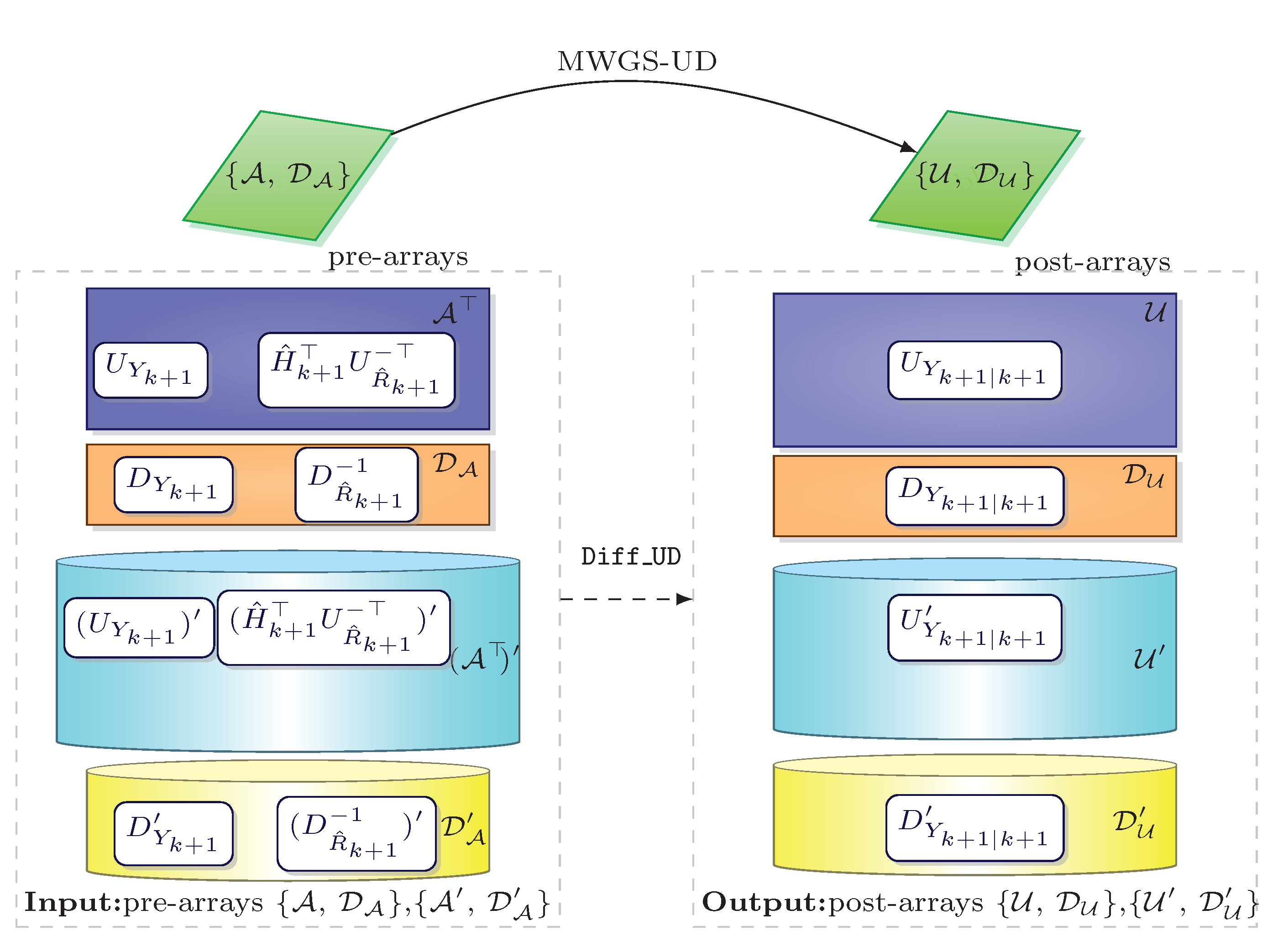
4.1. Implementation Details of Algorithm 4

Let us consider the computational scheme of the constructed algorithm in detail. The new Algorithm 4 is built based on one of two variants of the MWGS transformation and the corresponding method of algorithmic differentiation of such an orthogonal transformation. Therefore, Algorithms 2 and 3 can be considered as basic computational tools (or technologies) for the implementation of Algorithm 4. From this point of view, the technology of software implementation of the new algorithmic differentiation algorithm seems to be simple and understandable. It consists of only three simple steps:

• Fill in block pre-arrays with available data.
• Execute an algorithm for calculating derivatives in a matrix MWGS transformation of one of the types corresponding to Case 1 or Case 2.
• As a result, get block post-arrays and read off the required results from them in the form of matrix blocks.

The implementation scheme of the measurement update step in Algorithm 4 based on the MWGS-UD transformation is shown in Figure 1. Similarly, a general scheme for the MWGS-LD transformation can also be represented.

Figure 1. Implementation scheme of the measurement update step in Algorithm 4 based on the MWGS-UD transformation.

The computational complexity of the novel Algorithm 4 is mainly determined by the computational complexity of Algorithm 1, i.e., the MWGS-based information-form Kalman filtering algorithm. A detailed analysis of its computational complexity is given in ([18], Section 5.2).

It was shown that conventional IKF and Algorithm 1 have the complexity of the same order. However, IKF requires four full matrix inversions while calculating the information matrix Y. At the same time, Algorithm 1 requires only one full matrix inversion of the matrix $F_k$. Besides, if the matrices $Q_k$ and $R_k$ are positively definite and do not depend on k, then the modified Cholesky decomposition needs to be performed only once at the initialization step of the MWGS-based algorithm. If matrix $F_k$ is not singular and also does not depend on k, then the inversion of matrix F also needs to be performed only once, i.e., at the initialization step of the MWGS-based algorithm. Algorithm 4 requires additionally only one inversion of the unit triangular matrix and one inversion of the diagonal matrix (see Algorithm 2 or 3). Therefore, no additional inversions of the full matrices are required.

To summarize, the information matrix sensitivity evaluation based on the conventional IKF (Equations (5)–(7) and (19)–(23)) requires eight inversions of the full matrices, while the new Algorithm 4 avoids the full matrix inversion operations and requires the inverse of the unit triangular and diagonal matrices, only. Thus, we can conclude that the newly proposed algorithm is computationally efficient compared to the conventional IKF.

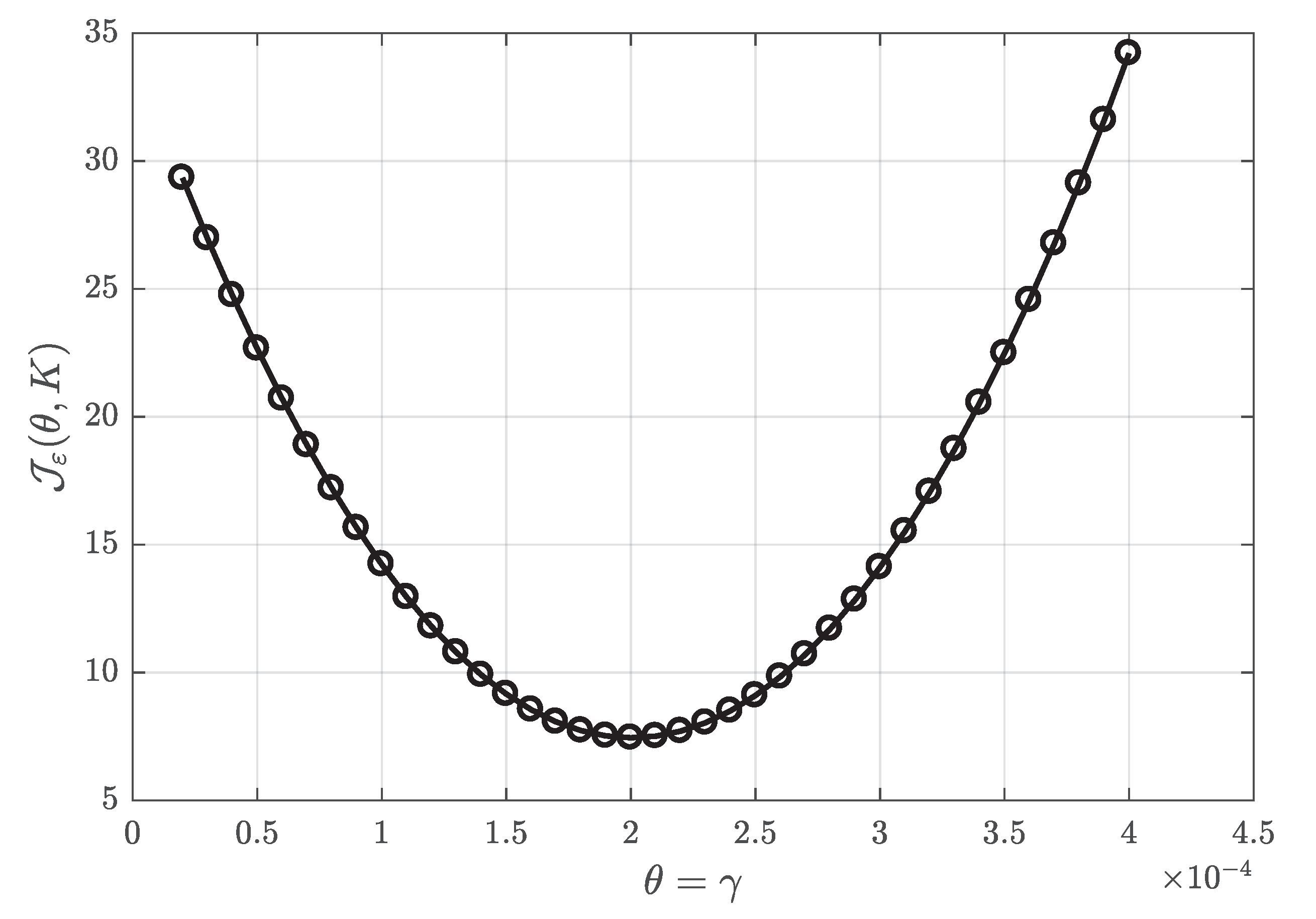
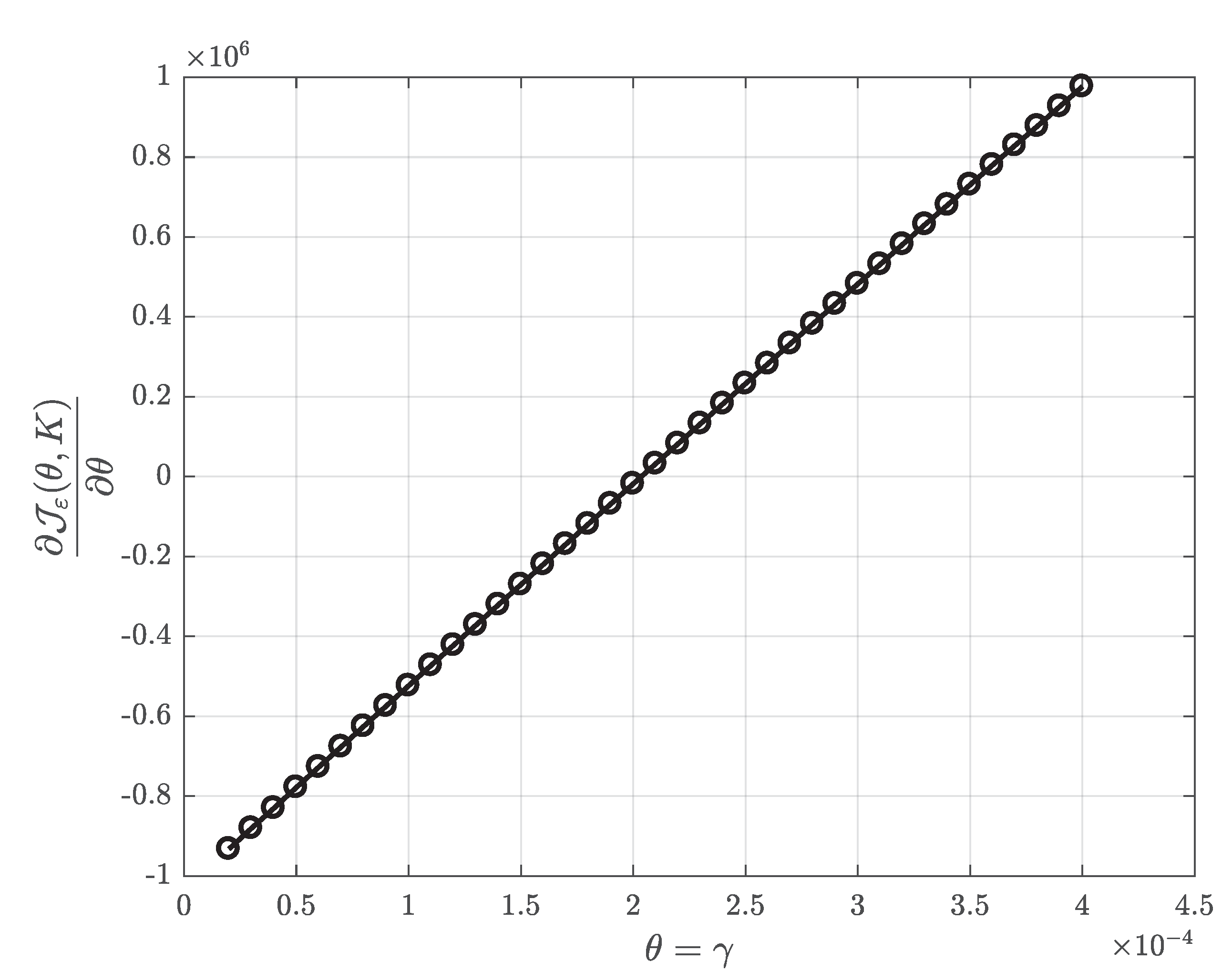
4.2. Application of the Results Obtained to the Problem of Parameter Identification

In practice, the matrices characterizing discrete-time linear stochastic system (1)–(2) are often known up to certain parameters. Consider an important problem of parameter identification [21]. Assume that the elements of system matrices $F_k\in {\mathbb{R}}^{n\times n}$, $G_k\in {\mathbb{R}}^{n\times q}$, $H_k\in {\mathbb{R}}^{m\times n}$, $Q_k\in {\mathbb{R}}^{q\times q}$, $R_k\in {\mathbb{R}}^{m\times m}$, and ${\Pi }_0\in {\mathbb{R}}^{n\times n}$ are functions of unknown system parameters vector $\theta \in {\mathbb{R}}^p$. It needs to be identified. For the sake of simplicity, instead of $F_k\left(\theta \right)$, $G_k\left(\theta \right)$, $H_k\left(\theta \right)$ etc., we will write $F_k$, $G_k$, $H_k$, etc.

We wish to demonstrate how the new Algorithm 4 can be applied to solve the parameter identification problem of the practical stochastic system model.

Consider the instrument error model for one channel of the INS (Inertial Navigation System) given as follows [25]:

$${\left[\begin{array}{c}\Delta v_x\\ \beta \\ m_{Ax}\\ n_{Gy}\end{array}\right]}_{k+1}=\left[\begin{array}{cccc}1& -\tau g& \tau & 0\\ \tau /a& 1& 0& \tau \\ 0& 0& b_1& 0\\ 0& 0& 0& 1\end{array}\right]{\left[\begin{array}{c}\Delta v_x\\ \beta \\ m_{Ax}\\ n_{Gy}\end{array}\right]}_k+\left[\begin{array}{c}0\\ 0\\ a_1\\ 0\end{array}\right]w_k,$$

(38)

$$z_{k+1}={(\Delta v_x)}_{k+1}+v_{k+1}$$

(39)

where $w_k\sim \mathcal{N}(0,1)$, $v_k\sim \mathcal{N}(0,0.01)$, $x_0\sim \mathcal{N}(0,I_4)$ and subscripts x, y, A, G denote “axis $Ox$”, “axis $Oy$”, “Accelerometer”, and “Gyro”, respectively.

The state vector $x_k={\left[\begin{array}{cccc}\Delta v_x,& \beta ,& m_{Ax},& n_{Gy}\end{array}\right]}^T$ where the first element is the random error in reading velocity along axis $Ox$ of a GSP, the second element is the angular error in determining the local vertical, the third one is the accelerometer reading random error, and the fourth one is the gyro constant drift rate.

The constants $\tau$, g, a are, respectively, equal to the rate of data arrival and processing, the gravity acceleration, and the semi-major axis of the Earth. The quantities $a_1=H_1\sqrt{1-b_1^2}\simeq H_1\sqrt{2\gamma \tau }$ and $b_1=e^{-\gamma \tau }\simeq 1-\gamma \tau$. The constants $H_1$ and $\gamma$ are elements of the accepted model of the correlation function $R_{m_{Ax}}=H_1^2{e}^{-\gamma \left|\tau \right|}$. Numerical values of the model parameters are given in Table 1.

Table 1. Numerical values of parameters.

Parameter	Value
$\tau$	$1\mathrm{s}$
g	$9.81\mathrm{m}/{\mathrm{s}}^2$
a	$0.6378245·{10}^7\mathrm{m}$
$b_1$	$e^{-\gamma \tau }\simeq 1-\gamma \tau$
$a_1$	$H_1\sqrt{1-b_1^2}\simeq H_1\sqrt{2\gamma \tau }$
$n_{Gy}$	$0.48·{10}^{-6}\mathrm{rad}/\mathrm{s}$
$H_1$	$0.10·{10}^{-3}\mathrm{m}/{\mathrm{s}}^2$
$\gamma$	$0.20·{10}^{-3}{\mathrm{s}}^{-1}$
$v_k$	$\sigma {\xi }_k$, ${\xi }_k\sim \mathcal{N}(0,1)$
$\sigma$	$0.1\mathrm{m}/\mathrm{s}$
$w_k$	$w_k\sim \mathcal{N}(0,1)$

Equations (38) and (39) correspond to the general model (1)–(2). Note that, in our case, all system model matrices do not depend on k.

Let us suppose that parameter $\gamma$ is unknown and needs to be identified. This means that the model parameter $\theta =\gamma$, and therefore $F=F\left(\theta \right)$, $G=G\left(\theta \right)$.

Solving the problem of parameter identification, we use the Active Principle of Adaptation (APA) [26,27,28,29], which consists of constructing an Auxiliary Performance Index (API) [23,28,30] and minimizing it with the use of a gradient-based numerical procedure.

The APA approach to system adaption within the parameter uncertainty differs in the fact that it suggests an indirect state prediction error control in the API form. It has to satisfy two main requirements:

• it depends on the system observable values only;
• it attains its minimum coincidently with the Original Performance Index (OPI).

The API satisfies a relation

$$\mathrm{API}=\mathrm{OPI}+const,$$

if the OPI is defined as the expected (Euclidean) norm of the state prediction error. Thus API and OPI have the one and the same minimizing argument ${\theta }^{†}$.

In order to construct the API, we build a Standard Observable Model (SOM), i.e., we perform the corresponding transformation of the basis in the state space from the representation (1)–(2). Model

$$\begin{array}{ccc}\hfill x_{k+1}^{*}& =& F_{*}\left(\theta \right)x_k^{*}+G_{*}\left(\theta \right)w_k,k\ge 0,\hfill \end{array}$$

(40)

$$\begin{array}{ccc}\hfill z_{k+1}& =& H_{*}{x}_{k+1}^{*}+v_{k+1}\hfill \end{array}$$

(41)

is equivalent to the original model (1)–(2) and is its canonical representation, where $x_k^{*}$ is the new state vector; $F_{*}\left(\theta \right)$, $G_{*}\left(\theta \right)$, and $H_{*}$ are matrices of the following form:

$$G_{*}=\tau a_1\left[\begin{array}{c}0\\ 1\\ 1+b_1\\ 1-\rho +b_1+b_1^2\end{array}\right],H_{*}=\left[\begin{array}{cccc}1& 0& 0& 0\end{array}\right],\rho ={\tau }^{2}g/a,$$

(42)

$$F_{*}=\left[\begin{array}{cccc}0& 1& 0& 0\\ 0& 0& 1& 0\\ 0& 0& 0& 1\\ -{\alpha }_4& -{\alpha }_3& -{\alpha }_2& -{\alpha }_1\end{array}\right],\begin{array}{c}{\alpha }_4=b_1(1+\rho ),\hfill \\ {\alpha }_3=-b_1(3+\rho )-(1+\rho ),\hfill \\ {\alpha }_2=3b_1+(3+\rho ),\hfill \\ {\alpha }_1=-b_1-3.\hfill \end{array}$$

(43)

From representation (42), (43) it follows that the maximum observability index of the system is $Ⓢ=4$.

Using the results of [26,27,28], we construct the auxiliary performance index (API)

$$J_{\epsilon }\left(\theta \right)\triangleq \frac{1}{2}\mathbb{E}\left\{{{\epsilon }_k\left(\theta \right)}^T{\epsilon }_k\left(\theta \right)\right\},$$

(44)

for which the auxiliary process is written in the form:

$${\epsilon }_k=\mathcal{S}\left(Z_{k+1-Ⓢ}^k\right)-{\widehat{x}}_{k+1-Ⓢ}={[z_{k-3},z_{k-2},z_{k-1},z_k]}^T-{\widehat{x}}_{k-3}$$

(45)

where ${\widehat{x}}_k$ is the prediction state estimate obtained in an adaptive filter.

Next, to get a reasonable estimate for (44), we replace it by the realizable (workable) performance index

$${\mathcal{J}}_{\epsilon }(\theta ,K)=\frac{1}{2K}\sum _{j=k-K+1}^k{{\epsilon }_j\left(\theta \right)}^T{\epsilon }_j\left(\theta \right).$$

(46)

With the purpose of finding the optimal value ${\theta }^{†}$ of the unknown parameter $\theta$ and to minimize the API (46), we can use existing methods of numerical optimization. Moreover, all non-search methods require the calculation of the API gradient. Assume that the gradient-based optimization method is chosen for the parameter identification procedure. Then, from (46), we can write the expression for calculating the API gradient:

$${\displaystyle \frac{\partial {\mathcal{J}}_{\epsilon }(\theta ,K)}{\partial \theta }=\frac{1}{K}\sum _{j=k-K+1}^k{\epsilon }_j^T\left(\theta \right)\frac{\partial {\epsilon }_j\left(\theta \right)}{\partial \theta }.}$$

(47)

Evaluating (47) requires the computation of sensitivities (partial derivatives) of the auxiliary process ${\epsilon }_j$ with respect to the adjustable parameter $\theta$. Various methods for calculating the sensitivities based on the standard Kalman filter are discussed in detail in [8].

Now, we are ready to demonstrate how the new Algorithm 4 can be applied for constructing a computational scheme for the numerical identification of the parameter $\theta$ based on the API approach.

Consider again the system model (42)–(43). Denote for simplicity $F=F_{*}\left(\theta \right)$, $G=G_{*}\left(\theta \right)$, $H=H_{*}$, ${\overline{x}}_0={\overline{x}}_0^{*}\left(\theta \right)$, ${\Pi }_0={\Pi }_0^{*}\left(\theta \right)$. Let $\theta =\gamma$, $Y_0={\Pi }_0^{-1}$, ${\widehat{d}}_{0|0}=Y_0{\overline{x}}_0$.

The identification of unknown parameter $\theta$ and the estimation of state vector $x_k$ of the system (38)–(39) according to the criterion

$${\theta }^{†}={\widehat{\theta }}_{\min }=\underset{\mathcal{D}\left(\theta \right)}{\mathrm{argmin}}{J}_{\epsilon }(\theta ,K)$$

(48)

can be performed simultaneously by the following algorithm.

Let us consider the practical application of Algorithm 5 to identify the unknown value of $\gamma$ in the model (38)–(39). We have simulated the sequence of output signals $Z_1^{200}$ with the “true” value of ${\gamma }^{†}=0.0002$. All computer codes were constructed in MATLAB.

In order to conduct our numerical experiments, we have implemented Algorithms 1–5 as the corresponding MATLAB functions. Then, we have calculated the API (46) and the API gradient (47) depending on different values of $\gamma$. Results are illustrated by Figure 2 and Figure 3.

Algorithm 5. The API-based parameter identification computational scheme.

BEGIN

✓ Assign an initial parameter estimate ${\widehat{\theta }}^i$ for $i=0$.    REPEAT 1° Take the current point ${\widehat{\theta }}^i$. 2° Evaluate the system matrices for (42)–(43) at ${\widehat{\theta }}^i$: $F_{*}:=F_{☆}\left({\widehat{\theta }}^i\right)$ , $G_{☆}:=G_{*}\left({\widehat{\theta }}^i\right)$. 3° Evaluate the matrix derivatives ${\left(F_{*}\right)}_{\theta }^{\prime }$ and ${\left(G_{*}\right)}_{\theta }^{\prime }$ at ${\widehat{\theta }}^i$. 4° Given the output data $Z_1^K={[z_1,\cdots ,z_K]}^T$, compute a value of the API at ${\widehat{\theta }}^i$ using (46) where the auxiliary process ${\epsilon }_j\left({\widehat{\theta }}^i\right)$ (45) can be evaluated as follows: $${\epsilon }_j\left({\widehat{\theta }}^i\right)=Z_{j-3}^j-{\widehat{x}}_{j-3}=Z_{j-3}^j-{Y_{j-3}}^{-1}{\widehat{d}}_{j-3}.$$ (49) The information matrix $Y_j=B_{Y_j}{D}_{Y_j}{B}_{Y_j}^T$ and information state estimate ${\widehat{d}}_j$ can be computed according to Algorithm 1 (the MWGS-based array IKF). 5° Evaluate the API gradient (47) at ${\theta }^i$ using the results of Step 3${}^{\circ }$ and the Algorithm 4. Wherein $${\displaystyle \frac{\partial {\epsilon }_j\left(\theta \right)}{\partial \theta }=-{\left({\displaystyle \frac{\partial Y_{j-3}}{\partial \theta }}\right)}^{-1}{\widehat{d}}_{j-3}-{\left(Y_{j-3}\right)}^{-1}\frac{\partial {\widehat{d}}_{j-3}}{\partial \theta },}$$ (50) ${\displaystyle \frac{\partial Y_j}{\partial \theta }=\frac{\partial \left(B_{Y_j}{D}_{Y_j}{B}_{Y_j}^T\right)}{\partial \theta }}$ are partial derivatives of information matrix $Y_j$. The partial derivative vector ${\displaystyle \frac{\partial {\widehat{d}}_j}{\partial \theta }}$ can be evaluated by direct differentiation of (16). 6° Find ${\theta }^{i+1}$ by the gradient-based optimization procedure $${\widehat{\theta }}^{i+1}={\widehat{\theta }}^i-{\beta }_i{\left.{\displaystyle \frac{\partial {\mathcal{J}}_{\epsilon }(\theta ,K)}{\partial \theta }}\right|}_{\theta ={\widehat{\theta }}^i}$$ (51) where scalar step size parameter ${\beta }_j$ is designed to ensure that ${\mathcal{J}}_{\epsilon }({\widehat{\theta }}^{i+1},K)\le {\mathcal{J}}_{\epsilon }({\widehat{\theta }}^i,K)+e$ (small $e>0$). 7° $i:=i+1$ UNTIL a stopping criterion is satisfied.

END

Figure 2. The values of the API identification criterion ${\mathcal{J}}_{\epsilon }(\theta ,K)$ depending on values of parameter $\theta$, calculated using Algorithms 1 and 5.

Figure 3. The values of the API gradient ${\displaystyle \frac{\partial {\mathcal{J}}_{\epsilon }(\theta ,K)}{\partial \theta }}$ depending on values of parameter $\theta$, calculated using Algorithms 4 and 5.

As can be seen from these figures, the minimum point of the API coincides with the true value of parameter $\theta ={\gamma }^{†}$. Furthermore, a plot of the API gradient has negative values to the left and positive values to the right of the zero point, which correspond to the minimum of the API. All this evidence substantiates our theoretical derivations.

Further to solve a parameter identification problem, we apply the MATLAB Optimization Toolbox with the built-in function fminunc, which implements the gradient-type method. Algorithm 5 was incorporated into the optimization method fminunc to compute the API and its gradient. We have chosen the initial value ${\widehat{\theta }}^0=0.001$ and the stopping criteria epsf=${10}^{-6}$, epsx=${10}^{-6}$.

Results summarized in Table 2 show that the computed estimate $\widehat{\theta }$ comes close to the true parameter value ${\gamma }^{†}$.

Table 2. Performance of the API-based identification of the model parameter $\gamma$.

“True” value ${\mathit{\gamma }}^{†}$	$0.0002$
Resulting estimate ${\widehat{\theta }}_{\min }$	$1.9999·{10}^{-4}$
${\mathcal{J}}_{\epsilon }({\widehat{\theta }}_{\min },K)$	$0.0196$
Relative estimation error $\left|\right|{\gamma }^{†}-{\widehat{\theta }}_{\min }\left|\right|/\left|\right|{\widehat{\theta }}_{\min }\left|\right|$	$7.8173·{10}^{-6}$

So, we conclude that the newly constructed Algorithm 4 can be efficiently applied to solve the parameter identification problem when the gradient-based optimization method is used.

5. Conclusions

This paper presents the new MWGS-based array algorithm for computing the information matrix sensitivity equations. We have extended the functionality of the MWGS-based information-form Kalman filtering methods so that they are able to calculate not only the values of the information matrix using the MWGS-based arrays, but also the values of their derivatives. The proposed algorithm is robust to machine round-off errors due to the application of the MWGS orthogonalization procedure at each step.

Moreover, we have demonstrated how the new Algorithm 4 can be applied for solving the parameter identification problem of the one practical stochastic system model, i.e., a simplified version of the instrument error model of the INS. We also have suggested the new API-based parameter identification computational scheme. Numerical experiments conducted in MATLAB confirm the efficiency of the proposed solution.

References

- Golub, G.H.; Van Loan, C.F. Matrix Computations; Johns Hopkins University Press: Baltimore, MD, USA, 1983. [Google Scholar]
- Giles, M. An Extended Collection of Matrix Derivative Results for Forward and Reverse Mode Algorithmic Differentiation; Report 08/01; Oxford University Computing Laboratory: Oxford, UK, 2008; 23p. [Google Scholar]
- Dieci, L.; Eirola, T. Applications of Smooth Orthogonal Factorizations of Matrices. In The IMA Volumes in Mathematics and Its Applications; Springer: New York, NY, USA, 2000; Volume 119, pp. 141–162. [Google Scholar]
- Dieci, L.; Russell, R.D.; Van Vleck, E.S. On the Computation of Lyapunov Exponents for Continuous Dynamical Systems. SIAM J. Numer. Anal. 1997, 34, 402–423. [Google Scholar] [CrossRef]
- Kunkel, P.; Mehrmann, V. Smooth factorizations of matrix valued functions and their derivatives. Numer. Math. 1991, 60, 115–131. [Google Scholar] [CrossRef]
- Dieci, L. On smooth decompositions of matrices. SIAM J. Matrix Anal. Appl. 1999, 20, 800–819. [Google Scholar] [CrossRef]
- Åström, K.-J. Maximum Likelihood and Prediction Error Methods. Automatica 1980, 16, 551–574. [Google Scholar] [CrossRef]
- Gupta, N.K.; Mehra, R.K. Computational aspects of maximum likelihood estimation and reduction in sensitivity function calculations. IEEE Trans. Autom. Control 1974, AC-19, 774–783. [Google Scholar] [CrossRef]
- Walter, S.F. Structured Higher-Order Algorithmic Differentiation in the Forward and Reverse Mode with Application in Optimum Experimental Design. Ph.D. Thesis, Humboldt-Universität zu Berlin, Berlin, Germany, 2011. [Google Scholar]
- Bierman, G.J. Factorization Methods for Discrete Sequential Estimation; Academic Press: New York, NY, USA, 1977. [Google Scholar]
- Grewal, M.S.; Andrews, A.P. Kalman Filtering: Theory and Practice Using MATLAB, 4th ed.; John Wiley & Sons, Inc.: New York, NY, USA, 2015. [Google Scholar]
- Kailath, T.; Sayed, A.H.; Hassibi, B. Linear Estimation; Prentice Hall: Hoboken, NJ, USA, 2000. [Google Scholar]
- Gibbs, B.P. Advanced Kalman Filtering, Least-Squares and Modeling: A Practical Handbook; John Wiley & Sons, Inc.: Hoboken, NJ, USA, 2011. [Google Scholar]
- Grewal, M.S.; Weill, L.R.; Andrews, A.P. Global Positioning Systems, Inertial Navigation, and Integration; John Wiley & Sons, Inc.: New York, NY, USA, 2001. [Google Scholar]
- Tsyganova, J.V.; Kulikova, M.V. State sensitivity evaluation within UD based array covariance filters. IEEE Trans. Autom. Control 2013, 58, 2944–2950. [Google Scholar] [CrossRef]
- Tsyganova, Y.V.; Tsyganov, A.V. On the Computation of Derivatives within LD Factorization of Parametrized Matrices. Bull. Irkutsk. State Univ. Ser. Math. 2018, 23, 64–79. (In Russian) [Google Scholar] [CrossRef]
- Kaminski, P.G.; Bryson, A.E.; Schmidt, S.F. Discrete square-root filtering: A survey of current techniques. IEEE Trans. Autom. Control 1971, AC-16, 727–735. [Google Scholar] [CrossRef]
- Tsyganova, J.V.; Kulikova, M.V.; Tsyganov, A.V. A general approach for designing the MWGS-based information-form Kalman filtering methods. Eur. J. Control 2020, 56, 86–97. [Google Scholar] [CrossRef]
- Björck, A. Solving linear least squares problems by Gram-Schmidt orthogonalization. Bit Numer. Math. 1967, 7, 1–21. [Google Scholar] [CrossRef]
- Tsyganova, J.V.; Kulikova, M.V.; Tsyganov, A.V. Some New Array Information Formulations of the UD-based Kalman Filter. In Proceedings of the 18th European Control Conference (ECC), Napoli, Italy, 25–28 June 2019; pp. 1872–1877. [Google Scholar]
- Ljung, L. System Identification: Theory for the User, 2nd ed.; Prentice Hall PTR: Upper Saddle River, NJ, USA, 1999. [Google Scholar]
- Kulikova, M.V. Likelihood Gradient Evaluation Using Square-Root Covariance Filters. IEEE Trans. Autom. Control 2009, 54, 646–651. [Google Scholar] [CrossRef]
- Semushin, I.V.; Tsyganova, J.V.; Tsyganov, A.V. Numerically Efficient LD-computations for the Auxiliary Performance Index Based Control Optimization under Uncertainties. IFAC-PapersOnline 2018, 51, 568–573. [Google Scholar] [CrossRef]
- Boiroux, D.; Juhl, R.; Madsen, H.; Jørgensen, J.B. An Efficient UD-Based Algorithm for the Computation of Maximum Likelihood Sensitivity of Continuous-Discrete Systems. In Proceedings of the 2016 IEEE 55th Conference on Decision and Control (CDC), ARIA Resort & Casino, Las Vegas, NV, USA, 12–14 December 2016; pp. 3048–3053. [Google Scholar]
- Broxmeyer, C. Inertial Navigation Systems; McGraw-Hill Book Company: Boston, MA, USA, 1956. [Google Scholar]
- Semushin, I.V. Adaptation in Stochastic Dynamic Systems—Survey and New Results I. Int. J. Commun. Netw. Syst. Sci. 2011, 4, 17–23. [Google Scholar] [CrossRef][Green Version]
- Semushin, I.V. Adaptation in Stochastic Dynamic Systems—Survey and new results II. Int. J. Commun. Netw. Syst. Sci. 2011, 4, 266–285. [Google Scholar] [CrossRef][Green Version]
- Semushin, I.V.; Tsyganova, J.V. Adaptation in Stochastic Dynamic Systems—Survey and New Results IV: Seeking Minimum of API in Parameters of Data. Int. J. Commun. Netw. Syst. Sci. 2013, 6, 513–518. [Google Scholar] [CrossRef]
- Semushin, I.V. The APA based time-variant system identification. In Proceedings of the 53rd IEEE Conference on Decision and Control (CDC), Los Angeles, CA, USA, 15–17 December 2014; pp. 4137–4141. [Google Scholar]
- Tsyganova, Y.V. Computing the gradient of the auxiliary quality functional in the parametric identification problem for stochastic systems. Autom. Remote Control 2011, 72, 1925–1940. [Google Scholar] [CrossRef]
Publisher’s Note: MDPI stays neutral with regard to jurisdictional claims in published maps and institutional affiliations. |
© 2022 by the authors. Licensee MDPI, Basel, Switzerland. This article is an open access article distributed under the terms and conditions of the Creative Commons Attribution (CC BY) license (https://creativecommons.org/licenses/by/4.0/).