An Algebraic Approach to Clustering and Classification with Support Vector Machines

Abstract

In this note, we propose a novel classification approach by introducing a new clustering method, which is used as an intermediate step to discover the structure of a data set. The proposed clustering algorithm uses similarities and the concept of a clique to obtain clusters, which can be used with different strategies for classification. This approach also reduces the size of the training data set. In this study, we apply support vector machines (SVMs) after obtaining clusters with the proposed clustering algorithm. The proposed clustering algorithm is applied with different strategies for applying SVMs. The results for several real data sets show that the performance is comparable with the standard SVM while reducing the size of the training data set and also the number of support vectors.

1. Introduction

In order to meet people’s demands, such as searching from the internet, taking high-quality pictures and videos, undergoing medical tests, widespread emails, producing multimedia contents, etc., there is a tremendous and continuous advancement in technology regarding data. Such interests require large digital storage with high-dimensional data sets. The data sets include both meaningful and irrelevant data, which is why ‘’data analysis” and ‘’data classification” topics are gaining more attention in recent years. Data analysis, providing predictions based on the training data, gave birth to machine learning.

Machine learning (ML) is a mega-trend in various fields and can be seen as a collection of computer algorithms that make life easier by predicting outcomes. Fundamentally, ML is based on algorithms (so-called “machines”) to automatically learn from observations (so-called “training data”) and to use the results for future decisions without explicit programming. ML algorithms have applications in almost all areas.

ML is generally categorized as either unsupervised learning (e.g., clustering), supervised learning (e.g., classification), or reinforcement learning (e.g., dynamic programming). In recent years, a new approach has been introduced: semi-supervised learning, which is a mixture of supervised learning and unsupervised learning. For semi-supervised learning, similarity-based approaches have also gained significant popularity in recent years (see, [1,2,3,4]).

In this paper, we propose a clustering algorithm that uses similarities between examples by associating weights to each attribute (according to their ability to separate classes) to reduce the size of the data set by combining the data as they form a so-called “clique”. The cliques have been heavily used in random matrix theory, and recently, this concept is being used in clustering algorithms (see, for example, [5,6,7]). More detail is given in Section 2.

Another important topic in ML is classification. Classification is a task for the predictive modeling problem. The aim of classification is to assign a class label for a given input data. There are several types of classification algorithms. Some well-known and widely used classification algorithms are Naive Bayes, Decision Trees, k-Nearest Neighbours, Logistic Regression, and Support Vector Machines.

Support vector machines (SVMs) are state-of-the-art classification methods used in various fields ([8,9,10]). There are many studies on extensions and improvements for SVMs. In some of these studies, SVMs are used with different clustering algorithms. For example, Wang et al., in [11], proposed KMSVM, which combines k-means clustering with SVMs. Chen et al., in [12], extend a least-squares twin support vector machine to a multiple-birth least-squares support vector machine for multi-class classification. Cheng et al., in [13], study local support vector machines for classification with nonlinear decision surfaces. Arslan et al. proposed a new clustering algorithm to discover the structure of the data set and then used these clusters with SVM in [2]. Another recent study [14] used the CURE clustering algorithm with SVMs. All these studies claim to obtain comparable performance with reduced training data set size and less support vectors. A brief introduction to SVMs is given in Section 3.

Motivated by these recent studies, we propose a new clustering algorithm based on cliques, named Clique Clustering Algorithm (CC-Algorithm). In Section 4, the CC-Algorithm is given. The algorithm is also demonstrated by an example in detail.

The main idea of using this clustering algorithm is to reduce the number of training data in the data set that will be used with SVMs (Section 5). There are three different algorithms proposed in this study: Centers of Cliques-SVM (CC-SVM), Homogeneous Cliques Removed-SVM (HOM-R-SVM), and Heterogeneous Cliques Removed-SVM (HET-R-SVM). Each proposed algorithm demonstrates different characteristics in terms of accuracy, performance, and data reduction ability.

2. Cliques and Clustering

As data sets become larger in size and complexity, data analysis has become the hit research topic in recent years. One of the main goals of clustering is to understand and analyze the data by splitting it into groups of similar items. Each group is named a cluster, and the method is focused on covering the data with a fewer number of clusters (details can be found from [15]). Although there is no significant definition for clusters since each method has clusters with its own shape, size, and density, it is extensively used in applications, such as web analysis [16], marketing [17], computational biology [18], data mining [19], machine learning [20], and many others.

Generating clusters is generally regarded as unsupervised learning because clustering does not use category labels, whereas classification is regarded as supervised learning. A new approach as a combination of unsupervised and supervised learning showed up in 2006 by Chapelle et al. [21], which is called semi-supervised learning. Most hybrid learning methods use various distance concepts for similarity functions. Similarity functions are generally defined by using Euclidean distance, Chebyshev distance, Jaccard distance, Mahalanobis distance, etc. Different distance functions result in different algorithms. For example, some graph-based approaches can be found in articles [4,22,23]. In [4], the data set represents a weighted graph that each data element is shown as a vertex and linking the vertices by the edges using a similarity value. However, Chen et al., in [22], proposed a partially observed unweighted graph. Ames et al. [6], on the other hand, considered the k-disjoint-clique optimization problem as a way to express the clustering problem with graphs and cliques. They claimed to solve this NP-hard optimization problem by using convex optimization.

A clique is a complete subgraph of an undirected graph, i.e., there is an edge between any pair of vertices. It was first used by Luce and Perry (1949) [24] in social networks and has many different applications in many areas other than graph theory.

In this study, we consider yet another approach for clustering, which is aimed at providing information from the data set that can be used with various classification strategies. We use cliques to obtain clusters. In our approach, the cliques and, therefore, the clusters are obtained with a heuristic algorithm. Instead of solving a problem like the densest k-disjoint-clique optimization problem, the proposed Algorithm 1 obtains dense cliques in a natural way by considering similarities between examples and by using a threshold value.

To achieve this, we subdivide the data into a number of disjoint cliques that maximize the sum of the weights of the edges inside of it. At first sight, the clique idea may look similar to the one in [6] where Euclidean distance is used for the weights of the edges. However, in this current study, the edge weight is calculated by using a similarity function that is totally different from the distance function. To the best of our knowledge, this is the first algorithm using cliques without using any distance function.

Definition 1.

The similarity value between two examples $x_i,x_j\in U$ with respect to an attribute $a\in A$, where A is the set of attributes and U is a finite set of objects, is defined as

$${\mathrm{sim}}_a(x_i,x_j)=1-\frac{|f(x_i,a)-f(x_j,a)|}{max\left(a\right)-min\left(a\right)}$$

for a numerical attribute $a,$ where ${\displaystyle max\left(a\right)=\underset{x_i\in U}{max}f(x_i,a),min\left(a\right)=\underset{x_i\in U}{min}f(x_i,a),}$ and $f(x,a)$ is a total function for each $a\in A$ and $x\in U$ and named the information function.

Remark 1.

$f(x_i,a)$ denotes the value of attribute a for the example $x_i$ of the data set $U.$

The similarity value defined above calculates the similarity between two vertices for a single attribute. In order to consider the total similarity with respect to a set of attributes, we use the similarity definition below, which is obtained by summing individual similarities using special weights.

Definition 2.

The similarity value between two examples $x_i,x_j\in U$ with respect to an attribute set $B\subseteq A$ is defined as

$$si{m}_B(x_i,x_j)=\sum _{a\in B}{w}_{a}si{m}_a(x_i,x_j)$$

(1)

where $w_a$ corresponds to the weight for an attribute $a\in B$.

As mentioned in the introduction, weights for attributes are calculated according to their performances for separating the classes. The detailed calculation of the weight for an attribute a is given as:

$$w_a=\frac{{\displaystyle \sum _{i=1}^{n}s\left(B_i\left(a\right)\right)}}{s\left(U\right)}$$

(2)

where $s\left(X\right)$ denotes the number of elements in the set $X,$ and $B_i$’s are defined as below:

$$\begin{array}{ccc}& & B_i\left(a\right)=A_i\left(a\right)\setminus \bigcup _{j=1(i\ne j)}^n{A}_j\left(a\right),\hfill \\ & & A_i\left(a\right)=\{x\in U|\min \left(C_i\left(a\right)\right)\le f(x,a)\le \max \left(C_i\left(a\right)\right)\},\hfill \end{array}$$

where $C_i\left(a\right)$ is the set of values for an attribute a belonging to class i, $1\le i\le n,$ and n is the number of classes in a data set. Equations (1) and (2) were introduced in [25], and we direct the reader to there for more details.

3. Support Vector Machines and Classification

Support vector machines (SVMs) were introduced by Vapnik and Chervenenkis in 1974 (see [26]). SVMs are one of the most popular methods used in ML (indeed, for supervised ML) with the aim of classifying given data by using so-called “training data”. For an introduction to the general theory of SVMs, we direct the reader to the sources [8,10,27,28,29] and to the papers [30,31,32,33] for recent developments, to name a few.

Basically, SVM is an algorithm for finding a separating hyperplane between two classes so that the margin between two classes is maximized. Suppose that the data set is given as $\left\{({\mathit{x}}_{\mathit{i}},y_i)\right|{\mathit{x}}_{\mathit{i}}\in {\mathit{R}}^n,y_i=\pm 1,\mathrm{for}i=1,2,\cdots ,\ell \}$, where $y_i$ denotes either of two possible classes $\{-1,1\},$ for simplicity. In order to find the optimal hyperplane whose normal vector is $\mathit{w}$ and given by Equation $\mathit{x}·\mathit{w}+b=0,$ one should consider the constraints:

$$\begin{array}{cc}\hfill {\mathit{x}}_{\mathit{i}}·\mathit{w}+b& \ge 1\mathrm{if}{y}_i=1,\hfill \\ \hfill {\mathit{x}}_{\mathit{i}}·\mathit{w}+b& \le -1\mathrm{if}{y}_i=-1,\hfill \end{array}$$

which can be combined together as

$$y_i({\mathit{x}}_{\mathit{i}}·\mathit{w}+b)-1\ge 0\mathrm{for}i=1,2,\cdots ,\ell .$$

By requiring (if necessary, after rescaling $\mathit{w}$ and b) that there are some points satisfying the two inequalities as an equality (such points are called “support vectors”), the margin between two classes turns out to be $2/\left|\right|\mathit{w}\left|\right|.$ Hence, in order to find the hyperplane providing the maximum margin between two classes, it is enough to minimize $\left|\right|\mathit{w}\left|\right|$ or equivalently and more simply ${\left|\right|\mathit{w}\left|\right|}^2.$ By using Lagrange multipliers, ${\lambda }_i$ for $i=1,\cdots ,\ell ,$ one obtains the Lagrangian

$$F(\mathit{w},b,{\lambda }_1,\cdots ,{\lambda }_{\ell })=\frac{1}{2}{\left|\right|\mathit{w}\left|\right|}^2-\sum _{i=1}^{\ell }{\lambda }_i{y}_i({\mathit{x}}_{\mathit{i}}·\mathit{w}+b)+\sum _{i=1}^{\ell }{\lambda }_i.$$

We direct the reader to [8] for a comprehensive and complete account of the remaining convex optimization.

If there is no feasible solution to this optimization problem, i.e., when the data are not separable by a hyperplane, then by introducing extra positive slack variables, ${\xi }_i,$ representing the error (when ${\xi }_i>1$), the above constraints can be rewritten as:

$$\begin{array}{cc}\hfill {\mathit{x}}_{\mathit{i}}·\mathit{w}+b& \ge 1-{\xi }_i\mathrm{if}{y}_i=1,\hfill \\ \hfill {\mathit{x}}_{\mathit{i}}·\mathit{w}+b& \le -1+{\xi }_i\mathrm{if}{y}_i=-1,\hfill \\ \hfill {\xi }_i& \ge 0.\hfill \end{array}$$

In this case, the objective function to be minimized is also changed from

$$\frac{{\left|\right|\mathit{w}\left|\right|}^2}{2}$$

to

$$\frac{{\left|\right|\mathit{w}\left|\right|}^2}{2}+C\sum _{i=1}^{\ell }{\xi }_i,$$

where C is a cost parameter for the sum of error terms.

For data sets where classes are non-linearly separated (i.e., when they are separated by some hypersurface), one can use the kernel trick and transform the data set into a higher dimensional Euclidean space by using an appropriate kernel function $K({\mathit{x}}_{\mathit{i}},{\mathit{x}}_{\mathit{j}})$. The most common used kernel functions for real-life data in pattern recognition are listed in

Table 1. Common kernel functions.

Kernel Name	Kernel Function
Linear ($k=1$):	$K({\mathit{x}}_{\mathit{i}},{\mathit{x}}_{\mathit{j}})={\mathit{x}}_{\mathit{i}}·{\mathit{x}}_{\mathit{j}}$
Gaussian Radial Basis ($k=2$):	$K({\mathit{x}}_{\mathit{i}},{\mathit{x}}_{\mathit{j}})=e^{-\left|\right|{\mathit{x}}_{\mathit{i}}-{\mathit{x}}_{\mathit{j}}{\left|\right|}^2/2{\sigma }^2}$
Polynomial ($k=3$):	$K({\mathit{x}}_{\mathit{i}},{\mathit{x}}_{\mathit{j}})={(\gamma {\mathit{x}}_{\mathit{i}}·{\mathit{x}}_{\mathit{j}}+\delta )}^p$
Sigmoid ($k=4$):	$K({\mathit{x}}_{\mathit{i}},{\mathit{x}}_{\mathit{j}})=tanh(\gamma {\mathit{x}}_{\mathit{i}}·{\mathit{x}}_{\mathit{j}}+\delta )$

(see [34] for details):

In this study, all kernel functions above are tested for each data set, and the best fitted results are chosen with respect to the Standard SVM without reducing any of the data, as will be later explained in Section 5. Among the 10 data sets used in this study, the best performance is obtained with a linear kernel for 3 of them and with a radial basis kernel for 7 of them. The details are summarized in the Table 3.

4. A Clique Clustering Algorithm

In this section, the “Clique Clustering Algorithm” (CC-Algorithm) is introduced in Algorithm 1, and a detailed example is given for demonstrating the steps of the algorithm. We note here that the proposed CC-Algorithm starts with the most similar pair of examples to construct the cliques. Thus, the cliques obtained naturally represent highly dense cliques.

Notation 1.

The following notations and assumptions are being used in the algorithm below, with some conventions to simplify the algorithm and its implementation. Let C denote the set of all attributes for the given data set.

B is a list of index pairs ordered in the decreasing order with respect to the similarity function $si{m}_C(x_i,x_j),$ such that, for $k<\ell ,$

$$\begin{array}{cc}\hfill \mathit{either},& si{m}_C(x_{k_1},x_{k_2})>si{m}_C(x_{{\ell }_1},x_{{\ell }_2}),\hfill \\ \hfill \mathit{or},& si{m}_C(x_{k_1},x_{k_2})=si{m}_C(x_{{\ell }_1},x_{{\ell }_2}),\mathit{and}{k}_1>l_1\hfill \\ \hfill \mathit{or},& si{m}_C(x_{k_1},x_{k_2})=si{m}_C(x_{{\ell }_1},x_{{\ell }_2}),k_1=l_1,\mathit{and}{l}_2>k_2\hfill \end{array}$$

where $B\left[k\right]=(k_1,k_2)\mathit{and}B[\ell ]=(l_1,l_2)$, and $B\left[m\right]$ denotes the m-th element of the ordered list, $B.$ Hence, for example, $B\left[1\right]$ denotes the index $(i,j)$, where $si{m}_C(x_i,x_j)$ is the largest. The same ordering is also used for sorting the list A in Step 2.(c) of the algorithm.

Moreover, to avoid repetitions, we assume without loss of generality that $i<j$ for any $(i,j)\in B.$ Furthermore, empty list is denoted by $\left[\right].$

The clique clustering algorithm is presented below. Algorithm 1.

Algorithm 1: Clique Clustering (CC) Algorithm.

Input:$B,t,si{m}_C(x_i,x_j).$ Output: List of Cliques, $L.$ Let B denote the ordered list set of all pairs $(i,j)$ with $sim(x_i,x_j)\ge t$ for a given threshold t, and this list is ordered by the similarity values from largest to smallest. Set $L:=\left[\right]$ and $B_0:=B.$ Repeat until $B_0=\left[\right]$ ∖# The below sub-algorithm will repeat until all pairs in the list B have been considered. #∖ (a) Let $(i,j)=B_0\left[1\right]$ be the first element. $\setminus$# I.e., the pair $(i,j)$ such that $sim(x_i,x_j)$ is the largest value. #∖ (b) Consider the index sets $A_i=\left\{k\right|(i,k)\in B_0\mathrm{or}(k,i)\in B_0\}$ and $A_j$ similarly, and then form a list from intersection of $A_i$ and $A_j$; $A=[k:k\in A_i\cap A_j].$ ∖# $A_i$ is the index set of vertices $x_k$ where there is an edge between $x_i$ and $x_k$; similarly, $A_j$ is the index set of vertices $x_k$ where there is an edge between $x_j$ and $x_k,$, and hence, A is the list of indices k such that $\{x_i,x_j,x_k\}$ forms a clique. #∖ (c) Sort A as an ordered list by similarity values from largest to smallest according to $sim(x_i,x_k)$ for $i<j$ and $k\in A.$ ∖# In order to obtain the densest cliques, we will check each element of A one by one, after checking whether the remaining elements are included in the clique or not. #∖ (d) Set $A_0:=A$ Repeat until $A_0=\left[\right]$ ∖# The below sub-routine will repeat until all indices in the list $A_0$ have been considered. #∖ Let $k=A_0\left[1\right]$ be the first element. ∖# Densest clique construction: As conducted before, $k\in A_0$ with largest similarity value of $sim(x_i,x_k).$ #∖ $A_0:=\mathrm{Remove}(A_0,\left[k\right]).$ $A_k:=\{\ell \in A|(k,\ell )\in B_0\mathrm{or}(\ell ,k)\in B_0\}.$ ∖# Find all vertices $x_{\ell },\ell \in A_0,$ such that $sim(x_k,x_{\ell })\ge t.$ Recall that $B_0$ is the set of index pairs $(k,\ell )$ for which $sim(x_k,x_{\ell })\ge t.$ Hence, either $(k,\ell )\in B_0$ or $(\ell ,k)\in B_0.$ #∖ Find, if any, vertices $x_{\ell }$ such that there is no edge between $x_k$ and $x_{\ell }.$ $D:=[\ell :\ell \in A\wedge \ell \notin A_k]$ ∖# If there exists such $\ell \in D,$ any set of vertices containing $\{x_k,x_{\ell }\}$ cannot form a clique. Thus, we should remove such elements from A for the clique under construction. #∖ Update A and $A_0$ as $A:=\mathrm{Remove}(A,D)$ and $A_0:=\mathrm{Remove}(A_0,D).$ ∖# The set A is reduced by removing some elements. In order to check the remaining elements for forming a clique, we also remove them from the iteration set $A_0$ and repeat with the next element. #∖ Next ∖# until $A_0=\left[\right]$ #∖. (e) $L:=\mathrm{Append}(L,[A\left]\right)$ update the list $L.$ ∖# A clique is obtained, $A,$ and added to the list of cliques. Now, we will remove from $B_0$ any pair associated with clique vertices. #∖ (f) For each $k\in A,$ set $R_k=\left\{(k,\ell )\right|(k,\ell )\in B_0\}\cup \left\{(\ell ,k)\right|(\ell ,k)\in B_0\}.$ (g) $R={\cup }_{k\in A}{R}_k.$ (h) $B_0:=\mathrm{Remove}(B_0,[\ell :\ell \in R]).$ (i) Next ∖# until $B_0=\left[\right]$ #∖. Return $L.$

An Example

The following sample data were obtained from the Iris data set, selecting 60 rows, 20 from each class, randomly. Moreover, in order to demonstrate the clique algorithm above, only the first two attributes were used, see Figure 1.

For chosen attributes, $a_1,a_2,$ the weights of each attribute are calculated from the sample and represented as a vector $w=(0.7419,0.2581)$, as described in Section 2. Then, according to this weight vector, the similarities are calculated:

Seq.	Sim.	i	j
$\left[1\right]$	1.0000	38	52
$\left[2\right]$	1.0000	36	56
$\left[3\right]$	1.0000	33	58
	⋮
$\left[1768\right]$	0.2065	14	48
$\left[1769\right]$	0.1865	14	44
$\left[1770\right]$	0.1865	14	45

After choosing a threshold, in this example, $t=0.90,$ we obtain only the first 255 rows from the above table:

Seq.	Sim.	i	j
	⋮
$\left[253\right]$	0.9001	29	39
$\left[254\right]$	0.9001	27	30
$\left[255\right]$	0.9001	8	23

Performing the CC-Algorithm described above, we obtain the cliques;

Clq.	$i_1$	$i_2$	$i_3$	$i_4$	$i_5$	$i_6$	$i_7$	$i_8$
$\left[1\right]$	38	52	30	34	51	60
$\left[2\right]$	36	56	25	28	35	39	40	43
$\left[3\right]$	33	58	22	26	32	55	57	59
⋮	⋮
$\left[10\right]$	23	41
$\left[11\right]$	42	50
$\left[12\right]$	3	12

Among 60 examples, 55 are listed in the first 255 rows above. With the clique algorithm, these 55 example are separated into 12 disjoint subsets. Among 12 cliques, 7 of them are homogeneous, i.e., all examples belonging to a clique have the same class type. The remaining five cliques are heterogeneous, all having examples exactly from two different classes. In Figure 2, all 12 cliques are shown with different colors, and the remaining 5 data (55 out of 60 are already in cliques) are marked as Clique 0 for completeness and simplicity.

5. The Proposed Classification Algorithms

The idea of using clustering as an intermediate step before applying learning algorithms is an active research topic. For example, [11] proposed KMSVM, which combines k-means clustering with SVMs. In [14], a well-known clustering algorithm (CURE) is applied to discover the structure of the training data set before applying SVMs. In this study, we propose yet another approach by using the proposed CC-Algorithm. Different from the previous studies in the literature, the proposed approach uses the concept of complete cliques to obtain clusters of the training data set.

The main idea of the proposed classification algorithms is to discover structural information of the data by using the proposed clique clustering approach. We expect that this will reduce the training data set size while at the same time improving the classification algorithm.

Although one may consider different strategies to achieve this goal, in this study, we considered three basic strategies. In the first strategy, the centers of the cliques are used for training the SVM. This algorithm will be called the Centers of Cliques-SVM (CC-SVM). In the second strategy, cliques contain only one class category, i.e., homogeneous cliques are removed and heterogeneous cliques are replaced with their centers before applying SVM. This approach will be called the Homogeneous Cliques Removed-SVM (HOM-R-SVM). In the third strategy, cliques contain more than one class category, i.e., heterogeneous cliques are removed and homogeneous cliques are replaced with their centers before applying SVM. This approach will be called the Heterogeneous Cliques Removed-SVM (HET-R-SVM).

All three approaches will reduce the original training data set size by some amount. This will also affect the selection of support vectors. It is expected that this will result in avoiding some of the over-fitting problems that may be encountered.

After applying the clique-clustering algorithm, the training set will be partitioned into two parts: the cliques denoted by $\mathcal{C}$ and the remaining elements denoted by $\mathcal{F}$. Assuming that there are l cliques and r remaining elements, we have $\mathcal{C}=\left\{{\mathcal{C}}_1,{\mathcal{C}}_2,\dots ,{\mathcal{C}}_l\right\}$ and $\mathcal{F}=\left\{{\mathit{x}}_1,{\mathit{x}}_2,\dots ,{\mathit{x}}_r\right\}$, where ${\mathit{x}}_j\in {\mathit{R}}^d$.

5.1. Centers of Cliques (CC-SVM) Algorithm

The basic idea in this approach is to use the cliques to reduce the data set by replacing each clique with its center. The main steps of this approach are as follows:

• Apply the Clique Clustering Algorithm (CC-Algorithm in Section 4).
• Find centers for each class category in each clique.

  (a)

  For homogeneous cliques, only one center is calculated.

  (b)

  For heterogeneous cliques, we further identify all classes appearing in the clique and calculate the centers of data having the same class label. Thus, we obtain a minimum of two centers for each clique.

  (c)

  Elements in $\mathcal{F}$ are also considered centers of cliques of size one.

• Apply the SVM algorithm.

If we analyze our previous sample example, the number of examples is reduced to $5+7+2\times 5=22$ data, corresponding to 5 data from $\mathcal{F};$ 7 data from homogeneous cliques, each clique is replaced with its center; and 10 data, 2 from each of the 5 heterogeneous cliques containing examples from two classes and within each such clique, and centers are calculated for each group of data that has the same class labels. All details are illustrated in Figure 3, where all orange arrows show a reduction within homogeneous cliques belonging to “setosa” class, and most green and blue arrows show a reduction within heterogeneous cliques; however, there is one homogeneous green clique and there are two homogeneous blue cliques. With 22 data, we obtain a better accuracy level when compared with the standard SVM using all 60 data.

5.2. Homogeneous Cliques Removed (HOM-R-SVM) Algorithm

The basic idea of this approach is to reduce the data set by removing homogeneous cliques and replacing each heterogeneous clique with their centers. The main steps of this approach are as follows:

• Apply the CC-Algorithm.
• Remove cliques that contain only one class category.

  (a)

  Remove all data in homogeneous cliques.

  (b)

  For heterogeneous cliques, replace heterogeneous cliques with their centers. As in CC-SVM, calculate the centers of the data that have the same class labels.

  (c)

  The elements in $\mathcal{F}$ are also considered as the training data set.

• Apply SVM algorithm.

For our sample example, the number of examples is reduced to $5+2\times 5=15$ data only. All details are illustrated in Figure 4. Then, the standard SVM is applied only to these 15 data. The resulting accuracy level is comparable to the accuracy of the standard SVM with fewer examples.

5.3. Heterogeneous Cliques Removed (HET-R-SVM) Algorithm

The basic idea of this approach is to reduce the data set by removing heterogeneous cliques and replacing each homogeneous clique with its center. The main steps of this approach are as follows:

• Apply the CC-Algorithm.
• Remove cliques that contain more than one class categories.

  (a)

  For homogeneous cliques, replace any clique with its center.

  (b)

  For heterogeneous cliques, remove all data lying inside a clique that has more than one class category.

  (c)

  Elements in $\mathcal{F}$ are also considered as centers of cliques of size one.

• Apply SVM algorithm.

Finally, for the sample example, the number of examples is reduced to $5+7=12$ data. All details are illustrated in Figure 5. The result is the same as the standard SVM with fewer examples.

6. Application to Real Data Sets and Performance

In order to analyze the performance of the proposed classifiers, we considered 10 data sets that have also been used in some other studies (see, for example, [2,14,25]). We note that all data sets have numerical attributes only. The data sets represent different application areas and various properties. Some of them have a relatively large number of class categories, whereas some have a relatively large number of examples, see

Table 2. Summary of Data Sets.

Data Set	n	a	c	Area
Iris	150	4	3	Life
Wine	178	13	3	Physical
Glass	214	9	7	Physical
Connectionist Bench	208	60	2	Physical
(Sonar_All)
Statlog (Vehicle)	846	18	4	Physical
Ionosphere	351	33	2	Physical
Blood Transfusion	748	4	2	Business
Ecoli	336	6	8	Life
Haberman’s Survival	306	3	2	Life
Breast Cancer Wisconsin	683	9	2	Life

.

A few of the data sets needed some slight changes or adjustment before applying the algorithms. For example, 16 rows from “Breast Cancer Wisconsin” have missing values in one attribute, so for consistency, all these 16 rows have been deleted. For the “Ionosphere” data set, the second attribute is constant for all instances, so this attribute is completely removed before using the data. For the “Ecoli” data set, the fourth attribute (presence of charge) is almost constant, and all the columns are equal to 0.5, except for one row with a value of 1. Since train and test data are randomly chosen, for the cases where the data with the exceptional value of 1 for this attribute belong to test data, the SVM will report an error. For this reason, the fourth attribute is completely removed from this data set before running simulations.

Figure 6 shows the performance of all three proposed algorithms in terms of accuracy. In general, it is clear from the figure that the proposed classification algorithms achieve similar accuracy results as for the standard SVM with a reduced training data set size and fewer support vectors. For the Ecoli, Glass, and Blood Transfusion data sets a decrease in accuracy is observed. The degree of decrease depends on the particular algorithm. For example, for the Ecoli and Glass data sets, there is quite a decrease in accuracy for the HET-R-SVM algorithm. On the other hand, for the Blood Transfusion data set, the worst performance is obtained with the HOM-R-SVM algorithm. Finally, one can also see that the CC-SVM algorithm shows a more robust behavior compared to the other proposed SVM algorithms.

Instead of comparing the accuracy values of the test data for each data set, we provide detailed analysis of the results in

Table 3. The summary of SVM algorithms’ simulations.

Data Set	k	t	Std. SVM				HOM-R-SVM				HET-R-SVM				CC-SVM
			n	${\mathit{n}}_{\mathit{s}}$	Acc.		${\mathit{n}}_{\mathit{t}}$	${\mathit{n}}_{\mathit{s}}$	Acc.		${\mathit{n}}_{\mathit{t}}$	${\mathit{n}}_{\mathit{s}}$	Acc.		${\mathit{n}}_{\mathit{t}}$	${\mathit{n}}_{\mathit{s}}$	Acc.
Iris	1	0.95	105	22.8	0.956		20	12.6	0.947		38	14	0.956		41.2	16.6	0.956
Wine	2	0.95	125	61.8	0.985		112.6	59.2	0.985		118.8	60.4	0.985		118.8	60.4	0.985
Glass	2	0.95	150	132	0.681		39	38.8	0.509		23.4	22.2	0.391		46	44.6	0.525
Sonar_All	2	0.95	146	117	0.829		135.2	111.6	0.826		140.2	114.2	0.832		140.2	114.2	0.832
Vehicle	1	0.95	592	322	0.808		314.8	218.8	0.749		248.6	147.2	0.785		401.6	252.8	0.787
Ionosphere	2	0.95	246	100	0.933		132.2	82.8	0.916		158	83.6	0.935		162	88	0.935
Transfusion	2	0.85	524	266.8	0.777		15.6	15.6	0.662		3.2	2.4	0.462		17.6	17.2	0.671
		0.95					63.2	59.8	0.621		22.6	16.2	0.719		74.6	65.4	0.661
Ecoli	1	0.90	235	94.4	0.822		15.2	14.4	0.766		4.8	4.0	0.410		15.6	14.4	0.760
Haberman’s Survival	2	0.95	214	121.8	0.748		75.8	71.2	0.609		41.4	31.8	0.752		90.6	81.2	0.759
Breast Cancer Wisconsin	2	0.95	478	74.2	0.966		189.8	63.2	0.967		216.4	62.4	0.967		216.8	63.2	0.967

. In this table, k denotes the kernel as given in Table 1, t denotes the threshold used in the clique algorithm in Section 4, n denotes the number of the training data set for “Std. SVM” and the average number of reduced data of the corresponding SVM for five runs, whereas $n_s$ similarly denotes the number of support vectors for each SVM, and finally, “Acc.” denotes the accuracy of the classification of the test data obtained for each SVM.

The results in Table 3 show that, overall, the proposed algorithms achieve the same accuracy with a smaller training data set size and fewer support vectors. Only for the Wine and Sonar_All data sets, the reduction may be negligible, but this is indeed to achieve the best performance. For example, for the Wine data set, instead of $t=0.95,$ if $t=0.90$ is considered, then $n_t=30.6,n_s=28,\mathrm{Acc}.=0.868$ for HOM-R-SVM; and $n_t=59.4,n_s=39.6,\mathrm{Acc}.=0.981$ for HET-R-SVM; and $n_t=61,n_s=41.2,\mathrm{Acc}.=0.981$ for CC-SVM. Similarly, for Sonar_All data set, instead of $t=0.95,$ if $t=0.85$ is considered, then $n_t=58.6,n_s=57.4,\mathrm{Acc}.=0.761$ for HOM-R-SVM; and $n_t=59.2,n_s=55.2,\mathrm{Acc}.=0.797$ for HET-R-SVM; and $n_t=77.2,n_s=73,\mathrm{Acc}.=0.816$ for CC-SVM.

For the Transfusion data set, we decided to report two different threshold values, $t=0.85$ and $t=0.95$, because, for the former one, HOM-R-SVM and CC-SVM have better accuracy values for the test data; however, for the later one, HET-R-SVM performs much better.

In addition to the accuracy rates given in Table 3,

Table 4. TP rates, FP rates and AUC analysis.

Data Set	k	t	Std. SVM				HOM-R-SVM				HET-R-SVM				CC-SVM
			TP Rate	FP Rate	ROC Area		TP Rate	FP Rate	ROC Area		TP Rate	FP Rate	ROC Area		TP Rate	FP Rate	ROC Area
Iris	1	0.95	0.978	0.009	0.984		0.956	0.018	0.969		0.956	0.018	0.969		0.978	0.009	0.984
Wine	2	0.95	0.981	0.011	0.985		0.981	0.011	0.985		0.981	0.011	0.985		0.981	0.011	0.985
Glass	2	0.95	0.625	0.143	0.741		0.516	0.127	0.694		0.422	0.219	0.601		0.531	0.141	0.695
Sonar_All	2	0.95	0.629	0.450	0.589		0.548	0.548	0.500		0.597	0.490	0.554		0.597	0.49	0.554
Vehicle	1	0.95	0.780	0.074	0.853		0.720	0.094	0.813		0.728	0.091	0.819		0.756	0.082	0.837
Ionosphere	2	0.95	0.924	0.146	0.889		0.914	0.098	0.908		0.924	0.146	0.889		0.924	0.146	0.889
Transfusion	1	0.95	0.790	0.754	0.518		0.714	0.472	0.621		0.692	0.539	0.577		0.580	0.372	0.604
Ecoli	1	0.94	0.788	0.072	0.858		0.768	0.054	0.855		0.712	0.154	0.735		0.663	0.082	0.790
Haberman’s Survival	2	0.95	0.739	0.699	0.520		0.641	0.660	0.490		0.728	0.728	0.500		0.707	0.661	0.523
Breast Cancer Wisconsin	2	0.95	0.946	0.026	0.960		0.937	0.031	0.953		0.937	0.031	0.953		0.937	0.031	0.953

shows the true positive (TP) rate, false positive (FP) rate, and ROC areas for the data sets considered in this study. These results were calculated using the WEKA software [35] after obtaining the clique clusters with the proposed clustering algorithm. The results confirm the analysis given for Table 3. In general, almost the same performance as the standard SVM is obtained with the proposed algorithms using reduced training data sets in terms of TP and FP rates as well as ROC area.

The reduction in training size and number of support vectors is very high for most of the data sets. In addition, one can observe that the CC-SVM algorithm achieves comparable (sometimes even better) accuracy for all data sets compared to the standard SVM. On the other hand, HOM-R-SVM achieves the best results for the Iris and Breast Cancer Wisconsin data sets, whereas HET-R-SVM achieves the best results for the Vehicle and Haberman’s Survival data sets. Details about the amount of reduction is given in Figure 7, Figure 8 and Figure 9 for each algorithm separately for the data ratio versus accuracy ratio. In these charts, the following ratios are represented:

$$\mathrm{Data}\mathrm{ratio}=\frac{n_t\mathrm{for}\mathrm{the}\mathrm{proposed}\mathrm{SVM}}{n\mathrm{for}\mathrm{the}\mathrm{standard}\mathrm{SVM}},$$

and

$$\mathrm{Accuracy}\mathrm{ratio}=\frac{\mathrm{Accuracy}\mathrm{of}\mathrm{test}\mathrm{data}\mathrm{for}\mathrm{the}\mathrm{proposed}\mathrm{SVM}}{\mathrm{Accuracy}\mathrm{of}\mathrm{test}\mathrm{data}\mathrm{for}\mathrm{the}\mathrm{standard}\mathrm{SVM}}.$$

Figure 7 shows that, overall, CC-SVM achieves almost the same performance as the standard SVM with a reduced training data set. Only for the Glass data set a significant decrease in accuracy is observed, which is still the best among the three proposed algorithms. In addition, for the Ecoli, Iris, and Blood Transfusion data sets, the data reduction is very high with ratios of less than 8%.

Figure 8 shows that overall HOM-R-SVM achieves comparable performance to the standard SVM with a reduced training data set. Only for the Glass data set a significant decrease in accuracy is observed. In addition, for the Ecoli and Transfusion data sets, the data reduction is very high with ratios of less than 7%.

Figure 9 shows that, overall, HET-R-SVM achieves almost the same performance as the standard SVM with a reduced training data set, except for the Ecoli and Glass data sets. For these two data sets, a significant decrease in accuracy is observed. In addition, for the Ecoli, Haberman, and Transfusion data sets, the data reduction is very high with ratios of less than 6%.

These results also show that all three algorithms actually capture some different aspects of the data sets. For example, although the best performance (with an accuracy ratio of 1.02 and data reduction ratio of 0.42) for the Haberman data set is obtained with the CC-SVM algorithm, the HET-R-SVM shows a similar performance (with an accuracy ratio of 0.97) with only a fraction of 6% of the original training data set.

7. Discussion

The results show that for most of the data sets, the three algorithms show similar performances. For example, for the BC-Wisconsin and Wine data sets, all three algorithm show a similar performance and data reduction behavior. In contrast, for the Ecoli, Glass, and Transfusion data sets, the algorithms show some clear differences. For example, for the Ecoli data set, only the HET-R-SVM shows a significant decrease in accuracy compared to the standard SVM. For the Glass data set, all three algorithms achieve less accuracy compared to the standard SVM. For this data set, the best accuracy is achieved with the CC-SVM algorithm. For the Transfusion data set, the best accuracy is achieved with the HET-R-SVM algorithm.

In summary, one can see that for some data sets, all three algorithms show similar performances. Conversely, for some data sets, one of the algorithms shows the best performance. Thus, for some of the data sets, as expected, either HOM-R-SVM or HET-R-SVM may perform better than the usual scenario where CC-SVM performs better. The choice of the corresponding algorithms depends on the user’s needs and the structure of the data set or classes.

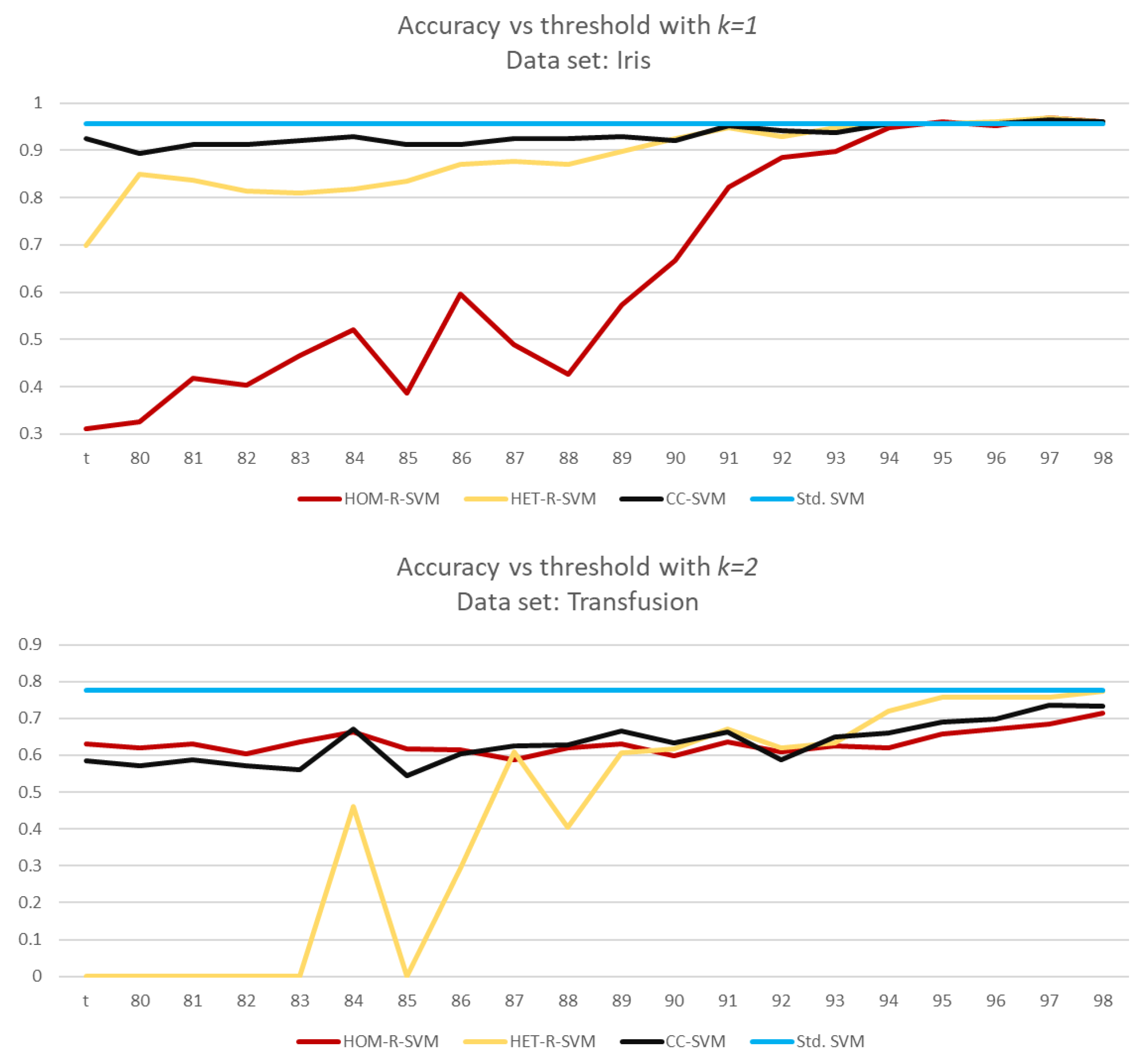
For a detailed analysis, we run another set of simulations from $t=0.80$ to $t=0.99$ with a step size of 0.01. In all data sets, CC-SVM is the most consistent algorithm. Two graphs below show how a SVM algorithm may fluctuate according to the data set.

For the Iris data set, HET-R-SVM and CC-SVM are consistent for $0.80\le t\le 0.99,$ but HOM-R-SVM gives reasonable accuracy for larger values of $t.$ With larger values of $t,$ the ratio $n_t/n$ also increases (see Figure 10).

This behavior, “fluctuating”, is not specific to HOM-R-SVM, as the Transfusion data set shows in Figure 10. HET-R-SVM does not give consistent accuracy values for $t<0.90$, even though HET-R-SVM gives the best accuracy for $t\ge 0.94.$ On the other hand, both HOM-R-SVM and CC-SVM are consistent for all values of $0.80\le t\le 0.99.$ Even though, the accuracy rates differ, as expected, the ratio $\frac{n_t}{t}$ is almost typical.

Both Figure 10 and Figure 11 show that for smaller values of $t,$ the number of examples used in SVM reduces significantly, whereas for larger values of t, more data are being used in SVM. Furthermore, depending on the distribution of the data, as seen for Transfusion data set in Figure 11, even for larger values of $t,$ there is still a reduction in the size of data before using SVM. This is also similar for the number of support vectors.

In conclusion, we proposed a new clustering algorithm based on cliques that can be used to discover relevant information for classification algorithms. Three different strategies for using the information obtained by the clique clustering algorithm were investigated. The results based on 10 real data sets obtained from the UCI repository [36] show that comparable accuracy performance can be obtained by these proposed algorithms with a smaller training data set size and fewer support vectors. In addition, the results indicate that each proposed classification algorithm can capture different aspects of the training data sets.

It is known that SVMs can have some problems with large data sets. For example, the performance of SVMs decrease significantly when the number of examples in the training data set increases ([37]). The results of this study show that the proposed classification algorithms are of potential use for investigating new classification strategies based on SVMs that can be used with large data sets.