Parallel Processing Method for Airborne Laser Scanning Data Using a PC Cluster and a Virtual Grid


Abstract
:
1. Introduction
2. Background
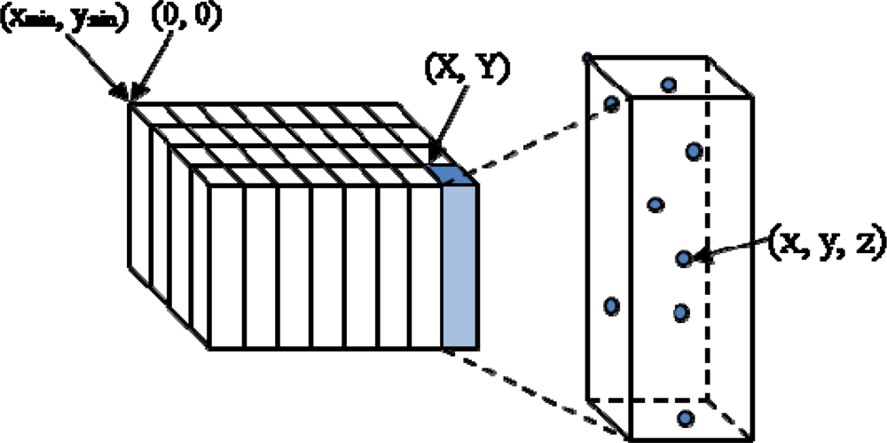
2.1. ALS Data Structure and Virtual Grid
2.2. Parallel processing and Performance Evaluation
2.2.1. Parallel Machines
2.2.2. Performance Evaluation
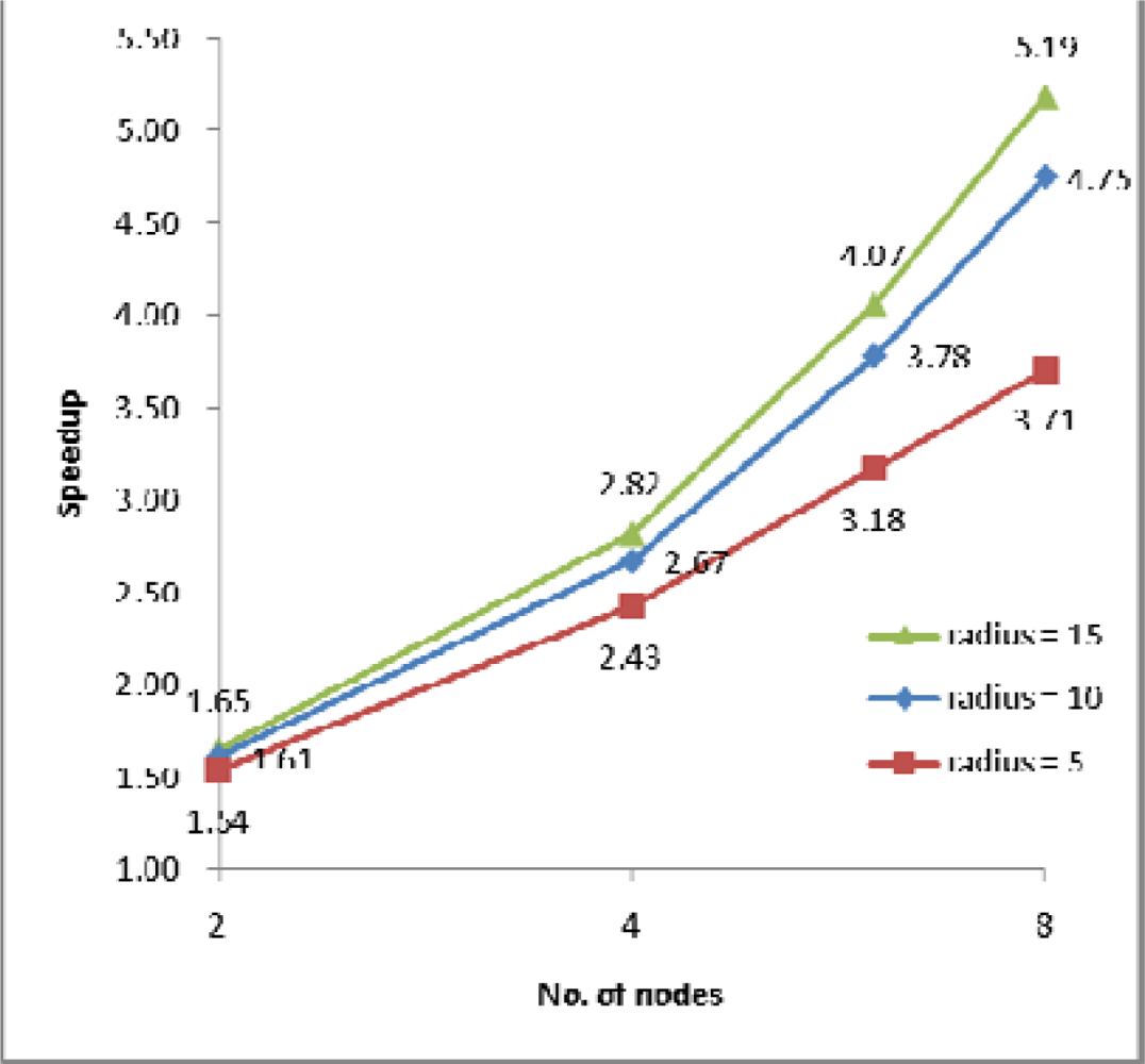
(1) Speedup
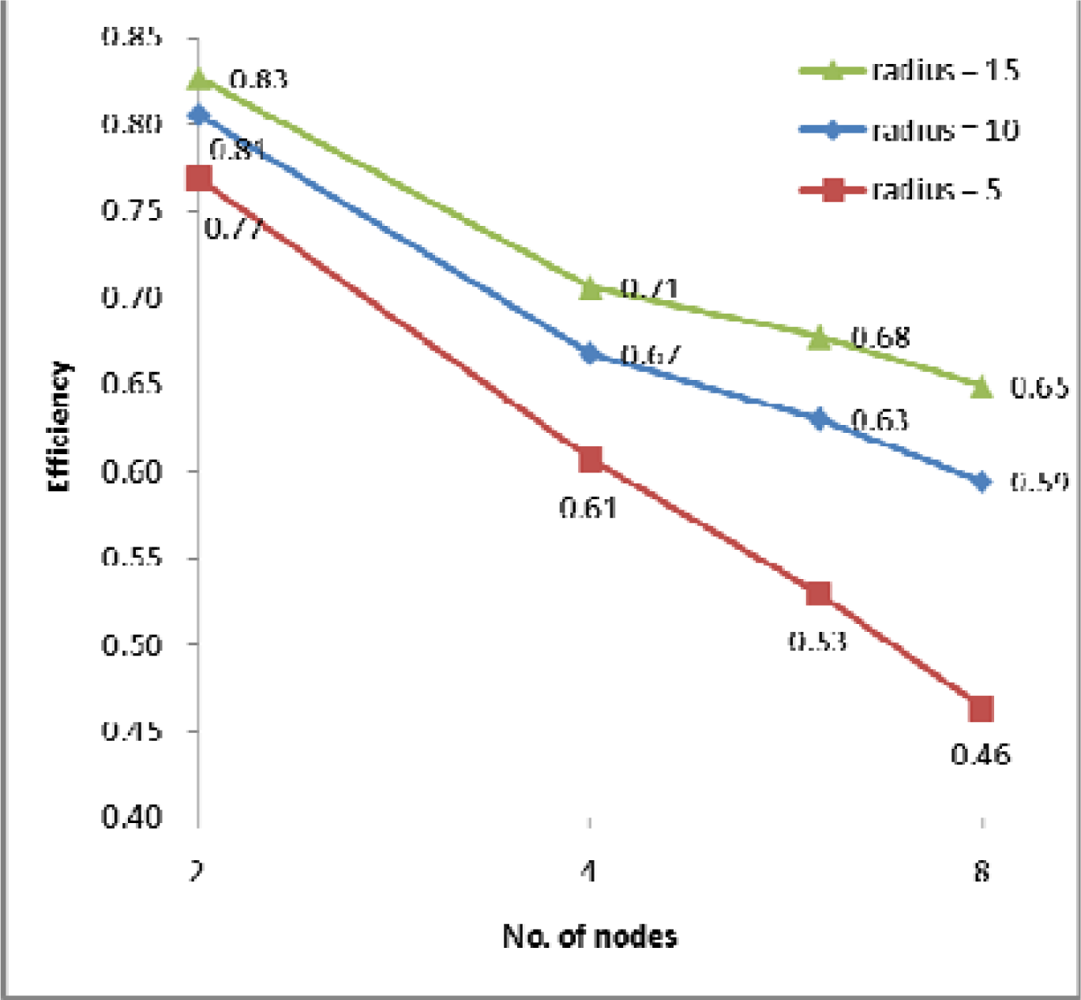
(2) Efficiency
(3) Load scalability and linearity
2.3. IDW and Local Minimum Filtering
3. Algorithm Development
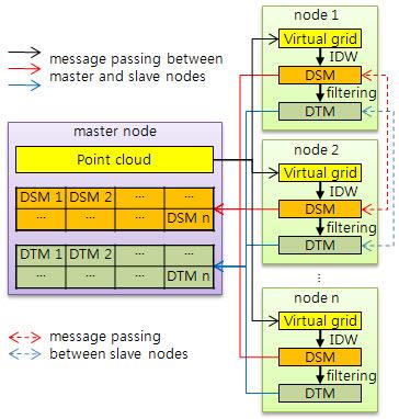
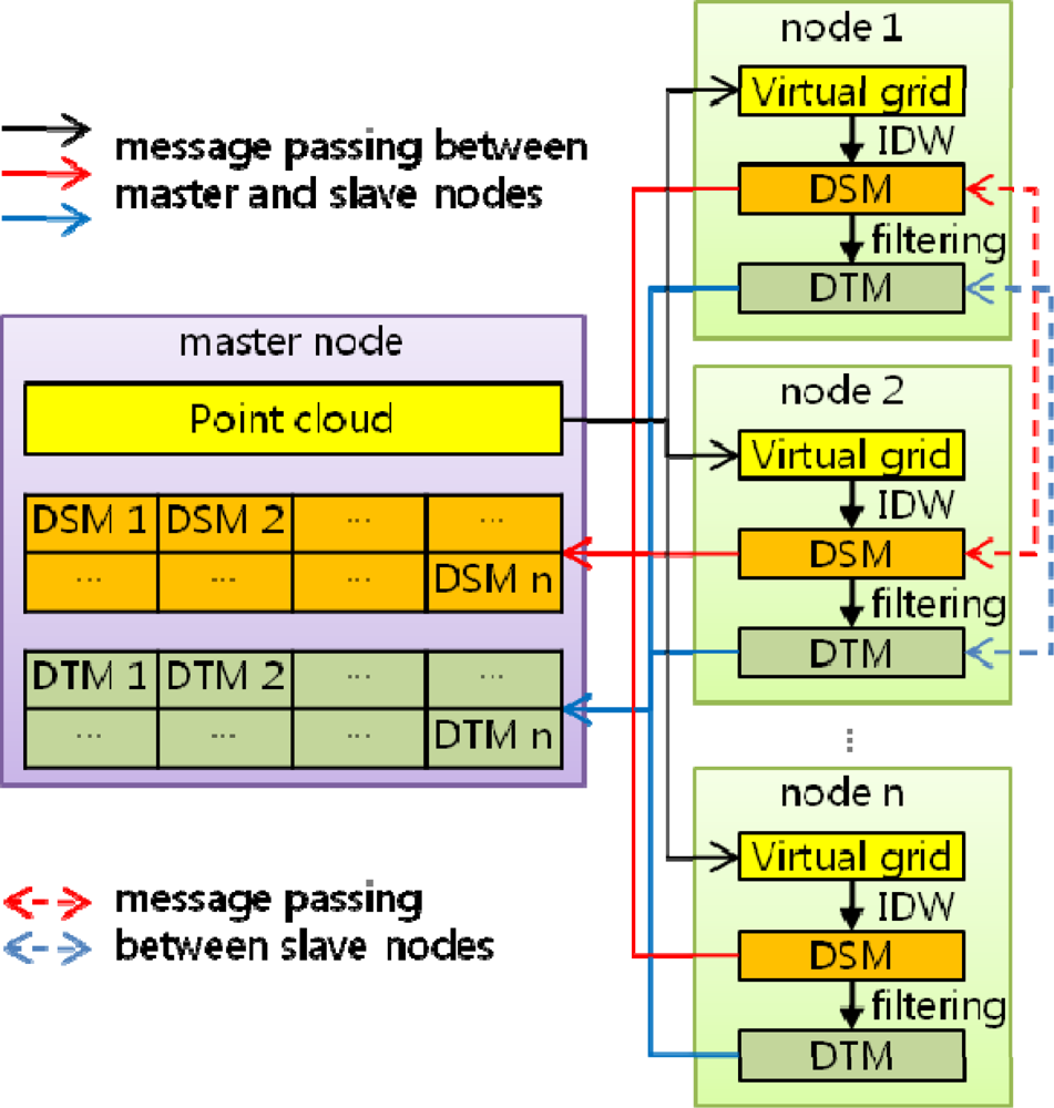
3.1. Overall Algorithm
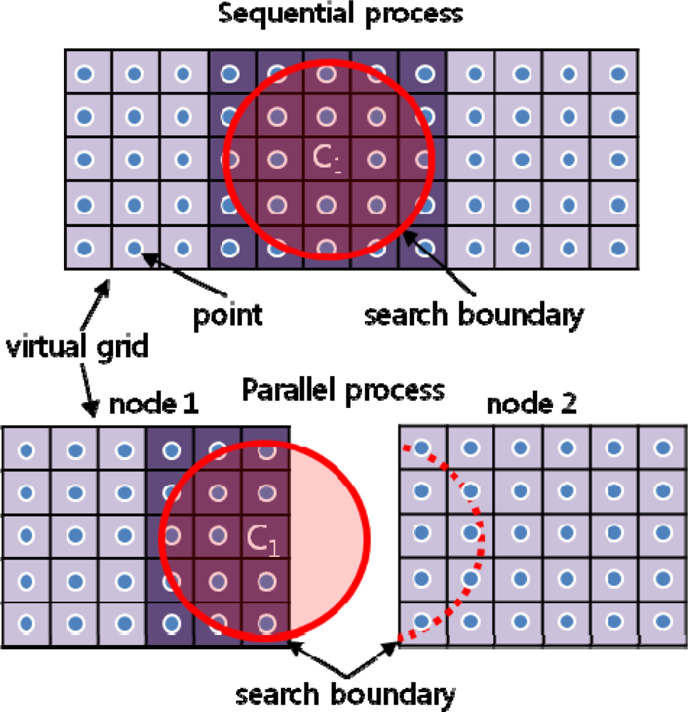
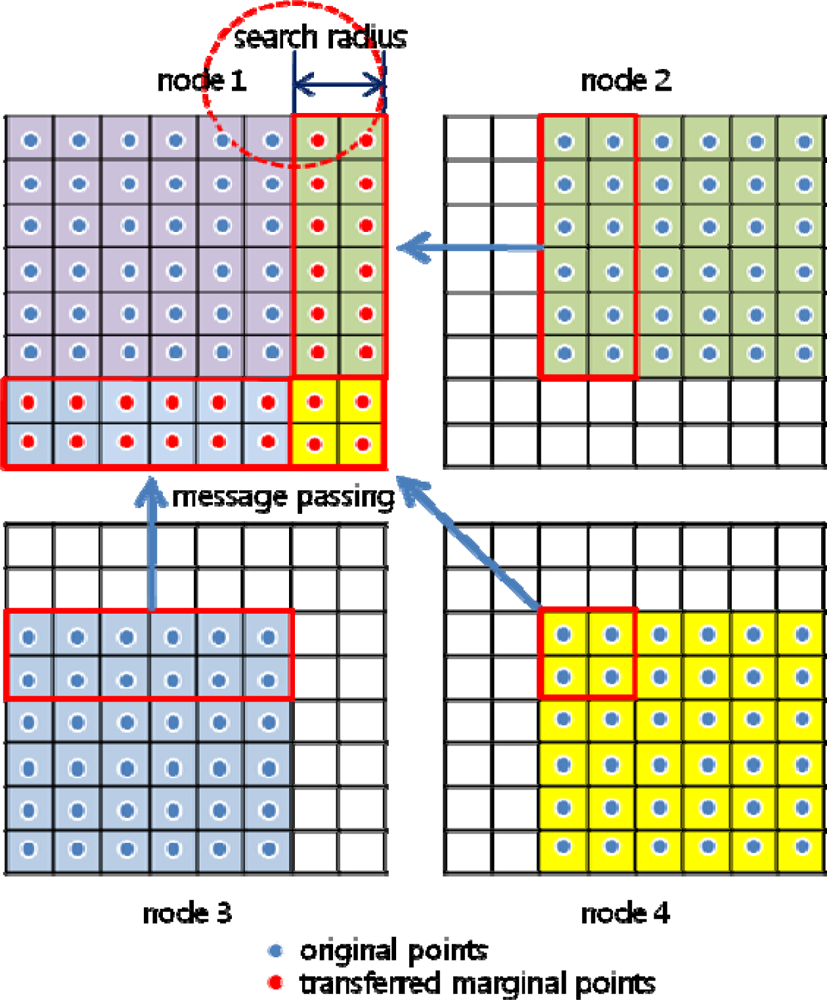
3.2. Boundary Problem
Method 1: Transferring data block allowing overlap of original data
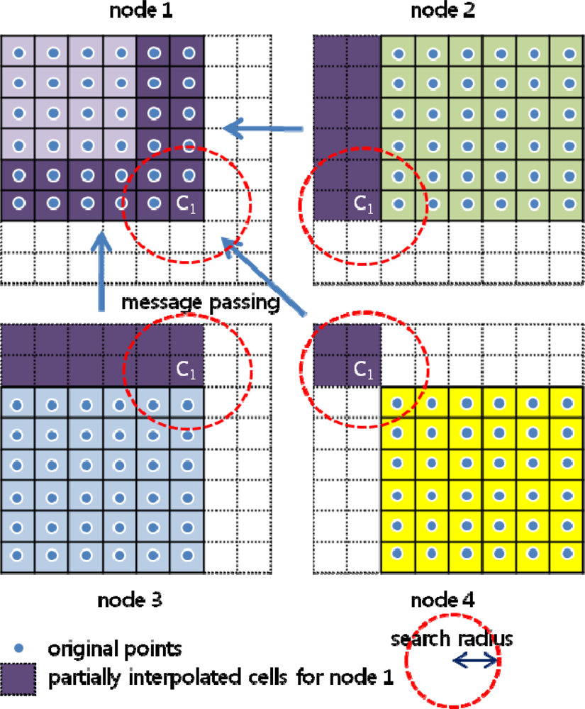
Method 2: Transferring partially interpolated value block without overlap of original data
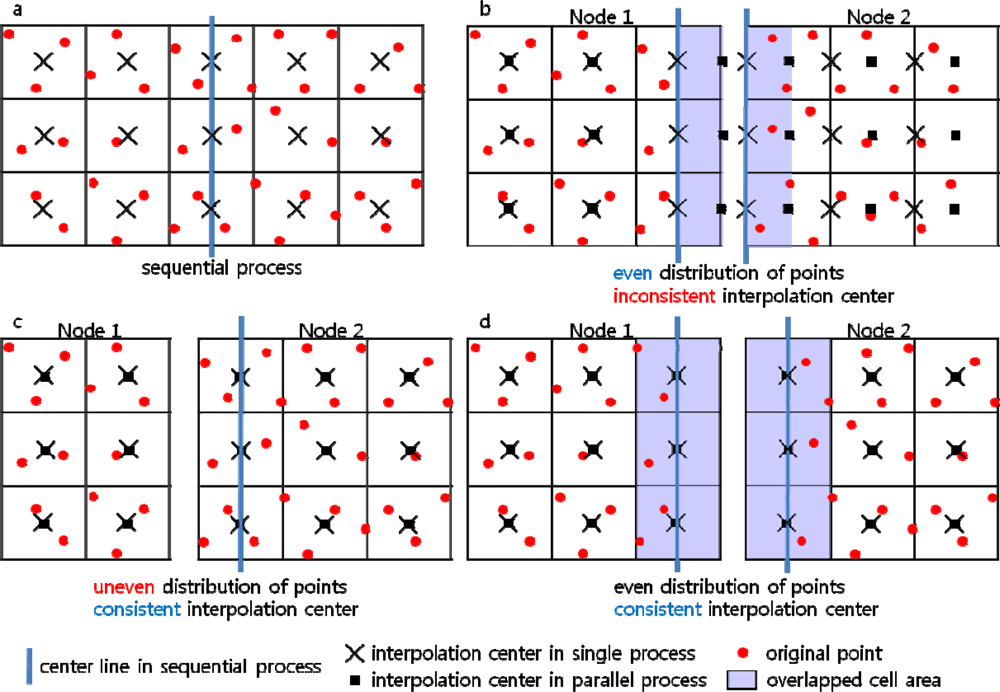
3.3 Interpolation Center Problem
Case A (Figure 7a)
Case B (Figure 7b)
Case C (Figure 7c)
Case D (Figure 7d)
4. Implementation and Discussion
4.1. Test Data and System Configuration
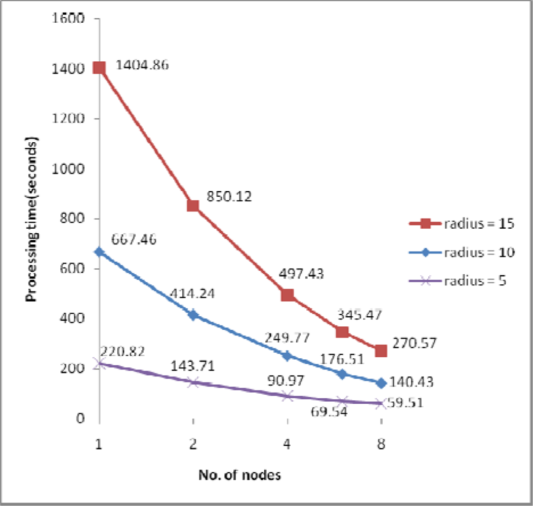
4.2. Performance Evaluation and Discussion
5. Conclusions
Acknowledgments
References and Notes
- Flood, M. Commercial Development of Airborne Laser Altimetry. Int. Arch. Photogramm. Remote Sens 1999, 32(3W14), 13–20. [Google Scholar]
- Baltsavias, E.P. A comparison between photogrammetry and laser scanning. ISPRS J. Photogramm. Remote Sens 1999, 54, 83–94. [Google Scholar]
- Shan, J.; Sampath, A. Urban DEM Generation from Raw LiDAR Data : a Labeling Algorithm and its Performance. Photogramm. Eng. Remote Sens 2005, 71, 217–226. [Google Scholar]
- Han, S.H.; Lee, J.H.; Yu, K.Y. An Approach for Segmentation of Airborne Laser Point Clouds Utilizing Scan-Line Characteristics. ETRI J 2007, 29, 641–648. [Google Scholar]
- Healey, R.; Dowers, S.; Gittings, B.; Mineter, M.J. Parallel Processing Algorithms for GIS; CRC Press: Basingstoke, UK, 1997. [Google Scholar]
- Clematis, A.; Mineter, M.; Marciano, R. High performance computing with geographical data. Parallel Comput 2003, 29, 1275–1279. [Google Scholar]
- Yang, C.; Hung, C. Parallel Computing in Remote Sensing Data Processing. Proceedings of ACRS, 2000.
- Plaza, A.J.; Chang, C. High Performance Computing in Remote Sensing; Chapman & Hall/CRC: Boca Raton, FL, USA, 2007. [Google Scholar]
- Wehr, A.; Lohr, U. Airborne laser scanning - an introduction and overview. ISPRS J. Photogramm. Remote Sens 1999, 54, 68–82. [Google Scholar]
- Cormen, T.H.; Leiserson, C.E.; Rivest, R.L.; Stein, C. Introduction to Algorithms, 2nd Ed ed; MIT Press: Cambridge, MA, USA, 2001. [Google Scholar]
- Han, S.H. Efficient segmentation of ALS point cloud utilizing scan line characteristic, Doctoral thesis.. Seoul National University, Seoul, Korea, 2008.
- Cho, W.; Jwa, Y.S.; Chang, H.J.; Lee, S.H. Pseudo-grid Based Building Extraction Using Airborne Lidar Data. Int. Arch. Photogramm. Remote Sens 2004, 35, 378–381. [Google Scholar]
- Quinn, M.J. Parallel programming in C with MPI and OpenMP; McGraw-Hill: Dubuque, IA, USA, 2004. [Google Scholar]
- Bader, D.A.; Pennington, R. Cluster computing: Applications. Int. J. High Perform. Comput 2001, 15, 181–185. [Google Scholar]
- Almeida, F.; Gomez, J.A.; Badia, J.M. Performance analysis for clusters of symmetric multiprocessors. Proceedings of 15th EUROMICRO International Conference on Parallel, Distributed and Network-Based Processing, Naples, Italy, 2007; pp. 121–128.
- Top 500 supercomputer sites. http://www.top500.org/ (last accessed on 24 Oct., 2008).
- Message Passing Interface. http://www-unix.mcs.anl.gov/mpi/ (last accessed on 24 Oct., 2008).
- Parallel Virtual Machine. http://www.csm.ornl.gov/pvm/ (last accessed on 24 Oct., 2008).
- JaJa, J. An Introduction to parallel algorithms; Addison-Wesley Publishing Company, Inc: Reading, MA, USA, 1992. [Google Scholar]
- Bondi, A.B. Characteristics of Scalability and Their Impact on Performance. Proceedings of Workshop on Software Performance, Ottawa, Canada, September 2000; pp. 195–203.
- Bartier, P.; Keller, C.P. Multivariate interpolation to incorporate thematic surface data using inverse distance weighting(IDW). Comput. Geosci 1996, 22, 795–799. [Google Scholar]
- García-León, J.; Felicísimo, A.M.; Martínez, J.J. A methodological proposal for improvement of digital surface models generated by automatic stereo matching of convergent image networks. Int. Arch. Photogramm. Remote Sens 1999, 35, 59–63. [Google Scholar]
- Gonçalves, G. Analysis of interpolation errors in urban digital surface models created from LIDAR data. Proceedings of the 7th International Symposium on Spatial Accuracy Assessment in Natural Resources and Environment Sciences, Lisbon, Portugal, 2006.
- Armstrong, M.P.; Marciano, R. Inverse-Distance-Weighted Spatial Interpolation Using Parallel Supercompters. Photogramm. Eng. Remote Sens 1994, 60, 1097–1103. [Google Scholar]
- Armstrong, M.P.; Marciano, R. Local Interpolation Using a Distributed Parallel supercomputer. Int. J. Geogr. Inf. Syst 1996, 10, 713–729. [Google Scholar]
- Clarke, K. C. Analytical and Computer Cartography; Prentice Hall: Englewood Cliffs, NJ, USA, 1990. [Google Scholar]
- Armstrong, M.P.; Marciano, R. Massively Parallel Strategies for Local Spatial Interpolation. Comput. Geosci 1997, 23, 859–167. [Google Scholar]
- Wang, S.; Armstrong, M.P. A Quadtree Approach to Domain Decomposition for Spatial Interpolation in Grid Computing Environments. Parallel Comput 2003, 29, 1481–1504. [Google Scholar]
- Rowland, C.S.; Balzter, H. Data Fusion for Reconstruction of a DTM, Under a Woodland Canopy, From Airborne L-band InSAR. IEEE Trans. geosci. remote sens 2007, 45, 1154–1163. [Google Scholar]
- Comer, D.E. Internetworking with TCP/IP Vol. 1, 2nd Ed ed; Pearson Prentice Hall: Upper Saddle River, NJ, USA, 2006. [Google Scholar]
- TerraSolid Ltd. Homepage. http://www.terrasolid.fi/ (last accessed on 24 Oct., 2008).


| Laser scanner | ALS ALTM 3070 system (Optech, Inc.) | |
| Target area | Daejeon, South Korea | |
| Preprocessing | Systematic error correction was applied. | Strip adjustment and blunder removal were not applied. |
| Dataset 1 | 4.8 × 10⁶ points covering1.5 × 0.8 km2 (3.7 points/m2) | cropped from dataset 6 |
| Dataset 2 | 9.4 × 10⁶ points covering 3.0 × 0.8 km2 (3.7 points/ m2) | cropped from dataset 6 |
| Dataset 3 | 17.9 × 10⁶ points covering 6.1 × 0.8 km2 (3.5 points/ m2) | cropped from dataset 6 |
| Dataset 4 | 31.7 × 10⁶ points covering 6.1 × 1.7 km2 (3.1 points/ m2) | cropped from dataset 6 |
| Dataset 5 | 79.3 × 10⁶ points covering 10.7 × 1.7 km2 (4.4 points/ m2) | cropped from dataset 6 |
| Dataset 6 | 133.7 × 10⁶ points covering 10.7 × 3.4 km2 (3.7 points/ m2) | full dataset |
| System configuration | Parallel Sequential | 1 master node with 1, 2, 4, 6, 8 slave nodes 1 node |
|---|---|---|
| Single Pentium 4 3.0 GHz, 1 GB RAM for each node | ||
| Network | 1Gb Ethernet | |
| Operating system | Windows XP sp3 | |
| MPI library | MPICH 2.0 (following MPI 2.0 standard) | |
| Coding language | C++ | |
| Virtual grid cell size | 1m by 1m |
| IDW search radius | 15m / 10m / 5m (for dataset 3), 10m (for other datasets) |
| IDW power | 2 |
| Filter size | 30m by 30m |
© 2009 by the authors; licensee MDPI, Basel, Switzerland This article is an open access article distributed under the terms and conditions of the Creative Commons Attribution license (http://creativecommons.org/licenses/by/3.0/).
Share and Cite
Han, S.H.; Heo, J.; Sohn, H.G.; Yu, K. Parallel Processing Method for Airborne Laser Scanning Data Using a PC Cluster and a Virtual Grid. Sensors 2009, 9, 2555-2573. https://doi.org/10.3390/s90402555
Han SH, Heo J, Sohn HG, Yu K. Parallel Processing Method for Airborne Laser Scanning Data Using a PC Cluster and a Virtual Grid. Sensors. 2009; 9(4):2555-2573. https://doi.org/10.3390/s90402555
Chicago/Turabian StyleHan, Soo Hee, Joon Heo, Hong Gyoo Sohn, and Kiyun Yu. 2009. "Parallel Processing Method for Airborne Laser Scanning Data Using a PC Cluster and a Virtual Grid" Sensors 9, no. 4: 2555-2573. https://doi.org/10.3390/s90402555
APA StyleHan, S. H., Heo, J., Sohn, H. G., & Yu, K. (2009). Parallel Processing Method for Airborne Laser Scanning Data Using a PC Cluster and a Virtual Grid. Sensors, 9(4), 2555-2573. https://doi.org/10.3390/s90402555