Sink-oriented Dynamic Location Service Protocol for Mobile Sinks with an Energy Efficient Grid-Based Approach

Abstract
:
1. Introduction
- We propose a global-grid structure to avoid repetitively constructing an individual grid structure for each source node. The global grid structure helps reduce overall energy consumption. A sink can use the global grid structure to identify the location of the source node whenever it wants to do so.
- We propose an Eight-Direction Anchor (EDA) system that acts as a location service server. EDA prevents intensive energy consumption at the border sensor nodes; consequently, the energy consumed is well balanced for all the sensor nodes.
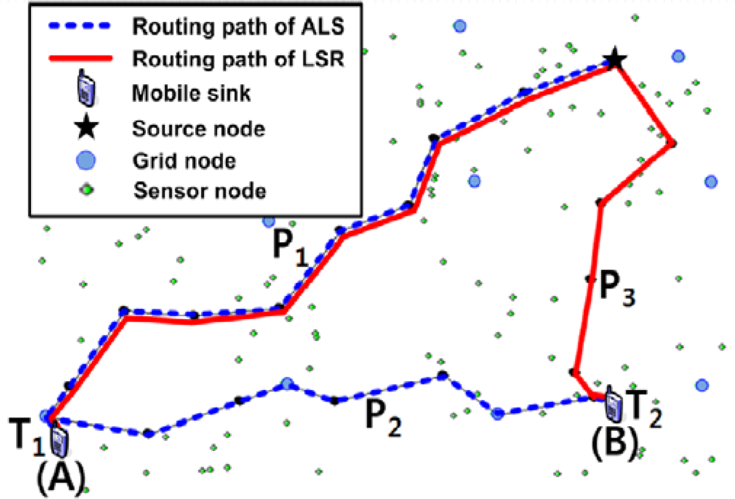
- We propose a Location-based Shortest Relay (LSR) that efficiently forwards (or relays) data from the source node to the sink with minimal path delay. Our protocol does not need a global grid structure anymore, once a sink identifies the location information of the source node by using global grid structure.
- We evaluate performance on a JAVA implementation of SDLS. We demonstrate that the proposed protocol not only reduces communication costs, but also balances energy consumption.
2. Related Work
2.1. Grid Structure Data Forwarding Approach with Mobile Sink
2.2. Location Service for a Location-based Approach with Mobile Sinks
3. Sink-oriented Dynamic Location Service
- Sensor nodes are placed in two-dimensional square field where they are randomly deployed with high density.
- Sensor nodes communicate with each other using single-hop communications through short-range radios. Long-range data delivery is accomplished forwarding data across multiple-hops.
- Each sensor node knows its own location, as well as the location of its 1-hop neighbor nodes using localization algorithms [25].
- Upon detecting an event of interest, a source node immediately reports its location information using the Eight-Direction Anchor (EDA) system.
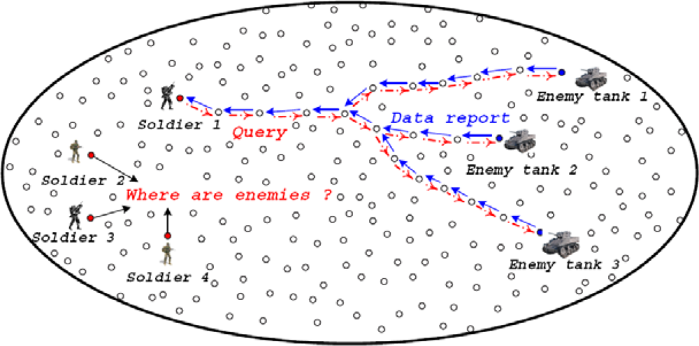
- One or more mobile sinks moves randomly in the deployment field. Sinks (users) query the network to collect the location of source nodes. Then, sinks wait until they receive the location of source nodes. After getting the location of the source node, the sink can dynamically send the data request query to the source node with consideration of source node’s location and direction of sink’s movement. Therefore, we named our proposed scheme as Sink-oriented Dynamic Location Service (SDLS) protocol.
3.1. Motivation
3.2. Global Grid Construction
3.3. Eight-Direction Anchor System
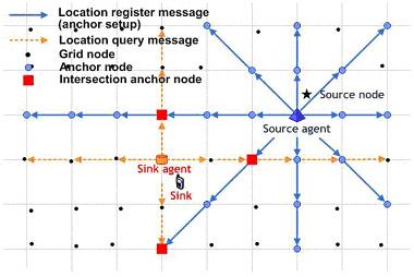
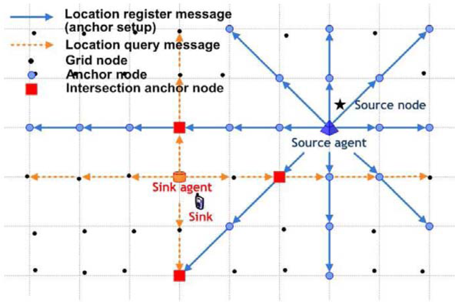
- Once an event occurs, a source node selects the nearest grid node as its source agent (see Figure 4, source node and selected source agent) and distributes the location information of the source node.
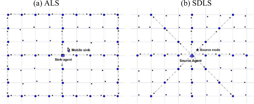
- The source agent broadcasts the location of the source node in eight directions (East, West, South, North, Northeast, Northwest, Southeast, and Southwest) through anchor setup messages.
- The anchor setup messages are relayed by intermediate sensor nodes between two neighboring grid nodes and the recruited anchors store a copy of the location of the source node.

| Procedure: |
| 01: initially startNode, middleNode, endNode = 0; |
| 02: source node finds the nearest grid node as source agent |
| /* source node floods a query within a local area about a cell size. */ |
| 03: startNode = source agent; |
| 04: for (source agent’s each neighbor grid node) /* to eight-direction */ |
| 05: endNode = neighbor grid node; |
| 06: while (endNode != border node) |
| 07: middleNode = forward (startNode, endNode); |
| /* finding the nearest neighbor node to reach the destination node */ |
| 08: if (middleNode == grid node) |
| 09: saveLocationServer (source node’s location information); |
| 10: end if |
| 11: startNode = middleNode; |
| 12: if (startNode == endNode) |
| 13: endNode = startNode.neighbor grid node; |
| /* i.e.) if the message is from the east, startNode’s neighbor grid node is same direction. */ |
| 14: end if |
| 15: end while |
| 16: end for |
3.4. Query and Data Dissemination
- The sink will register with the nearest grid node, known as the sink agent (see Figure 4, sink and selected sink agent).
- The sink agent sends four location query packets (East, West, South, and North) to find the location of the source node.
- The sink can obtain the location of source nodes from the location response at intersecting anchor nodes (Figure 4).
| Procedure: |
| 01: initially startNode, middleNode, endNode = 0; |
| 02: sink finds the nearest grid node as sink agent |
| /* sink floods a query within a local area about a cell size. */ |
| 03: startNode = sink agent; |
| 04: for (sink agent’s each neighbor grid node) /* to four-direction */ |
| 05: endNode = neighbor grid node; |
| 06: while (endNode != border node) |
| 07: middleNode = forward (startNode, endNode); |
| /* finding the nearest neighbor node to reach the destination node */ |
| 08: if (middleNode == grid node) |
| 09: if (exist a new source node’s location) |
| 10: getLocation (sink agent); /* reply to the sink */ |
| 11: end if |
| 12: end if |
| 13: startNode = middleNode; |
| 14: if (startNode == endNode) |
| 15: endNode = startNode.neighbor grid node; |
| /* i.e.) if the message is from the east, startNode’s neighbor grid node is same direction. */ |
| 16: end if |
| 17: end while |
| 18: end for |
3.5. Sink Mobility and Data Forwarding Maintenance
| Procedure: |
| 01: sink finds the nearest sensor node as sink primary agent |
| 02: if (source node receives query message from sink) |
| 03: source node sends data to sink |
| 04: end if |
| 05: if (source node continuously sends data to sink) |
| 06: if (sink is automatic operation) |
| 07: go to algorithm 3-1 |
| 08: end if |
| 09: if (sink is manual operation) |
| 10: go to algorithm 3-2 |
| 11: end if |
| 12: end if |
3.5.1. Automatic Operation
| Input: distance between source node and NPA |
| Output: shortest path in automatic operation |
| Parameter: |
| PA: Primary Agent, NPA: New Primary Agent |
| IA: Immediate Agent, NIA: New Immediate Agent |
| l1: distance between sink and PA (NPA) |
| l2: predefined distance (i.e. half of cell size) |
| l3: distance between PA and IA (NIA) |
| l4: predefined distance (i.e. three times of cell size) |
| l5: distance between source node and NPA via old PA |
| l6: predefined distance (i.e. two times of distance between source node and NPA) |
| Procedure: |
| 01: initially startFlag = true; |
| 02: do |
| 03: if (startFlag) |
| 04: if (l1 > l2) |
| 05: find IA and send IA’s location information to PA |
| 06: startFlag = false; |
| 07: end if |
| 08: end if |
| 09: else |
| 10: if (l1 > l2) |
| 11: if (l3 > l4) |
| 12: find NPA |
| 13: if (l5 > l6) |
| 14: update (NPA) /* update to source node */ |
| 15: end if |
| 16: end if |
| 17: end if |
| 18: else |
| 19: find NIA and send NIA’s location information to previous |
| 20: while (sink has mobility) |
3.5.2. Manual Operation
| Input: estimated distance between source node and sink |
| Output: shortest path in manual operation |
| Parameter: |
| PA: Primary Agent, NPA: New Primary Agent |
| Procedure: |
| 01: if sink wants to move far-away from PA /* close to source node */ |
| 02: sink sends stop message to source node |
| 03: if source node receives stop message |
| 04: source node saves data in its cache |
| 05: end if |
| 06: end if |
| 07: if sink wants to renew data |
| 08: sink finds NPA and sends query message to source node |
| 09: if source node receives query message |
| 10: source node sends data including stored data |
| 11: end if |
| 12: end if |
4. Performance Evaluation
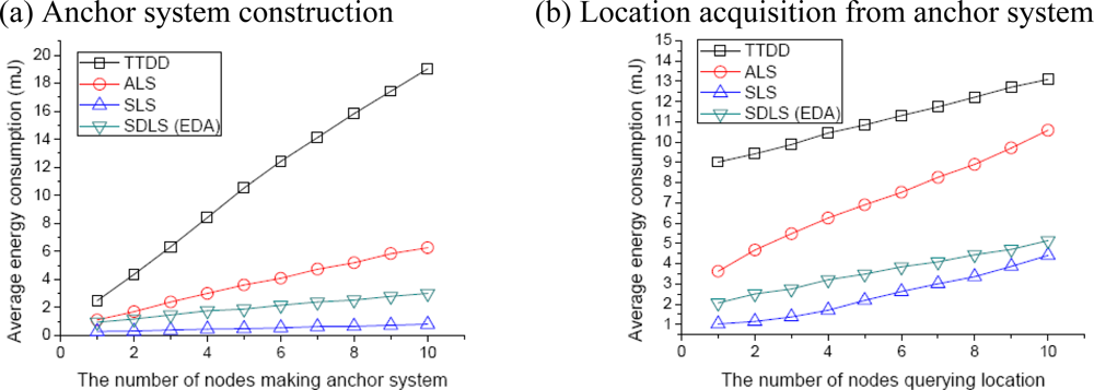
4.1. Average Energy Consumption for Location Service
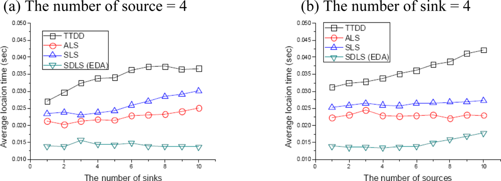
4.2. Location Response Time
4.3. Remaining Energy Power of the Sensor Nodes for Data Communication
4.4. Average Data Delivery Ratio
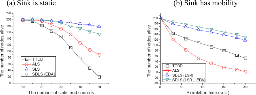
4.5. Network Lifetime
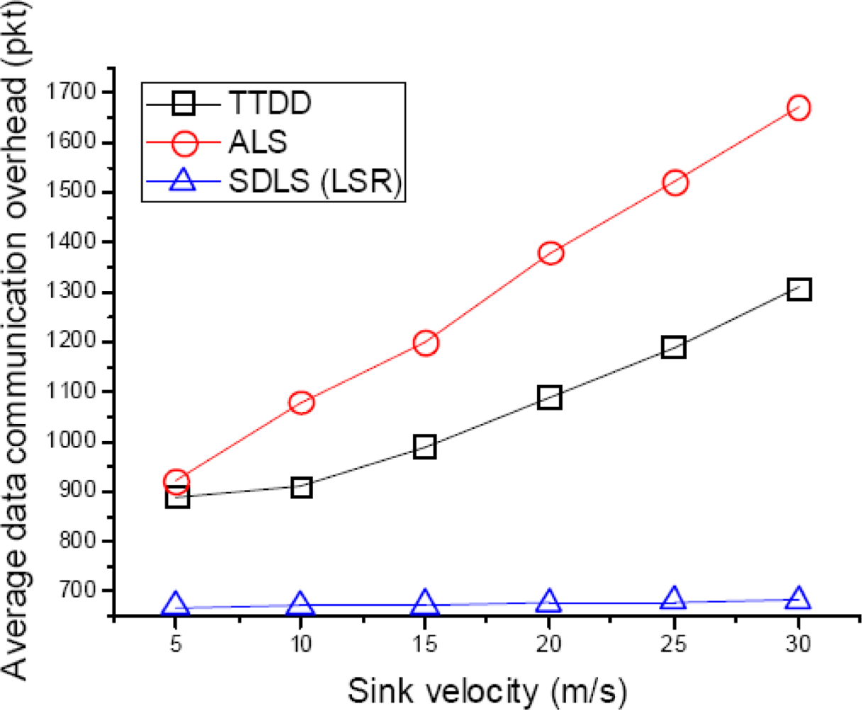
4.6. Average Data Communication Overhead
5. Conclusions
Acknowledgments
References and Notes
- Akyildiz, I.; Su, W.; Sankarasubramaniam, Y.; Cayirci, E. Wireless sensor networks: a survey. Comput. Networks 2002, 38, 393–422. [Google Scholar]
- Estrin, D.; Govindan, R.; Heidemann, J.; Kumar, S. Next century challenges: scalable coordination in sensor networks. ACM/IEEE International Conference on Mobile Computing and Networking (MOBICOM), Seattle, Washington, USA, August 1999; pp. 263–270.
- Jo, M.; Youn, H.Y.; Cha, S.H.; Choo, H. Mobile RFID Tag Detection Influence Factors and Prediction of Tag Detectability. IEEE Sens. J 2009, 9, 112–119. [Google Scholar]
- Heinzelman, W.R.; Kulik, J.; Balakrishnan, H. Adaptive protocols for information dissemination in wireless sensor networks. ACM/IEEE International Conference on Mobile Computing and Networking (MOBICOM), Seattle, Washington, USA, August 1999; pp. 174–185.
- Heinzelman, W.R.; Chandrakasan, A.; Balakrishnan, H. Energy-efficient communication protocol for wireless microsensor networks. IEEE Hawaii International Conference System Sciences (HICSS), Hawaii, USA, January 2000; pp. 20–30.
- Liu, M.; Cao, J.; Chen, G.; Wang, X. An Energy-Aware Routing Protocol in Wireless Sensor Networks. Sensors 2009, 9, 445–462. [Google Scholar]
- Park, S.; Shin, K.; Abraham, A.; Han, S. Optimized Self Organized Sensor Networks. Sensors 2007, 7, 730–742. [Google Scholar]
- Wang, G.; Wang, H.; Cao, J.; Guo, M. Energy-Efficient Dual Prediction-Based Data Gathering for Environmental Monitoring Applications. IEEE Wireless Communications and Networking Conference (WCNC), Hong Kong, China, March 2007; pp. 3513–3518.
- Intanagonwiwat, C.; Govindan, R.; Estrin, D. Directed diffusion: a scalable and robust communication paradigm for sensor networks. ACM/IEEE International Conference on Mobile Computing andNetworking (MOBICOM), Boston, Massachusetts, USA, August 2000; pp. 56–67.
- Park, K.; Choo, H. Energy-Efficient Data Dissemination Schemes for Nearest Neighbor Query Processing. IEEE Trans. Comput 2007, 56, 754–768. [Google Scholar]
- Kim, S.; Son, S.; Stankovic, J.; Li, S.; Choi, Y. SAFE: a data dissemination protocol for periodic updates in sensor networks. IEEE Distributed Computing Systems Workshops, Providence, Rhode Island, USA, May 2003; pp. 228–234.
- Kim, H.S.; Abdelzaher, T.F.; Kwon, W.H. Minimum-energy asynchronous dissemination to mobile sinks in wireless sensor networks. ACM International Conference on Embedded Networked Sensor Systems, LosAngeles, California, USA, November 2003; pp. 193–204.
- Huang, Q.; Bai, Y.; Chen, L. An Efficient Route Maintenance Scheme forWireless Sensor Network with Mobile Sink. IEEE Vehicular Technology Conference (VTC), In the capital of the Celtic Tiger, Dublin, April 2007; pp. 155–159.
- Zhou, Z.; Xang, X.; Wang, X.; Pan, J. An Energy-Efficient Data-Dissemination Protocol inWireless Sensor Networks. IEEE International Symposium on a World of Wireless, Mobile and Multimedia Networks (WoWMoM), Buffalo, NY, USA; 2006; pp. 10–19. [Google Scholar]
- Hornsberger, J.; Shoja, G.C. Geographic grid routing for wireless sensor networks. IEEE Networking, Sensing and Control, Tucson, Arizona, USA, March 2005; pp. 484–489.
- Luo, H.; Ye, F.; Cheng, J.; Lu, S.; Zhang, L. TTDD: A Two-tier Data Dissemination Model for Large-ScaleWireless Sensor Networks. ACM/IEEE International Conference on Mobile Computing and Networking (MOBICOM), Atlanta, Georgia, USA, September 2002; pp. 148–159.
- Li, J.; Jannotti, J.; Couto, D.; De; Karger, D.; Morris, R. A scalable location service for geographic ad-hoc routing. ACM/IEEE International Conference on Mobile Computing and Networking (MOBICOM), Boston, Massachusetts, USA, August 2000; pp. 120–130.
- Das, S.M.; Pucha, H.; Hu, Y.C. Performance comparison of scalable location services for geographic ad hoc routing. IEEE 24th Annual Joint Conference of the IEEE Computer and Communications Societies (INFOCOM), Miami, USA, March 2005; pp. 1228–1239.
- Akkaya, K.; Younis, M.; Bangad, M. Sink Repositioning for Enhanced Performance in Wireless Sensor Networks. Comput. Networks 2005, 49, 512–534. [Google Scholar]
- Shim, G.; Park, D. Locators of Mobile Sinks for Wireless Sensor Networks. International Conference Workshops on Parallel Processing (ICPPW), Columbus, Ohio, USA, August 2006; pp. 159–164.
- Shin, J.H.; Kim, J.; Park, K.; Park, D. Railroad: virtual infrastructure for data dissemination in wireless sensor networks. ACM International Workshop on Performance Evaluation of Wireless Ad Hoc, Sensor, and Ubiquitous Networks (PE-WASUN), Montreal, Quebec, Canada, October 2005; pp. 168–174.
- Yan, Y.; Zhang, B.; Mouftah, H.T.; Ma, J. Hierarchical Location Service for Large Scale Wireless Sensor Networks with Mobile Sinks. IEEE Global Telecommunications Conference (GLOBECOM), Washington, DC, USA, November 2007; pp. 1222–1226.
- Zhang, R.; Zhao, H.; Labrador, M.A. The Anchor Location Service (ALS) Protocol for Large-scale Wireless Sensor Networks. ACM International Conference on Integrated Internet Ad hoc and Sensor Networks (InterSense), Nice, France, May 2006; pp. 18–27.
- Yu, F.; Choi, Y.; Park, S.; Lee, E.; Jin, M.S.; Kim, S.H. Sink Location Service for Geographic Routing in Wireless Sensor Networks. IEEE Wireless Communications and Networking Conference (WCNC), Las Vegas, USA, March 2008; pp. 2111–2116.
- Albowicz, J.; Chen, A.; Zhang, L. Recursive position estimation in sensor networks. Proceedings of IEEE ICNP, Riverside, California, USA, November 2001; pp. 35–41.
- Karp, B.; Kung, H.T. Greedy Perimeter Stateless Routing for Wireless Networks. ACM/IEEE International In Conference on Mobile Computing and Networking (MOBICOM), Boston, Massachusetts, USA, August 2000; pp. 243–254.
- Bhardwaj, M.; Garnett, T.; Chandrakasan, A.P. Upper bounds on the lifetime of sensor networks. IEEE International Conference on Communications (ICC), Helsinki, Finland, June 2001; pp. 785–790.
- Camp, T.; Boleng, J.; Davies, V. A Survey of Mobility Models for Ad Hoc Network Research. Wireless Commun. Mobile Comput 2002, 2, 483–502. [Google Scholar]


| Network size | 1000 m × 1000 m |
| α11, α12 | 80 nJ/bit |
| α2 | 100 pJ/bit/m2 |
| Packet size (control, data) | 36 bytes, 64 bytes |
| Transmission range | 200 m |
| Distribution type of sensor nodes | uniform |
| Model of the sink mobility | Random way-point |
© 2009 by the authors; licensee MDPI, Basel, Switzerland This article is an open-access article distributed under the terms and conditions of the Creative Commons Attribution license (http://creativecommons.org/licenses/by/3.0/).
Share and Cite
Jeon, H.; Park, K.; Hwang, D.-J.; Choo, H. Sink-oriented Dynamic Location Service Protocol for Mobile Sinks with an Energy Efficient Grid-Based Approach. Sensors 2009, 9, 1433-1453. https://doi.org/10.3390/s90301433
Jeon H, Park K, Hwang D-J, Choo H. Sink-oriented Dynamic Location Service Protocol for Mobile Sinks with an Energy Efficient Grid-Based Approach. Sensors. 2009; 9(3):1433-1453. https://doi.org/10.3390/s90301433
Chicago/Turabian StyleJeon, Hyeonjae, Kwangjin Park, Dae-Joon Hwang, and Hyunseung Choo. 2009. "Sink-oriented Dynamic Location Service Protocol for Mobile Sinks with an Energy Efficient Grid-Based Approach" Sensors 9, no. 3: 1433-1453. https://doi.org/10.3390/s90301433
APA StyleJeon, H., Park, K., Hwang, D.-J., & Choo, H. (2009). Sink-oriented Dynamic Location Service Protocol for Mobile Sinks with an Energy Efficient Grid-Based Approach. Sensors, 9(3), 1433-1453. https://doi.org/10.3390/s90301433