Feature Reduction in Graph Analysis

Abstract
:1. Introduction
2. Medical Image Feature Survey
3. Feature Domains
- Energy or angular second moment (an image homogeneity measure):
- Entropy:
- Maximum probability:
- Contrast:
- Inverse difference moment:
- Correlation (a measure of image linearity, linear direction structures in direction ϕ where μx, μy, σx, σy are means and standard deviations.
- Spectral entropy:
- Block activity: where i, j are window size and
4. Methodology
4.1. Feature classification
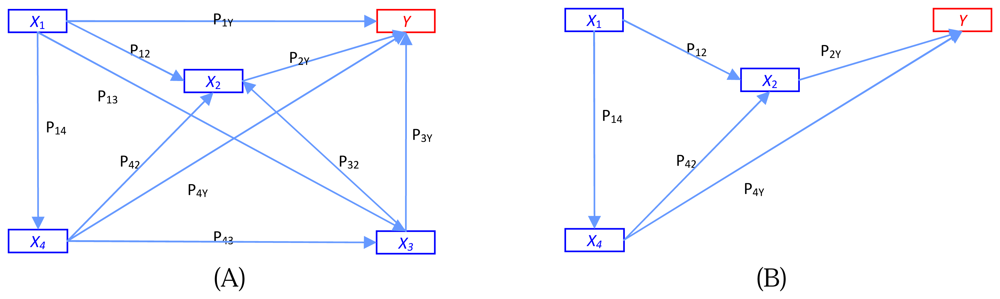
4.2. Path analysis
4.3. Relations among features and outputs
- a)
- a) Using logistic regression. Logistic regression is a regression model for Bernoulli-distributed dependent variables. It is a linear model that utilizes the logit as its link function. Logistic regression has been used extensively in medical and social sciences [4, 11]. The logit model takes the form:where pi=Pr(yi=1), βj>0; j =1, 2 … k are parameters (weight) of feature xi and ei is a random error (bias) of feature vector of a sample data.Logistic regression model can be used to predict the response features to be 0 or 1 (benign or malignant in the case of mammogram detection). Rather than classifying an observation into one group or the other, logistic regression predicts the probability p of being in either group. The model predicts the log odds (p/(1-p)) that an observation later be transformed to p as value of 0 or 1 with an optimal threshold. The general prediction model is log(p/(1-p)) = xβ+ϵ, where x is feature vector; β is a parameter vector; and ϵ is a random error vector.
- b)
- Using simple regression and multiple regression. Simple regression has the same basic concepts and assumptions as logistic regression but the dependent variable is continuous and the model has only a single independent variable. The simple regression can be modeled as Yi = β0 +β1X1i + ei ;i =1,2…n where Yi is the dependent variable, β0 , Regression yields a p value for the estimator ofβ1 are parameters (weights), and n is the size of training data. X1i is an explained variable of data record i and ei is a random error. Regression yields a p value for the estimator of Perform simple logistic regression β1 that can be used to decide whether Y has a linear relation to X . Multiple regression is an extension of simple regression model to multiple variables.
4.4. Hypothesis testing
5. Proposed Algorithm
- Step 1:
- Partition the original feature sets (x1, x2 … xn) into subsets using coefficients of the correlation matrix. Let the feature subsets be Si = (x1i, x2i … xji), i=1, 2 … k with pij being the correlation coefficient between xi and xj.This step is to partition all features into feature subsets Si, where Si and Sj (i≠j) are lowly dependent based on the correlations.
- Step 2:
- Perform simple logistic regression of each independent feature xji ϵ Si, j=1, 2 … Ri and dependent output y and then select the possible solution which satisfies a threshold value P.The result from this step is a subset Ai = (xri, xpi … xki) of features from Si is where each element of Ai is a direct causal feature of output y.
- Step 3:
- Perform multiple logistic regression by using all features in set Si, i=1, 2 … k in the model and selecting the signified features Bi = (xti, xli … xzi) from the model, where Bi is a set of direct features and indirect cause features.
- Step 4:
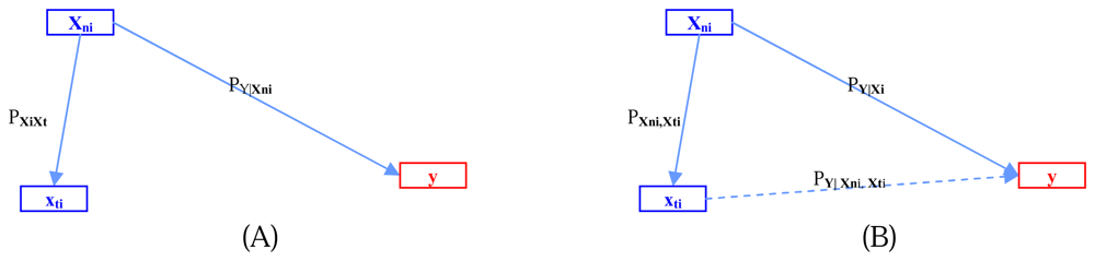
- Let Di = Ai Ə Bi; where Ə is our testing hypothesis operator for exploring the causal relations using the Bayesian inference conceptual framework.This step is performed using Bayesian inference as in the following example for two features:where C is a given thresholdThis step iteratively refines the search for the indirect cause feature with the highest correlation with the direct cause xmi.Through the above predicates (1) to (4), we can accept the hypothesis that xni and the combination of xni and xti cause y. Figure 2 illustrates the relations among xni, xti, and y.
- Step 5:
- Repeat from Step 2 while i ≤ k. This step produces sets Di, where i=1, 2 … k. Note that some of Di may be null sets.
- Step 6:
- Construct graph G by merging subgraphs Di; i=1, 2 … k;G(V, E | Y) = ∪ki=1Di;V = (vi); E = (ei); Y is the effect or dependent vertex.
6. Experiment and Results
6.1. Experiment
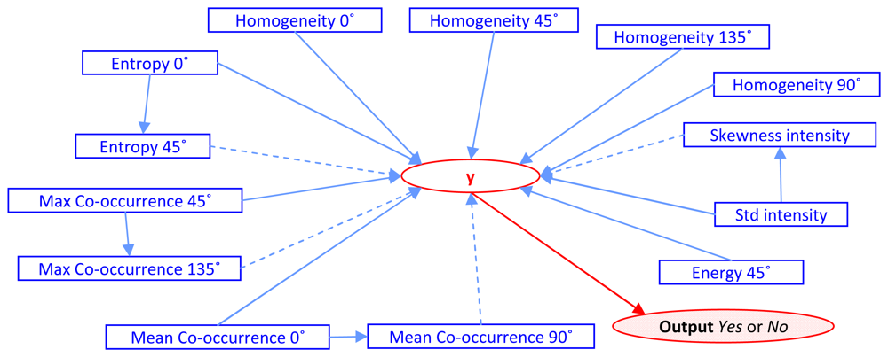
- From Table 3: Entropy 0° and Entropy 45° are highly significantly related.
- From the second column of Table 4: based on the simple logistic model, only Entropy 0° causes y (Entropy 0° is significant to y).
- From the third column of Table 4: on the multiple logistic regression model, Entropy 0° and Entropy 45° cause y.
- Finally, with Bayes inference, the direct effect is Entropy 0° and the indirect effect is the interaction of Entropy 0° and Entropy 45° cause y.
6.2. Verification
6.3. Analysis of results
7. Conclusions
Acknowledgments
References
- Hiroyuki, A.; Herber, M.; Junji, S.; Qing, L.; Roger, E.; Kunio, D. Computer – Aided Diagnosis in Chest Radiography: Results of Large –Scale Observer Tests at the 1886-2001 RSNA Scientific Assemblies. Radiographics 2003, 23, 255–265. [Google Scholar]
- Cosit, D.; Loncaric, S.L. Ruled Based Labeling of CT head Image. Proc. 6th Conference on Artificial Intelligence in Medicine, Europe; 1997; pp. 453–456. [Google Scholar]
- Gliman, D.M.; Sizzanme, L. State of the Art FDG Pet Imaging of Lung Cancer. Semin. Roentgenol. 2005, 40, 143–153. [Google Scholar]
- Dodd, L.E.; Wagner, R.F.; Armato, S.G.; McNitt-Gray, M.F.; Beiden, S.; Chan, H.P.; Gur, D.; McLennan, G.; Metz, C.E.; Petrick, N.; Sahiner, B.; Sayre, J. Assessment Methodologies and Statistical Issues for Computer-Aided Diagnosis of Lung Nodules in Computed Tomography. Acad. Radiol. 2004, 11, 462–474. [Google Scholar]
- Almato, G.S.; Roy, A.S.; MacMahon, H.; Li, F.; Doi, K.; Sone, S.; Altman, M.B. Evaluation of Automated Lung Nodule Detection on Low dose Computed Tomography Scan From a Lung Cancer Screening Program. AUR. Acad. Radiol. 2005, 12, 337–346. [Google Scholar]
- Chiou, G.I.; Hwang, J.-N. A Neural Network Based Stochastic Active Nodule (NNS-SNAKE) for Contour Finding of Distinct Features. Image Process. IEEE Trans. 1995, 4, 1407–1416. [Google Scholar]
- Goodman, L.A. Exploratory latent structure analysis using both identifiable and unidentifiable models. Biometrica 1971, 61, 215–231. [Google Scholar]
- Hagenarrs, J.A. Categorical causal modeling latent class analysis and discrete log-linear models with latent variables. Sociol. Methods Res. 1998, 26, 436–486. [Google Scholar]
- Lung Cancer Home Page. http://www.lungcancer.org/patients/fs_pc_lc_101.htm December 25, 2007.
- Guler, I.; Ubeyli, E.D. Expert systems for time-varying biomedical signals using eigen vector methods. Expert Syst. Appl. 2007, 32, 1045–1058. [Google Scholar]
- Song, J.H.; Venkatesh, S.S.; Conant, E.A.; Arger, P.H.; Sehgal, C.M. Comparative Analysis of Logistic Regression and Artificial Neural Network for Computer-Aided Diagnosis of Breast Masses. Acad. Radiol. 2005, 12, 487–495. [Google Scholar]
- Shiraishi, J.; Abe, H.; Li, F.; Engelmann, R.; MacMahon, H.; Doi, K. Computer-aided Diagnosis for the Detection and Classification of Lung Cancers on Chest Radiographs. Science Direct. Acad. Radiol. 2006, 13, 995–1003. [Google Scholar]
- Fu, J.C.; Lee, S.K.; Wong, S.T.C.; Yeh, J.Y.; Wang, A.H.; Wu, H.K. Image segmentation feature selection and pattern classification for mammographic microcalcifications. Comput. Med. Image 2005, 29, 419–429. [Google Scholar]
- Joreskog, K.G.; Sorbom, D. LISRL 7 User's Reference Guide; SPSS Inc.: Chicago, 1989. [Google Scholar]
- Doi, K.; MacMahon, H.; Katsuragawa, S.; Nishikawa, R.M.; Jiang, Y. Computer-aided diagnosis in radiology: Potential and pitfall. Eur. J. Radiol. 1999, 31, 97–109. [Google Scholar]
- Zhao, L.; Boroczky, L.; Lee, K.P. False positive reduction for lung nodule CAD using support vector machines and genetic algorithms. Comput. Assist. Radiol. Surg. 2005, 1281, 1109–1114. [Google Scholar]
- Lehmann, T.M.; Guld, M.O.; Thres, C.; Fischer, B.; Spitzer, K. Content-Based Access to Medical Images. http://phobos.imib.rwth-aachen.de/irma/ps-pdf/MI2006_Resubmission2.pdf.
- Miller, H.; Marquis, S.; Cohen, G.; Poletti, P.A.; Lovis, C.; Geissbuhler, A. Automatic: Abnormal Region detection in Lung CT images for Visual Retrieval. University and Hospital of Geneva, Service of Medical Informatics, Department de Radiologie et Informatique Medicale Home Page. http://www.simhcuge.ch/medgift September 5, 2007.
- Pietikainen, M.; Ojala, T.; Xu, Z. Rotation Invariant Texture Classification Using Feature Distributions. available online: www.mediateam.oulu.fi/publications/pdf/7.
- Foggia, P.; Guerriero, M.; Percannella, G.; Sansone, C.; Tufano, F.; Vento, M. A Graph-Based Method for Detecting and Classifying Clusters in Mammographic Images. Lect. Notes Comput. Sci., Struct. Syntact. Stat. Patt. Recog. 2006, 4109, 484–493. [Google Scholar]
- Zhang, P.; Verma, B.; Kumar, K. Neural Vs Statistical Classifier in Conjunction with Genetic Algorithm Feature Selection in Digital Mammography. Proc. 2004 IEEE Int. Joint Conf.Neural Networks; 2004; 3, pp. 2303–2308. [Google Scholar]
- Jiang, W.; Li, M.; Zhang, H.; Gu, J. Online Feature Selection Based on Generalized Feature Contrast Model. IEEE Int. Conf. Multimedia Expo (CME) 2004. [Google Scholar]
- Widodo, A.; Yang, B.-S. Application of nonlinear feature extraction and support vector Machines for fault diagnosis of induction motors. Expert Syst. Appl. 2007, 33, 241–250. [Google Scholar]
- Songyang, Y.; Ling, G. A CAD System for the Automatic Detection of Clustered Microcalcifications in Digitized Mammogram Films. IEEE T. Med. Imaging 2000, 19, 115–126. [Google Scholar]
- Yang, B.S.; Han, T.; Hwang, W. Application of multi-class support vector rotating machinery. J. Mech. Sci. Tech. 2005, 19, 845–858. [Google Scholar]
- Chiou, Y.; Lure, Y.; Ligomenides. Neural network image analysis and Classification in hybrid lung nodule detection (HLND) system. Proc. IEEE -SP Workshop Neural Networks Signal Process; 1993; pp. 517–526. [Google Scholar]
- Zhao, W.; Yu, X.; Li, F. Microcalcification Patterns Recognition Based Combination of Auto association and Classifier. Lect. Notes Comput. Sci., Comput. Intell. Secur. 2005, 3801, 1045–1050. [Google Scholar]
- Zheng, B.; Qian, W.; Clarke, L.P. Digital mammography: mixed feature neural network with spectral entropy decision for detection of microcalcifications. IEEE T. Med. Imaging 1996, 15, 589–97. [Google Scholar]
- Liang, Z.; Jaszczak, R.J.; Coleman, R.E. Parameter Estimation of Finite Mixtures Using the EM Algorithm and Information Criteria with Application to Medical Image Processing. IEEE T. Nucl. Sci. 1992, 39, 1126–1133. [Google Scholar]
- Majcenic, Z.; Loncaric, S. CT Image Labeling Using Simulated Annealing Algorithm. http://citeseerx.ist.psu.edu accessed July 12, 2007.


| Researcher | Domain | Features used (examples) | Classifier |
|---|---|---|---|
| Fu et al. [13] | Texture | Co-occurrence matrix rotation with angle 0°, 45°, 90°, 135°: Difference entropy, entropy, difference variance, contrast, angular second moment, correlation | GRNN (SFS, SBS) |
| Spatial | Mean, area, standard deviation, foreground/ background ratio, area, shape moment intensity variance, energy –variance | ||
| Spectral | Block activity, Spectral entropy | ||
| G. Samuel et al. [5] | Spatial | Volume, sphericity, mean gray level, gray level standard deviation, gray level threshold, radius of sphere, maximum eccentricity, maximum circularity, maximum compactness | Rule-based, linear discriminant analysis |
| E. Lori et al. [4] | Spatial, Patient Profile | Patient profile, nodule size, shape (measured with ordinal scale) | Regression analysis |
| Shiraishi et al. [12] | Multi Domain | Patient profile, root-mean-square of power spectrum,histograms frequency, full width at half maximum of the histogram for the outside region of the segmented nodule on the background–corrected image, degree of irregularity, full width at half maximum for inside region of segmented nodule on the original image | Linear discriminant analysis |
| Hening [18] | Spatial | Average gray level, standard deviation, skew, kurtosis, min- max of the gray Level, gray level histogram | SVM |
| Zhao et al. [27] | Spatial | Number of pixels, histogram, average gray, boundary gray, contrast, difference, energy, modified energy, entropy, standard deviation, modified standard deviation, skewness, modified skewness | ANN |
| Ping et al. [21] | Spatial | Number of pixels, average, average gray level, average histogram, energy, modified energy, entropy, modified entropy, standard deviation, modified standard deviation, skew, modified skew, difference, contrast, average boundary gray level | ANN and Statistical classifier |
| Songyang and Ling, [24] | Mixed features | Mean, standard deviation, edge, background, foreground- background ratio, foreground-background difference, difference ratio of intensity, compactness, elongation, Shape Moment I-IV, Invariant Moment I-IV, Contrast, area, shape, entropy, angular second moment, inverse different moment, Correlation, Variance, Sum average | Multi-layer Neural Network |
| Feature set | Number of features | List of Features |
|---|---|---|
| #1 | 4 | Entropy rotations from 0°, 45°, 90°, 135° |
| #2 | 4 | Energy rotations from 0°, 45°, 90°, 135° |
| #3 | 4 | Inverse difference Moment rotations from 0°, 45°, 90°, 135° |
| #4 | 4 | Mean Co-occurrence rotations from 0°, 45°, 90°, 135 |
| #5 | 4 | Max Co-occurrence rotations from 0°, 45°, 90°, 135 |
| #6 | 4 | Contrast rotations from 0°, 45°, 90°, 135° |
| #7 | 4 | Homogeneity rotations from 0°, 45°, 90°, 135° |
| #8 | 4 | Standard deviations on X rotation from 0°, 45°, 90°, 135° |
| #9 | 4 | Standard deviations on Y rotation from 0°, 45°, 90°, 135° |
| #10 | 4 | Modified entropy rotations from 0°, 45°, 90°, 135° |
| #11 | 7 | mean, maximum, median, standard deviation (SD), coefficient of variation (CV), skewness, kurtosis (intensity of gray level) |
| #12 | 3 | block activity, spectral entropy, mass radian |
| Relations in Feature set #1 | Effects of dependent features (using simple linear regression) |
|---|---|
| Entropy 0° to Entropy 45° | 0.000 ** |
| Entropy 0° to Entropy 90° | 0.004 * |
| Entropy 0° to Entropy 135° | 0.000 * |
| Entropy 45° to Entropy 90° | 0.000 ** |
| Entropy 45° to Entropy 135° | 0.022 * |
| Entropy 90° to Entropy 135° | 0.000 ** |
| Feature set #1 | Effects on output | |
|---|---|---|
| Using simple logistic regression | Using multiple logistic regression | |
| Entropy 0° | 0.034 * | 0.026 * |
| Entropy 45° | 0.433 | 0.031 * |
| Entropy 90° | 0.363 | 0.241 |
| Entropy 135° | 0.159 | 0.169 |
| Logistic regression | TP (%) | FP (%) | MSE |
|---|---|---|---|
| Using original 50 features (all-50) | 82.94 | 14.51 | 0.052 |
| Using selected 26 features (SFS-26) | 77.41 | 18.72 | 0.102 |
| Using selected 13 features (our-13) | 81.64 | 15.06 | 0.084 |
| ANN | TP (%) | FP (%) | MSE |
|---|---|---|---|
| Using original 50 features (all-50) | 83.32 | 14.42 | 0.034 |
| Using selected 26 features (SFS-26) | 78.59 | 16.02 | 0.083 |
| Using selected 13 features (our-13) | 82.35 | 15.02 | 0.065 |
© 2008 by the authors; licensee Molecular Diversity Preservation International, Basel, Switzerland. This article is an open-access article distributed under the terms and conditions of the Creative Commons Attribution license ( http://creativecommons.org/licenses/by/3.0/).
Share and Cite
Piriyakul, R.; Piamsa-nga, P. Feature Reduction in Graph Analysis. Sensors 2008, 8, 4758-4773. https://doi.org/10.3390/s8084758
Piriyakul R, Piamsa-nga P. Feature Reduction in Graph Analysis. Sensors. 2008; 8(8):4758-4773. https://doi.org/10.3390/s8084758
Chicago/Turabian StylePiriyakul, Rapepun, and Punpiti Piamsa-nga. 2008. "Feature Reduction in Graph Analysis" Sensors 8, no. 8: 4758-4773. https://doi.org/10.3390/s8084758
APA StylePiriyakul, R., & Piamsa-nga, P. (2008). Feature Reduction in Graph Analysis. Sensors, 8(8), 4758-4773. https://doi.org/10.3390/s8084758