Integration of Multiple Data Sources to Simulate the Dynamics of Land Systems


Abstract
:1. Introduction
2. Methodology
2.1 Assumptions
2.2 Scenario analyses
2.3 Spatial regression analyses
2.4 Conversion rule
2.5 Spatial disaggregation of land-use changes
- Situation 1: For some land use types it is not likely that they can be converted into another kind of land use after their initial conversion. Under such circumstances, unless a decrease in area demand for this land use type occurs, the areas covered by this kind of land use are no longer evaluated for potential land use changes. In this situation, it also holds that if the demand for this land use type decreases, there is no possibility of expansion of this land use type in other areas.
- Situation 2: Those land use types with the small value of 0 for the conversion rule can be converted very easily. Cultivated land, for example, is easy to be converted into another land use type if there is no strict protection of cultivated land. When this situation is chosen for a land use type, there will be no restrictions for this kind of land use type converted into other types.
- Situation 3: There are also a number of land use types that operate between situation 1 and situation 2. For example, given the high investment required for their establishment, permanent plantations are therefore not likely to be converted soon after they have been converted from another land use type [17]. However, in the end, when another kind of land use type becomes more profitable it is possible that a conversion will occur. This situation is simulated by defining a relative elasticity for change (RE) for the land use type considered ranging between 0 (similar to situation 2) and 1 (similar to situation 1). The higher the defined elasticity, the more difficult it can be converted to other land use types. The spatial disaggregation of land use change is achieved in an iterative procedure in according to the following steps:
- The initial step is to determine which grid cells are allowed to change. Grid cells that are either within a protected area or of one kind of land use type that is not allowed to change (situation 1 above) are excluded from further calculation.
- For each grid cell i the total probability (TPi, j) is calculated for land use types j according to the following equation:where REj is the relative elasticity for change specified in the conversion rules and is only given a value if grid cell i is already under land use type j in the year considered. REj equals zero if all changes are allowed. ITj is an iteration variable that is specific to the land use type j and a preliminary evaluation is made with an equal value of ITj for all land use types by evaluating the land use types with the highest total probability for the considered grid cell. πij is the occurrence probability of the land use type j in the grid cell of i, which is further determined by the integrated effects from the influencing factors estimated in the spatial regression.
- The total disaggregated area of each land uses is now aggregated and compared to the demands of land uses under a certain kind of scenario at the regional level. For land use types where the allocated area is smaller than the demanded area the value of the iteration variable of land use type j, ITj, is increased. For land use types for which too much is allocated, the value is decreased.
- Steps 2 to 3 are repeated as long as the demands of land uses at the regional level are not fulfilled. When the aggregated area of land uses meet the demands of each kinds of land use the disaggregation procedure will stop and a final disaggregated land use map would be saved and exported and then the disaggregation procedure move to the simulation for another kind of scenarios.
3. Application of the DLS Model
3.1 Data and processing
3.1.1 Dependent variables
3.1.2 Influencing factors of land uses in Taips County
- 1)
- Geophysical variablesIn accordance with the practical circumstances of Taips County and the data requirements of DLS, all the terrain conditions are aggregated to four categories, and then a lookup table is made to convert terrain types into a new representation scheme, using the binary values of 1/0 to identify the existence or non-existence for some certain kind of terrain conditions in each grid cell. The rest of the geophysical variables, soil pH values, depth of soil, elevation and terrain slope are with the continuous values for each grid cell to identify the regional difference of the geophysical conditions.
- 2)
- Climatic variablesAll the climatic variables are generated from the site-based observations from the China Meteorological Administration. The spline interpolation algorithm is employed to make the surface data of climatic variables acquired at observation stations [20, 21). The values for the climatic variables during simulation period are estimated using the space-time stochastic model [22].
- 3)
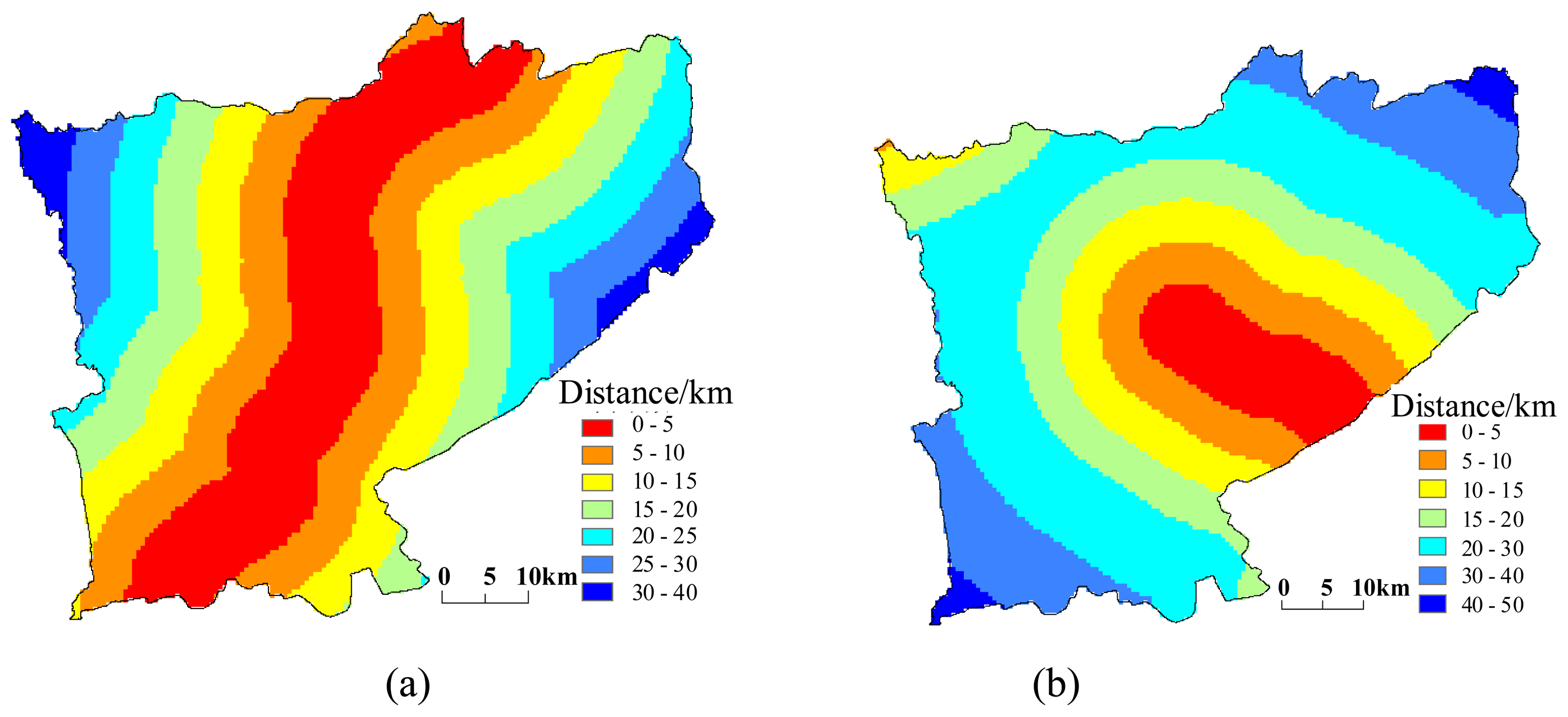
- Proximity variablesProximity variables including the distance from each pixel to the nearest provincial capital or highway, provincial road and county road are incorporated into surface to measure the impacts of the infrastructure facility on the dynamics of land systems. GIS software is used to calculate the proximity variables, based on the geographical database, including the road network and the location information of major cities around the case study area. Figure 4 shows the spatial variability of the distance of each pixel to the national expressway and the nearest provincial capitals.
- 4)
- Social and economic variablesSocial and economic variables, population density and gross domestic product (GDP) originally aggregated at the township level, are also spatially interpolated into the surface data. The historical data on the population and GDP are collected based on the household survey and field trip. The trends for the population growth and GDP expansion are projected based on the regional long-term planning of Taips County.
4. Results
4.1 Estimations of the coefficients of the influencing factors
4.2 Scenarios
4.2.1 Baseline scenario
4.2.2 Economic priority scenario
4.2.3 Environmental priority scenario
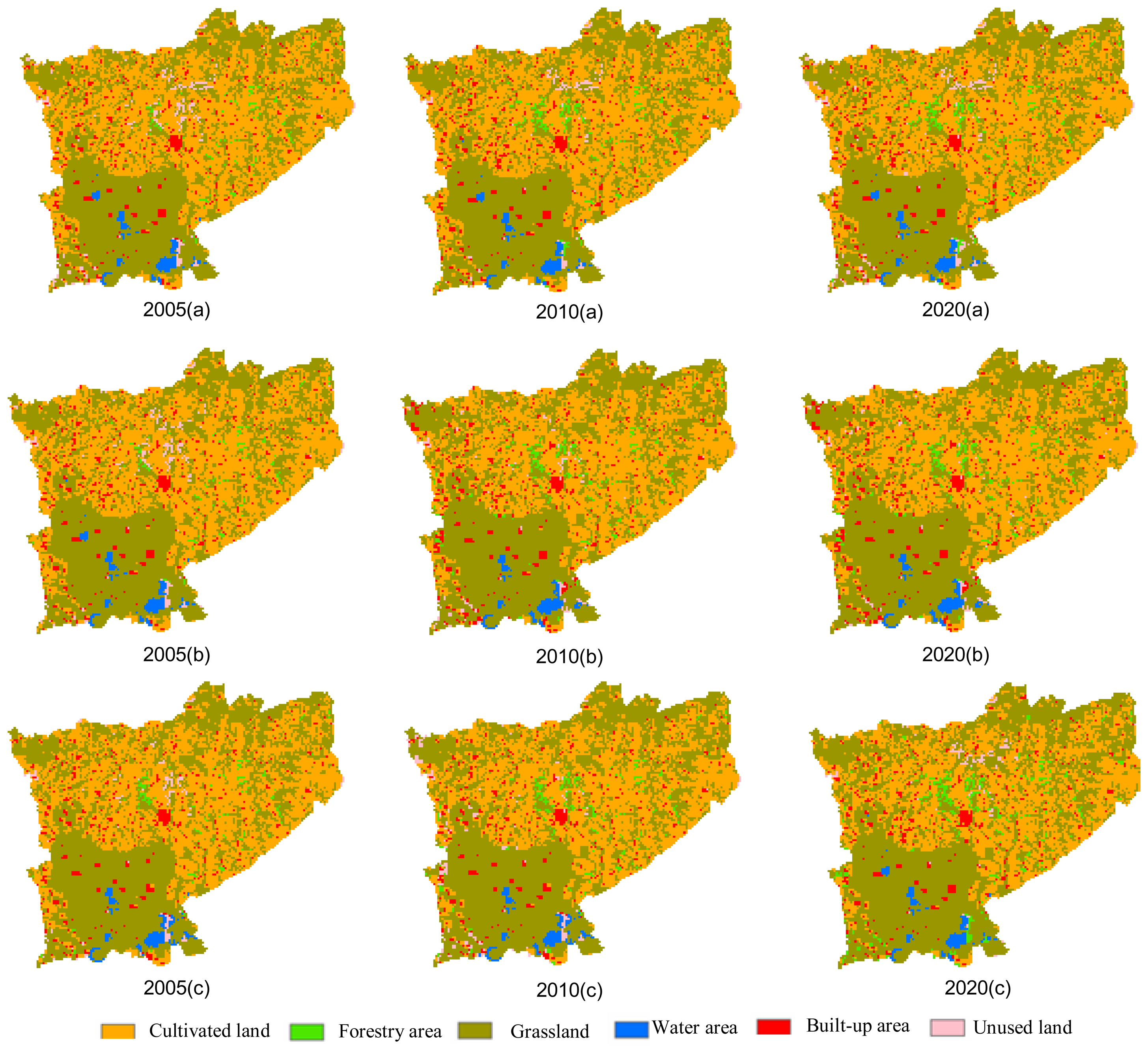
4.3 Dynamic simulation
5. Concluding remarks
Acknowledgments
References and Notes
- Turner, B.L., II; Skole, D.; Sanderson, S.; Fischer, G.; Fresco, L.; Leemans, R. Land-Use and Land-Cover Change.; Science/Research Plan: Stockholm and Geneva, 1995. [Google Scholar]
- Veldkamp, A.; Fresco., L.O. Exploring land use scenarios, an alternative approach based on actual land use. Agric. Syst. 1997, 55, 1–17. [Google Scholar]
- Global Land Project. Science Plan and Implementation Strategy; GLP: Stockholm, 2005; p. 64. [Google Scholar]
- Verburg, P.H.; Veldkamp, A. Introduction to the special issue on spatial modeling to explore land use dynamics. Int. J. Geog. Info. Sci. 2005, 19, 99–102. [Google Scholar]
- Verburg, P.H.; de Konig, G.H.J.; Kok, K.; Veldkamp, A.; Bouma, J. A spatial explicit allocation procedure for modeling the pattern of land use change based upon actual land use. Ecol. Model. 1999, 116, 45–61. [Google Scholar]
- Agarwal, C.; Green, G.M.; Grove, J.M.; Evans, T.P.; Schweik, C.M. A review and assessment of land-use change models: dynamics of space, time, and human choice.; USDA Forest Service PA: USA, 2002; p. 61. [Google Scholar]
- Kok, K.; Patel, M.; Rothman, D.S.; Quaranta, G. Multi-scale narratives from an IA perspective: Part II. Participatory local scenario development. Futures 2006, 38, 285–311. [Google Scholar]
- Verburg, P.H.; Rounsevell, M.D.A.; Veldkamp, A. Scenario-based studies of future land use in Europe. Agric. Ecosyst. Environ. 2006, 114, 1–6. [Google Scholar]
- Veldkamp, A.; Fresco., L.O. CLUE: a conceptual model to study the conversion of land use and its effects. Ecol. Model. 1996, 85, 253–270. [Google Scholar]
- Ligtenberg, A.; Bregt, A.K.; Lammeren, R.V. Multi-actor-based land use modeling: spatial planning using agents. Landscape Urban Plan. 2001, 56, 21–33. [Google Scholar]
- Bah, A.; Toure., I.; Le Page, C.; Ickowicz, A.; Diop, A.T. An agent-based model to understand the multiple uses of land and resources around drillings in Sahel. Math. Comp. Model. 2006, 44, 513–534. [Google Scholar]
- Dietzel, C.; Clarke, K. The effect of disaggregating land use categories in cellular automata during model calibration and forecasting. Comp. Environ. Urban Syst. 2006, 30, 78–101. [Google Scholar]
- Kok, K.; Verburg, P.H.; Veldkamp, T. Integrated Assessment of the land system: The future of land use. Land Use Policy 2007, 24, 517–520. [Google Scholar]
- Batty, M.; Xie, Y.; Sun, Z. Modeling urban dynamics through GIS-based cellular automata. Comp. Environ. Urban Syst. 1999, 23, 205–233. [Google Scholar]
- Castella, J.C.; Verburg, P.H. Combination of process-oriented and pattern-oriented models of land-use change in a mountain area of Vietnam. Ecol. Model. 2007, 202, 410–420. [Google Scholar]
- Chen, Y.; Verburg, P.H.; Xu, B. Spatial modeling of land use and its effects in China. Prog. Geograph. 2000, 19, 116–127. [Google Scholar]
- Verburg, P.H.; Soepboer, W.; Veldkamp, A.; Limpiada, R.; Espaldon, V. Modeling the spatial dynamics of regional land use: the CLUE-S model. Environ. Manag. 2002, 30, 391–405. [Google Scholar]
- Yue, T.X.; Wang, Y.A.; Liu, J.Y.; Chen, S.P.; Qiu, D.S.; Deng, X.Z.; Liu, M.L.; Tian, Y.Z.; Su, B.P. Surface modeling of human population distribution in China. Ecol. Model. 2005, 181, 461–478. [Google Scholar]
- Doll, C.N.H.; Muller, J.P.; Morley, J.G. Mapping regional economic activity from night-time light satellite imagery. Ecol. Econ. 2006, 57, 75–92. [Google Scholar]
- Price, D.T.; McKenney, D.W.; Nalder, I.A.; Hutchinson, M.F.; Kesteven, J.L. A comparison of two statistical methods for spatial interpolation of Canadian monthly mean climate data. Agric. For. Meteorol. 2000, 101, 81–94. [Google Scholar]
- Jeffrey, S.J.; Carter, J.O.; Moodie, K.B.; Beswick, A.R. Using spatial interpolation to construct a comprehensive archive of Australian climate data. Environ. Model. Soft. 2001, 16, 309–330. [Google Scholar]
- Hutchinson, M.F. Stochastic space-time weather models from ground-based data. Agric. For. Meteorol. 1995, 73, 237–264. [Google Scholar]


| Code | Land use | Description |
|---|---|---|
| 0 | Cultivated land | Original data include both paddy and non-irrigated uplands. |
| 1 | Forestry area | Natural or planted forests with canopy covers greater than 30%; land covered by trees less than 2 m high, with a canopy cover greater than 40%; land covered by trees with canopy cover between 10 to 30% and land used for tea-gardens, orchards and nurseries. |
| 2 | Grassland | Lands covered by herbaceous plants with coverage greater than 5% and land mixed rangeland with the coverage of shrub canopies less than 10%. |
| 3 | Water area | Land covered by natural water bodies or land with facilities for irrigation and water reservation, including rivers, canals, lakes, permanent glaciers, beaches and shorelines, and bottomland. |
| 4 | Built-up area | Land used for urban and rural settlements, industry and transportation. |
| 5 | Unused land | All other lands. |
| Influencing factors | Definitions (units between parentheses) |
|---|---|
| Geophysical variables | |
| Terrain | 0: Hills |
| 1: Plain | |
| 2: Mesa | |
| 3: Plateau | |
| Soil pH value | pH values of soil. The higher the value is, the lower the acidity of the soil. |
| Depth of soil | Depth of top soil (cm) |
| Elevation | Digital Elevation Model (m) |
| Slope | Terrain slope derived from DEM (0.01 degrees) |
| Climatic variables | |
| Air temperature | Mean annual temperature (0.1 °C) |
| Cumulated temperature (≥0 degrees Centigrade) | Annually cumulated temperature of daily mean air temperature above 0 °C (0.1 °C) |
| Cumulated temperature (≥10 degrees Centigrade) | Annually cumulated temperature of daily mean air temperature above 10 °C (0.1 °C) |
| Sun-shining hours | Sunshine hours rectifying the spatial variability of solar radiation |
| Proximity variables | |
| Distance to province capital | Geometric distance to nearest province capital |
| Distance to the highway | Distance to the nearest highway (km) |
| Distance to the expressway | Distance to the nearest expressway (km) |
| Socio-economic variables | |
| Population density | Interpolated population density (persons/km2) based on the Surface Modeling of Population Distribution [18]. |
| GDP | Interpolated values of Gross Domestic Product (GDP) (10000 yuan/km2) based on the spatially explicated analyses on the relationship between economic growth level and factors that might affect economic growth [19] |
| Influencing factors | Cultivated land | Forestry area | Grassland | Water area | Built-up areas | Unused land |
|---|---|---|---|---|---|---|
| Terrain: plain (0,1) | 0.018 (0.021) | 0.198 (2.44) | 0.057 (2.66) | 1.009 (0.39) | 0.233 (3.26) | 1.638 (4.26) |
| Terrain: mesa (0, 1) | -1.560 (-19.00) | 0.394 (1.71) | -2.527 (-57.22) | 6.510 (2.52) | 0.343 (2.09) | 5.128 (13.28) |
| Terrain plateau (0, 1) | 0.199 (9.73) | 0.416 (5.18) | -0.390 (-18.28) | 4.537 (1.76) | 0.738 (10.78) | 3.484 (9.10) |
| Soil pH value | -3.22 (-16.00) | 1.307 (1.68) | 0.831 (3.92) | 38.155 (7.18) | 0.912 (1.59) | -1.293 (-1.14) |
| Soil depth | -0.265 (-7.27) | -3.587 (-14.42) | 0.323 (8.47) | -4.294 (-14.00) | -1.349 (-12.43) | -0.187 (-1.17) |
| Elevation | -0.001 (-8.64) | 0.006 (8.52) | 0.001 (2.92) | -0.023 (-25.25) | -0.003 (-9.22) | 0.017 (35.08) |
| Slope | 0.001 (15.14) | -0.001 (-0.76) | -0.001 (-6.82) | -0.014 (-23.46) | -0.002 (-11.44) | -0.002 (-7.42) |
| Air temperature | 2.039 (16.73) | 7.404 (12.14) | -1.771 (-14.07) | 12.609 (21.27) | 2.421 (6.90) | -0.606 (-1.42) |
| Rainfall | -0.008 (-6.73) | -0.103 (-14.54) | 0.007 (5.51) | 0.029 (3.68) | -0.024 (-6.62) | -0.029 (-6.66) |
| Cumulative temperature(>=0) | -0.003 (-3.13) | -0.013 (-3.11) | 0.009 (10.00) | -0.114 (-12.35) | -0.012 (-5.05) | -0.010 (-3.45) |
| Cumulative temperature(>=10) | 0.001 (9.58) | -0.001 (-1.65) | 0.001 (8.37) | 0.015 (1.32) | 0.001 (2.53) | -0.015 (-32.01) |
| Sunshine hours | 0.397 (21.91) | 0.481 (5.84) | -0.377 (-20.53) | 1.299 (13.07) | 0.643 (13.89) | -1.138 (-20.77) |
| Distance to provincial capital | 0.006 (10.42) | 0.047 (16.50) | 0.001 (1.77) | -0.026 (-6.23) | 0.013 (8.34) | -0.027 (-13.66) |
| Distance to highway | -0.021 (-12.62) | -0.119 (-14.25) | 0.031 (17.79) | -0.088 (-8.59) | -0.056 (-12.81) | 0.050 (8.27) |
| Distance to the expressway | 0.016 (24.8) | 0.014 (3.80) | -0.002 (-3.31) | -0.046 (-10.36) | -0.013 (-7.03) | -0.043 (-16.25) |
| Population density | 0.034 (23.52) | -0.01 (-3.78) | -0.041 (-252.94) | -0.025 (-20.43) | -0.002 (-14.17) | -0.026 (-37.23) |
| GDP | -0.089 (219.49) | 0.011 (10.34) | 0.090 (212.67) | -0.191 -36.09 | 0.040 (94.63) | -0.040 (-14.62) |
| Constant | -62.17 (-12.39) | -28.142 (-1.27) | 53.852 (10.47) | -303.115 (-5.99) | -109.035 (-8.44) | 331.938 (17.82) |
| Observation numbers | 345895 | 345895 | 345895 | 345895 | 345895 | 345895 |
| Pseudo R2 | 0.237 | 0.1146 | 0.2516 | 0.4690 | 0.2893 | 0.2859 |
© 2008 by MDPI Reproduction is permitted for noncommercial purposes.
Share and Cite
Deng, X.; Su, H.; Zhan, J. Integration of Multiple Data Sources to Simulate the Dynamics of Land Systems. Sensors 2008, 8, 620-634. https://doi.org/10.3390/s8020620
Deng X, Su H, Zhan J. Integration of Multiple Data Sources to Simulate the Dynamics of Land Systems. Sensors. 2008; 8(2):620-634. https://doi.org/10.3390/s8020620
Chicago/Turabian StyleDeng, Xiangzheng, Hongbo Su, and Jinyan Zhan. 2008. "Integration of Multiple Data Sources to Simulate the Dynamics of Land Systems" Sensors 8, no. 2: 620-634. https://doi.org/10.3390/s8020620
APA StyleDeng, X., Su, H., & Zhan, J. (2008). Integration of Multiple Data Sources to Simulate the Dynamics of Land Systems. Sensors, 8(2), 620-634. https://doi.org/10.3390/s8020620