Robust Forecasting for Energy Efficiency of Wireless Multimedia Sensor Networks

Abstract

An important criterion of wireless sensor network is the energy efficiency in specified applications. In this wireless multimedia sensor network, the observations are derived from acoustic sensors. Focused on the energy problem of target tracking, this paper proposes a robust forecasting method to enhance the energy efficiency of wireless multimedia sensor networks. Target motion information is acquired by acoustic sensor nodes while a distributed network with honeycomb configuration is constructed. Thereby, target localization is performed by multiple sensor nodes collaboratively through acoustic signal processing. A novel method, combining autoregressive moving average (ARMA) model and radial basis function networks (RBFNs), is exploited to perform robust target position forecasting during target tracking. Then sensor nodes around the target are awakened according to the forecasted target position. With committee decision of sensor nodes, target localization is performed in a distributed manner and the uncertainty of detection is reduced. Moreover, a sensor-to-observer routing approach of the honeycomb mesh network is investigated to solve the data reporting considering the residual energy of sensor nodes. Target localization and forecasting are implemented in experiments. Meanwhile, sensor node awakening and dynamic routing are evaluated. Experimental results verify that energy efficiency of wireless multimedia sensor network is enhanced by the proposed target tracking method.

1. Introduction

Wireless sensor networks (WSNs) consist of a large number of intelligent sensor nodes integrated into the environment, accomplishing complicated tasks, such as target tracking and environment surveillance. Sensing, processing and communication capabilities are enabled on each sensor node. WSNs are attractive because they can be deployed in nearly any kind of environment without wired connections. More recently, the availability of inexpensive hardware (such as microphones) that are able to ubiquitously capture multimedia content from the environment has fostered the development of wireless multimedia sensor networks (WMSNs) [1,2]. WMSN is equipped by wirelessly interconnected devices that allow retrieving multimedia data, such as video and audio streams. As sensor nodes usually work in unsupervised area, the battery can not be recharged or replaced. To prolong the lifetime of WMSN, energy efficiency becomes a crucial issue.

The target tracking application of WMSN is investigated, where acoustic sensors are adopted to localize the target. Each sensor node can acquire acoustic signals from the target. In centralized networks, there are usually sink nodes for global processing and control. To enhance the resilience of WMSN against sensor node failures or congestion conditions around the sink node, self-organizing and distributed decision of sensor nodes are useful approaches [3]. Considering the target tracking performance, a distributed architecture of WMSN should be exploited to avoid large communication overheads in the centralized approach. For the sensor nodes, it is assumed that the low-power sleep mode is supported by their operation system, i.e., sensor node can switch between active mode and sleep mode. As described in [4], the power consumption of sleep mode is usually several orders of magnitude less than that of active mode. Energy saving can be achieved by sending sensor node to sleep as much as possible when there is no sensing, processing or communication task. To enhance the energy efficiency and the detection accuracy of WMSN, the sleep coordination and collaborative localization of sensor nodes can be performed with the prior target motion information derived from target tracking procedure. Therefore, target position forecasting is necessary during target tracking.

As the state model of target motion is nonlinear, so target tracking is usually treated as nonlinear estimation problems [5]. The classical method is extending the standard Kalman filter to nonlinear system by local linearizing all nonlinear models around certain points, which is so called Extended Kalman filter (EKF) [6]. In practical, the target may have high maneuvers. Some algorithms have been proposed for maneuvering target tracking, such as unscented Kalman filter (UKF) [7] and unscented particle filter (UPF) [8]. However, these algorithms are computation-expensive under the constraints of limited processing capability. An algorithm with low complexity is desirable for target tracking in WMSN, especially for the distributed computation on general sensor nodes. Thus, autoregressive moving average (ARMA) model [9] can be taken into account for target tracking. The forecasting efficiency of ARMA model has been justified in many applications, such as power system [10]. However, the high uncertainty of maneuver which brings estimation error into the forecasting process should be handled in this case. Otherwise, it would degrade the performance of target tracking, or even miss the target (when the target detection is directed by the forecasting results). Therefore, the estimation error of model should be compensated, where artificial neural networks can be considered. As radial basis function networks (RBFNs) [11] have excellent performance on computation precision and convergence speed, it can be employed here. As mentioned earlier, the forecasted target position can be utilized to schedule the operation mode of sensor nodes in order to save energy. Also, more reasonable decision can be made with the forecasting results when multiple sensor nodes localize the target collaboratively. In addition, the data delivery and query/response process should be exploited under the distributed architecture of WMSN.

Considering target tracking performance and the energy efficiency of WMSN, an energy-efficient target tracking method is proposed with robust target forecasting. Firstly, a totally distributed architecture is proposed, i.e. without the requirement of a sink node. The regular geometric structure of WMSN is considered to obtain stable coverage and connectivity. Especially, the honeycomb configuration is utilized to provide the most efficient coverage with specified sensor node number. Then, a novel algorithm is proposed for target position forecasting, which is so-called ARMA-RBF. It is a combination of ARMA model and RBFN. According to the historical target positions, the parameters of ARMA model are estimated dynamically and the RBFN is trained to compensate the estimation error. Meanwhile, the data delivery approach is presented to support the distributed processing of sensor nodes. With the forecasting results, sensor nodes are awakened to active mode for the future detection task. As multiple sensor nodes can acquire the acoustic signals, the target is localized via committee decision [12]. With energy attenuation model of acoustic signal, the committee decision is realized by RBFN, which is trained in advance to depict the mapping from related signal energy feature to target position. Furthermore, the sensor-to-observer routing scheme for reporting the target position is discussed in the network with honeycomb configuration. Experiments analysis is presented to justify the efficiency of the proposed target tracking method while the localization accuracy improvement and energy saving of WMSN are illustrated.

The rest of this paper is organized as follows. Section 2 presents the related work of this research. Section 3 defines the acoustic signal sensing model and distributed honeycomb configuration in WMSN. In particular, the energy consumption model is given for the target tracking application. In Section 4, the energy-efficient target tracking method is described in detail. The future target position forecasted by ARMA-RBF is adopted in the sleep mode scheduling and committee decision. Beside, the sensor-to-observer routing is presented for target position reporting. The experiments results are presented in Section 5, where the energy-efficient target tracking method with robust target forecasting is applied in WMSN. We conclude the paper in Section 6.

2. Related Work

Energy efficiency has drawn a lot of attention from various aspects of WSN research, such as hardware layer, media access control (MAC) layer, network layer, application layer, and so on [13]. Here, the target tracking application is discussed and we focus on the energy optimization on the network and application layers. Still, the multiple operation modes of sensor node are considered for power management. That is because the modules of sensor node can be well controlled by their operation system now [14].

First of all, the deployment of WSN is discussed. The regular deployment is considered in this paper. To deploy the sensors based on a regular geometric topology, a precision weapon can be used to place the sensor nodes [15]. Although it is costly to deploy a regular structure of WSN, simpler and more efficient methods are readily available and a regular structure may benefit the specified application.

Furthermore, the WSN we discuss can capture and process multimedia data, which is so-called WMSN. Video or audio sensors can be used to enhance and complement existing surveillance systems against crime and terrorist attacks [1]. Here, the acoustic sensors are adopted to localize the target. In [16], an environmental monitoring system is provided to record animal behaviors for a long period of time. The shooter localization system collects the time stamps of the acoustic detection from different nodes within the network to localize the positions of the snipers [17]. The Line-in-the-Sand project focuses on target tracking and classification [18]. Localization problems with acoustic signal are overviewed in [19]. It shows localization is primarily achieved by two approaches, i.e. by estimate of time delay of arrival (TDOA) or estimate of energy attenuation. Each algorithm has its own advantages and disadvantages [20]. In [21], energy based localization using acoustic signal in WSN is presented. We adopt the model of acoustic energy attenuation for target localization, because it is relatively easy to establish and less influenced by environmental changes.

The target tracking application is considered under the honeycomb configuration. To solve the energy efficiency problem in application layer, some energy-efficient approaches have been proposed [22]. In [23], a tree-based algorithm is proposed to facilitate collaborative tracking of moving targets. Authors of [24] propose a particle filtering (PF) style tracking algorithm using binary sensors, which can detect whether an object is approaching or not. Besides, a distributed tracking system based on extended Kalman filter (KF) techniques is implemented in [25]. Based on an information-driven approach, a tracking system is built in [26] with distributed Bayesian estimation, given previous estimation and new sensor inputs. Compared to the limited processing capability, the tracking algorithms (such as KF and PF) may be computational-expensive for sensor nodes in a distributed WSN. As target state can be easily modeled by ARMA process, some researches have taken ARMA model into account for target tracking [27]. An ARMA model based scheme is proposed for tracking maneuvering targets in the Cartesian coordinate system.

Considering the maneuver of target, the algorithm combining ARMA model and artificial neural networks is discussed. In the application of short-term load forecasting (STLF), a combinational approach of BP networks and ARMA model is proposed in [28]. In this paper, error compensation of ARMA model is performed by RBFN. That is because RBFNs not only have better computation precision than back propagation (BP) networks but also converge faster than BP networks [29]. In addition, we introduce committee decision into the target localization.

At the network layer, methods have been proposed to balance power through the distribution of messages among various paths from source to destination or to use efficient cache schemes to balance the energy cost between data query and dissemination. In [30], data aggregation techniques are used to reduce energy consumption by aggregating multiple reports about the same event. However, the routing scheme should be designed according to target tracking application, especially in the distributed WSN. Here, data delivery approach and sensor-to-observer routing are proposed based on the honeycomb configuration.

In particular, an energy management protocol for target tracking is proposed in [31]. In this work, the sensor nodes far away from the target are allowed to sleep. However, not enough effort has been made on extracting the target motion information for sleep scheduling.

The difference of our work from aforementioned approaches mainly includes the following three aspects: (1) the WMSN is organized in a distributed manner, where the honeycomb configuration is discussed; (2) the energy efficiency of WMSN benefits from the prior information of target motion, which is extracted by ARMA-RBF algorithm; (3) target localization with committee decision based on the acoustic energy attenuation model. Besides, data delivery approach and sensor-to-observer routing are exploited in this distributed WMSN with honeycomb configuration.

3. Preliminaries

We consider a scenario that WMSN is formed by stationary sensor nodes in two-dimension sensing field. Sensor nodes are equipped with acoustic sensors and work collaboratively for target tracking, where the vehicle target is discussed. In this section, acoustic signal sensing model is given first. Based on the sensing model of sensor nodes, a distributed honeycomb configuration will be defined for WMSN. Considering the energy efficiency of target tracking application, the energy consumption model of WMSN will be presented.

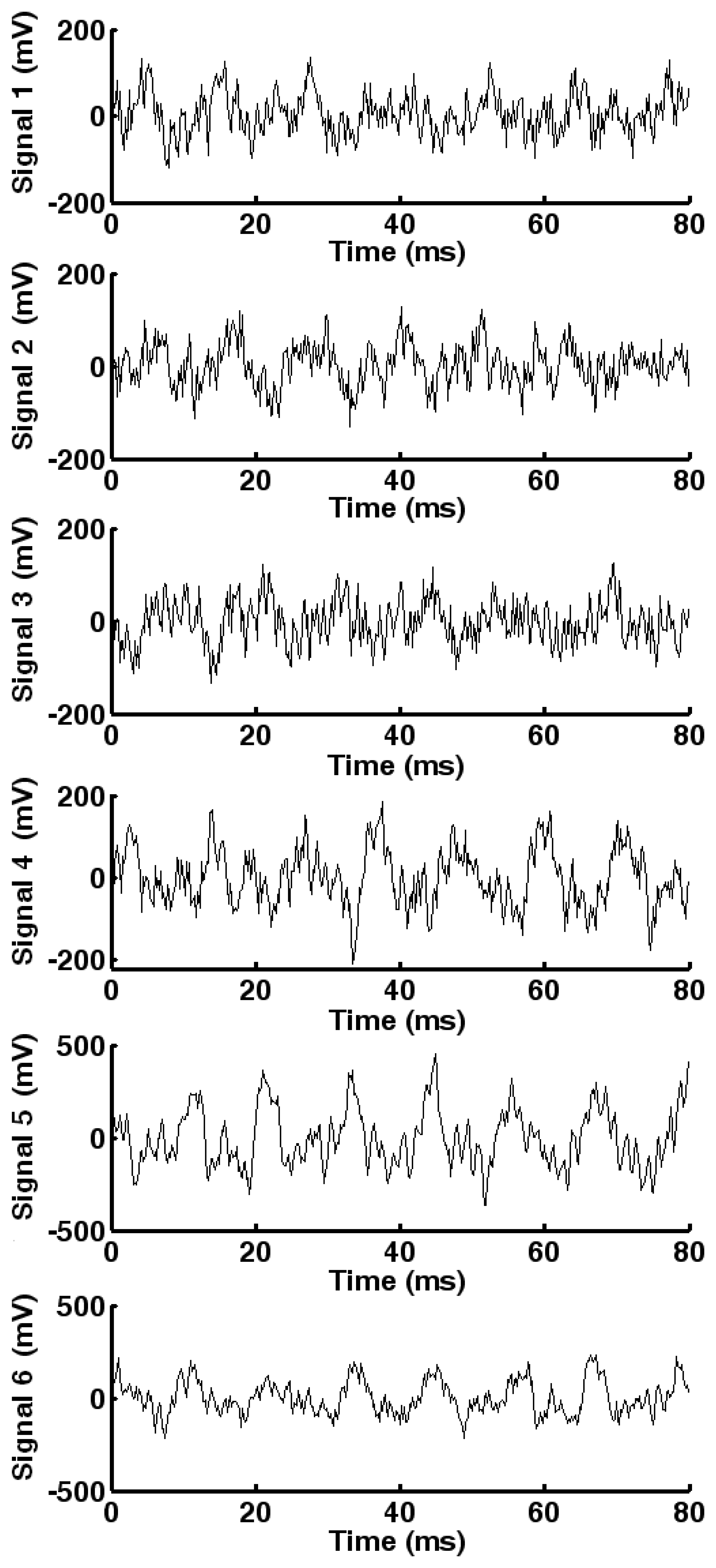
3.1. Acoustic Signal Sensing Model

With rapid improvements and miniaturization in hardware, a single sensor device can be equipped with audio information collection modules [1]. Here, each sensor node is equipped with one microphone. For the vehicle target, the acoustic signal emitted from the engine can be sensed by the sensor nodes.

The way that acoustic signal propagates with the distance from the source is dependent on the size and shape of the source, the surrounding environment, prevailing air currents and the frequencies of the propagating acoustic signal [32]. Other factors that may affect sound propagation may include wind direction, strength of wind, vegetation such as forest and other obstructions. To simplify the problem, it is assumed that the acoustic signal propagation in the free air and the acoustic source is treated as an omni-directional point.

For a given target, the acoustic signal propagation is discussed in the two-dimension sensing field. Suppose that the source position of acoustic signal (target position) is denoted by p_s = [x_s, y_s]^T. The acoustic signal at p_s is denoted by u_s(t). Two-dimension propagation of the acoustic signal is mathematically represented by [19,20]. The acoustic signal at the position p_d=[x_d, y_d]^T can be calculated as:

$$u_d^{\prime }(t)=\frac{1}{4\pi \Vert p_s-p_d\Vert }{u}_s(t-t_{sd})$$

(1)

where ‖ · ‖ represents the vector 2-norm, which is defined as:

$$\Vert {[x,y]}^T\Vert =\sqrt{x^2+y^2}$$

(2)

t_sd denotes the propagation time of acoustic signal from position p_s to p_d, which is calculated as:

$$t_{sd}=\frac{\Vert p_s-p_d\Vert }{c}$$

(3)

where c is propagation velocity of acoustic signal. It can be taken as a constant in this case.

For the sensor node located at position p_d, the acoustic signal sensed by this sensor node is represented as:

$$u_d(t)=\frac{{\alpha }_d}{4\pi \Vert p_s-p_d\Vert }{u}_s(t-t_{sd})+n_d(t)$$

(4)

where the gain of microphone is denoted by α_d. n_d(t) is the zero-mean additive white Gaussian noise (AWGN) from the environment, which is assumed to be uncorrelated with the source acoustic signal.

Equation (4) is a comprehensive description of the propagating characteristics of acoustic signals. Information of the acoustic source can be inferred from this equation. Specifically the problem is to estimate p_s from the acoustic signal u_d(t) sensed by the sensor node.

When an acoustic signal is propagating, it essentially propagating energy emitted from the source. For the acoustic sensed by the sensor node, the expectation of energy is denoted by $E[u_d^2(t)]$. E[·] means the expected value. According to Equation (4), we have:

$$\begin{array}{l}E[u_d^2(t)]=\frac{{\alpha }_d^2}{16{\pi }^2{\Vert p_s-p_d\Vert }^2}E[u_s^2(t-t_{sd})]+E[n_d^2(t)]\\ =\frac{{\alpha }_d^2}{16{\pi }^2{\Vert p_s-p_d\Vert }^2}E[u_s^2(t)]+E[n_d^2(t)]\end{array}$$

(5)

where $E[u_s^2(t)]$ and $E[n_d^2(t)]$ are the expectation of energy for the source acoustic signal and noise, respectively. Here, the expectation of energy is calculated by averaging over a time window:

$$T_w=\frac{M_w}{f_s}$$

(6)

where M_w is the number of sample points we used for averaging the energy, and f_s is the sampling frequency of microphone.

Here, the target to be discussed is a truck. Thus, the term $E[n_d^2(t)]$ in Equation (5) can be ignored, compared to the energy of acoustic signal from truck engine. Then the acoustic energy attenuation model can be described as:

$$\frac{E[u_d^2(t)]}{E[u_s^2(t)]}=\frac{{\alpha }_d^2}{16{\pi }^2{\Vert p_s-p_d\Vert }^2}$$

(7)

u_s(t), p_d and p_s are unknown here, so the target position can be estimated by combining the observations of multiple sensor nodes. Therefore, the target localization approach will be exploited with the known energy of acoustic signal.

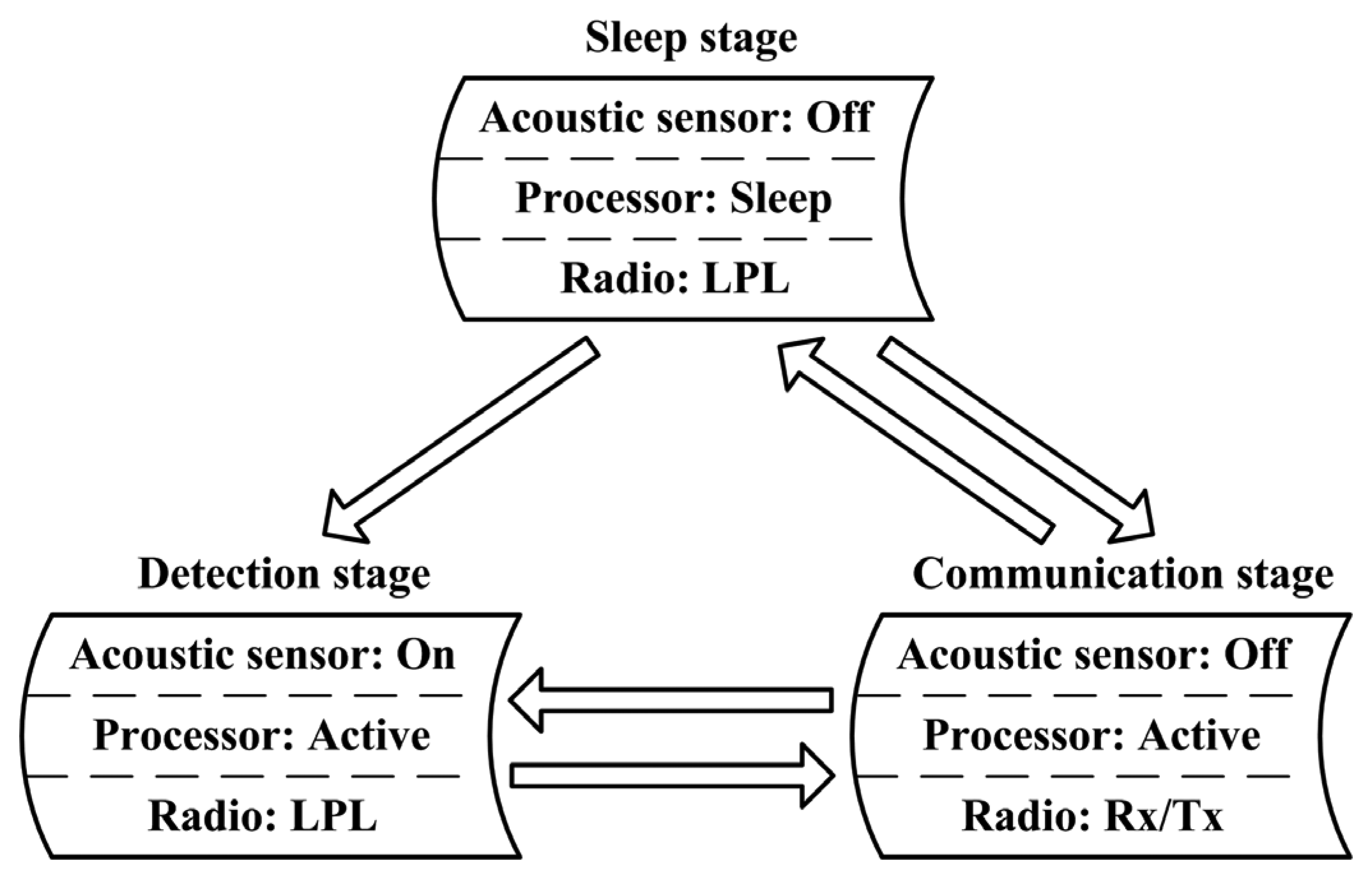
3.2. Energy Consumption Model

In this target tracking application, each sensor node is mainly composed of three components: acoustic sensor, processor and radio. For the scalability of energy consumption in WSN, all the components of sensor node are supposed to be controlled by an operation system, such as microOperating System (μOS) [14]. Shutting down or turning on any component is enabled by device drivers in the specified application of WMSN. Thus, sensor nodes can go into sleep to prolong the lifetime. Accordingly, reasonable awakening approach should be exploited with the target motion information.

Firstly, the characteristics of the acoustic sensor and processor components are presented in

Table 1. Power consumption and startup time of acoustic sensor and processor in different modes.

Component	Acoustic sensor		Processor
Operation mode	Off	On	Sleep	Active
Power consumption (mW)	0.003	1.73	0.03	24
Startup Time (ms)	1		0.2

. The acoustic sensor component has “off” and “on” operation modes while the processor component has “sleep” and “active” operation modes. The lower power modes imply great potential for energy saving. Besides, the startup time means the transition latency between the operation modes.

Then, the characteristics of radio component will be discussed. Generally, the radio component has two modes: “LPL” and “Rx/Tx”. Here, LPL is an acronym for low-power listening. In this mode, the radio can listen to the media with low power consumption, 0.411 mW. Furthermore, the radio can perform data reception and transmission in the “Rx/Tx” mode. The transition latency between the two modes is 2.5 ms. Power consumption of “Rx/Tx” mode includes two parts, which can be presented as:

$$P_{Tx/Rx}=P_{Rx}+P_{Tx}$$

(8)

where P_RX and P_TX are the power consumption for data reception and transmission, respectively. P_RX is regarded as a constant, 24 mW, while P_TX is dependent on the transmission range. It is assumed that the sensor nodes are placed in the two-dimension field without obstacle. When sensor node i transmits data to sensor node j, the power received by sensor node j has the following relation with the power transmitted by sensor i according to the Friis free space propagation model [12]:

$$P_j=P_i\frac{G_t{G}_r{\lambda }^2}{{(4\pi )}^2{d}_{i,j}^2\beta }$$

(9)

where G_t is the gain of transmitter, G_r is the gain of receiver, λ is the radio wavelength, and β is the system loss factor. The physical distance d_i,j between sensor node i and j is computed from the spatial locations. With the receiving power threshold P_th, each sensor node should have the transmission power P_Tx to cover the communication range R_c:

$$P_{Tx}=P_{th}\frac{{(4\pi )}^2{R}_c^2\beta }{G_t{G}_r{\lambda }^2}$$

(10)

Here, the transition latency and power consumption are typical values referred to [33].

According to the different modes of components, three stages are defined for each sensor node during target tracking: sleep stage, detection stage and communication stage. As shown in Figure 1, the hardware configuration and transition order are given for these stages. Sensor nodes keep low energy consumption in the sleep stage. Only the radio component is set in “LPL” mode. It is assumed that sensor nodes in this stage can be awakened by the messages from other sensor nodes [33]. In the detection stage, the acoustic sensor and processor components are turned on while the radio component is turned off. Thus, the sensor node can acquire and process the acoustic signal. In addition, sensor nodes transfer data in the communication stage. Here, the radio component is set in “Rx/Tx” mode and the processor component is active. With the defined transition latency of components, the latency between the stages can be obtained following the transition order. As the component should be shut down or turned on one by one, the latency between the stages is given in

Table 2. Latency between sleep stage, detection stage and communication stage for each sensor node.

Latency (ms)		Destination stage
		Sleep	Detection	Communication
Original stage	Sleep	-	1.2	2.7
	Detection	-	-	3.5
	Communication	2.7	3.5	-

. The transition of these stages will be utilized to enhance the energy efficiency of target tracking.

For each sensor node, the total energy consumption at time instant t can be calculated as:

$$E_{\mathit{\text{total}}}(t)=\underset{\tau =0}{\overset{t}{\int }}P(\tau )d\tau$$

(11)

where P(τ) means the power consumption at time instant τ for this sensor node. Thus, the residual energy can be calculated as:

$$E_r(t)=E_0-E_{\mathit{\text{total}}}(t)$$

(12)

where E₀ denotes the initial energy of sensor node.

With this energy consumption model, the energy usage of WMSN can be scheduled properly.

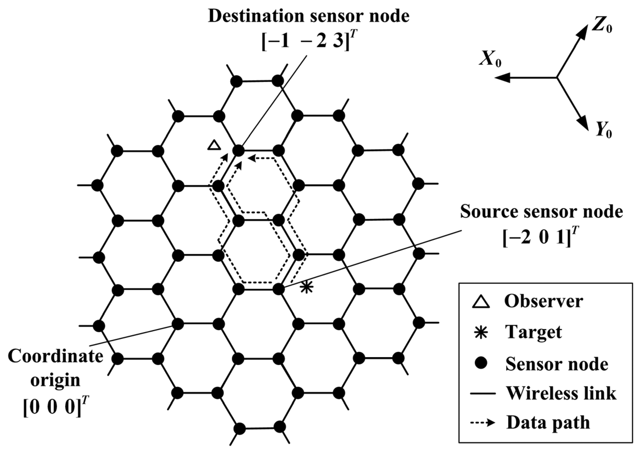
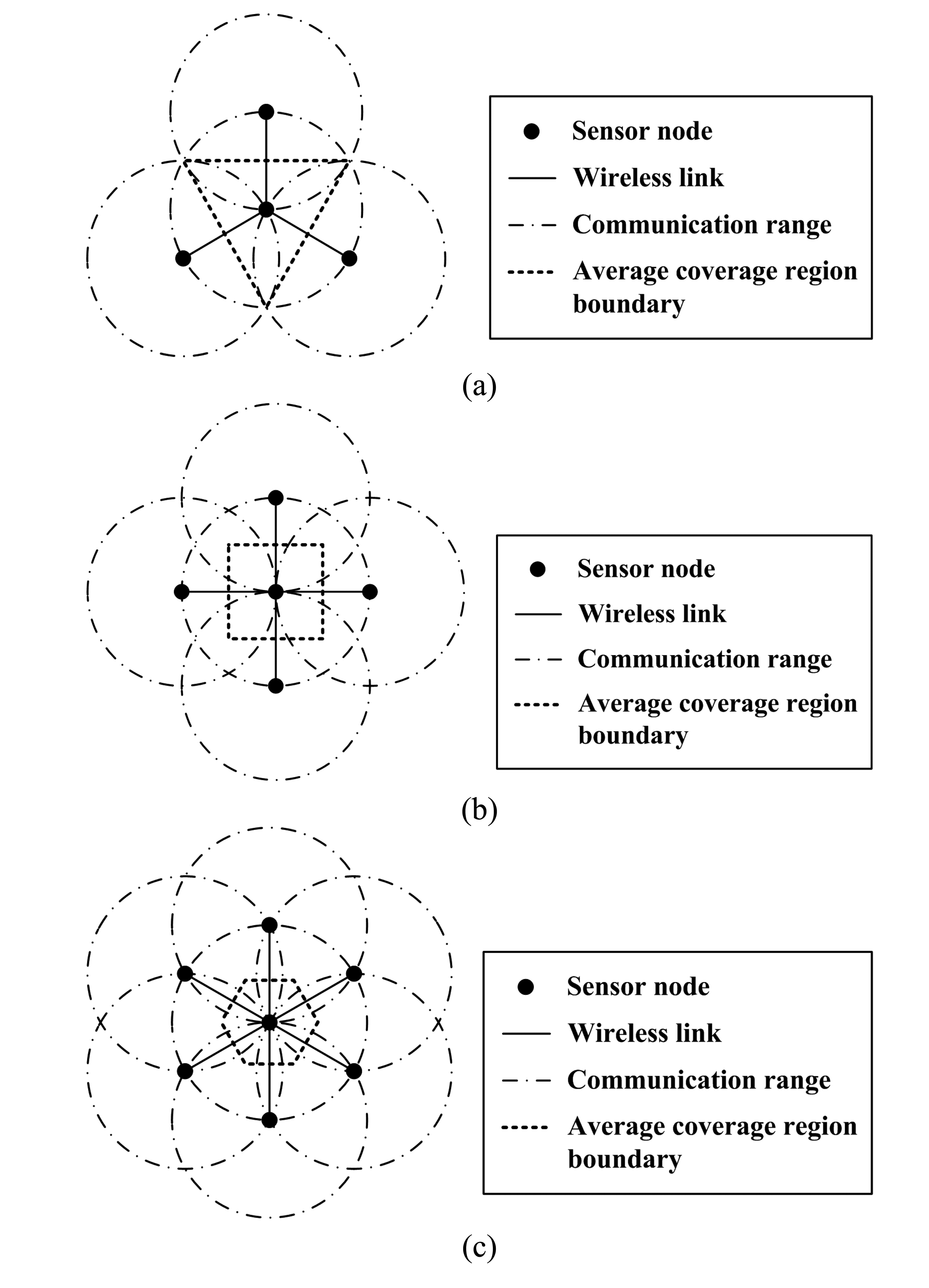
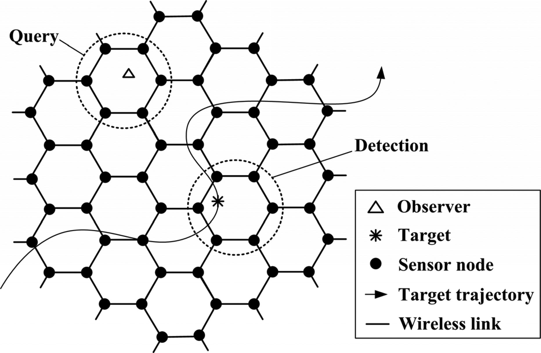
3.3. Distributed Honeycomb Configuration

For the target tracking application, a distributed WMSN will be discussed to provide flexible and adaptive capability. The deployment of sensor nodes is designed in advance. For the stable detection performance of target tracking, the regular deployment of sensor nodes is considered.

As described in Section 3.1, the microphone sensors are used to localize the target. For this kind of passive detection sensors, the sensing range is not only determined by the sensitivity, but also strongly influenced by the intensity of acoustic signal produced by the target. In [34], it has shown that the effective sensing range of microphone is about 100 m in the vehicle detection, that is, sensor nodes within a range of 100 m may have contribution to the vehicle localization. According to Section 3.2, the long distance communication will be prohibitively expensive for the energy-limited sensor nodes. To reduce communication energy consumption and form reliable links among sensor nodes, the communication range is limited. Referring to [35] and [36], the allowed communication range R_c of sensor node is at most 50 m. Compared to sensing coverage, the communication coverage should be mainly considered in WMSN.

As a functionality of WMSN, observers can query the target tracking result from any location of the sensing field through wireless equipments. Thus, the sensing field should be fully covered in the communication coverage problem. In this case, sensor nodes are regularly deployed. For each sensor node, the sensor nodes in the communication range are defined as its neighbors. Considering the coverage efficiency, the distance from the sensor node to any neighbor is a constant, which is equal to the communication range R_c. In the two-dimension field, sensor nodes can have 3, 4 or 6 neighbors to form a regular deployment. As shown in Figure 2, the coverage efficiency of different network structures is analyzed. Ignoring the coverage situation on the sensing field boundary, the coverage efficiency can be evaluated as:

$$CE=\frac{S_a}{\pi {R_c}^2}$$

(13)

where S_a is the average coverage area for each sensor node. In Figure 2, we can find that the average coverage area is $3\sqrt{3}{R_c}^2/4$, R_c² and $\sqrt{3}{R_c}^2/2$ for 3, 4 and 6-neighbor structures respectively. The 3-neighbor structure obtains the highest coverage efficiency (CE = 0.413).

The corresponding topology types for the 3, 4 and 6-neighbor structures are hexagon, square and triangle. The hexagon network has been justified in [37] to have the highest transmit probability, throughput, and effective transport capacity. Thus, the 3-neighbor structure is chosen for the network deployment. Thus, a specified sensing field can be covered by least sensor nodes.

According to the 3-neighbor structure, the location of sensor node can be determined by the network scale. As shown in Figure 3, a WMSN with honeycomb configuration is established for the target tracking application. There is no sink node and each sensor node can only communicate with its neighbors. Thereby, the sensor nodes work in a distributed manner to accomplish target tracking tasks. According to the above-mentioned definition, the 6 sensor nodes on the hexagon where the target located have the opportunity to acquire the acoustic information. Thus, collaborative target localization can be performed essentially. Also, the sensor node should be self-organized to report the target tracking results adaptively when there is any query from the observers.

With the introduced models, the localization accuracy and energy consumption problem will be addressed. Low-complexity and robust tracking algorithms will be exploited while the energy-efficient mode scheduling of sensor nodes will be provided. Also, application-oriented routing scheme will be discussed.

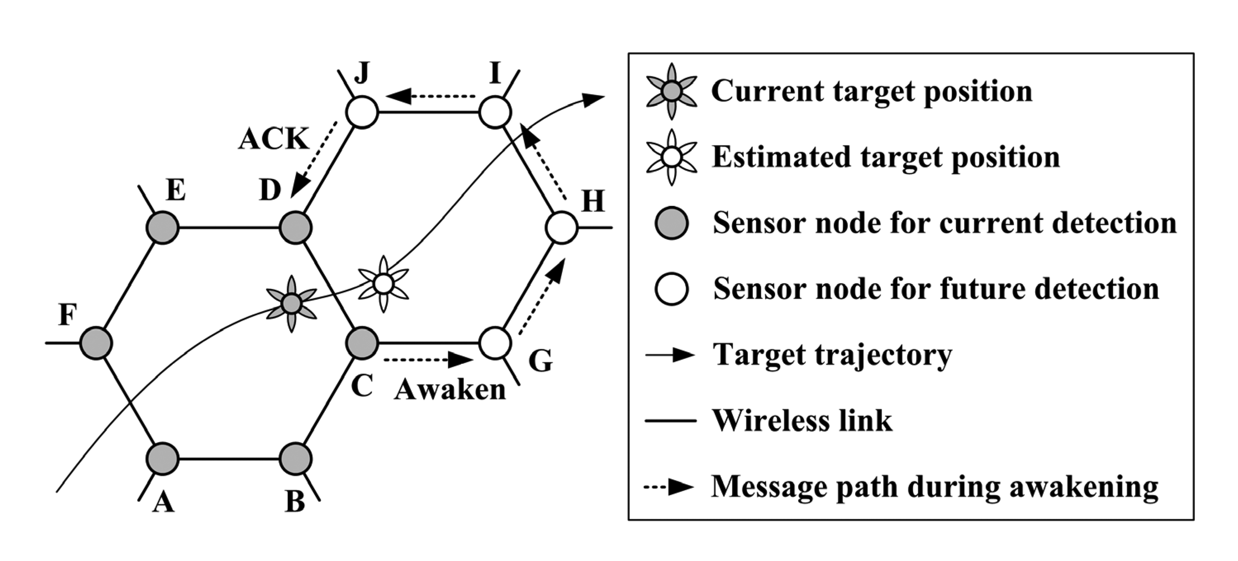
4. Energy-efficient Target Tracking Method

In this section, the energy-efficient target tracking method will be described in detail. With the defined network structure, the target tracking procedure is shown in Figure 4. In WMSN, target localization is performed with constant period T. For the k -th sensing period, the p historical target positions from (k−p+1)T to kT are utilized to forecast the target position at time instant (k+1)T. A novel algorithm, ARMA-RBF, is proposed to perform the target prediction.

With the estimated target prediction, the sensor node around the target will be awakened in advance for target localization while the other sensor node can keep in the sleep stage to save energy. To guarantee that the acquired acoustic signals are associated with the same time interval, time synchronization is implemented during sensor node awakening. As the target localization task is time-critical, RBFN is adopted to attain the current target position according to the acoustic signal sensing model. The committee decision is employed to fuse the results of different sensor node group. Besides, a sensor-to-observer routing scheme is introduced for response the data query from the observers.

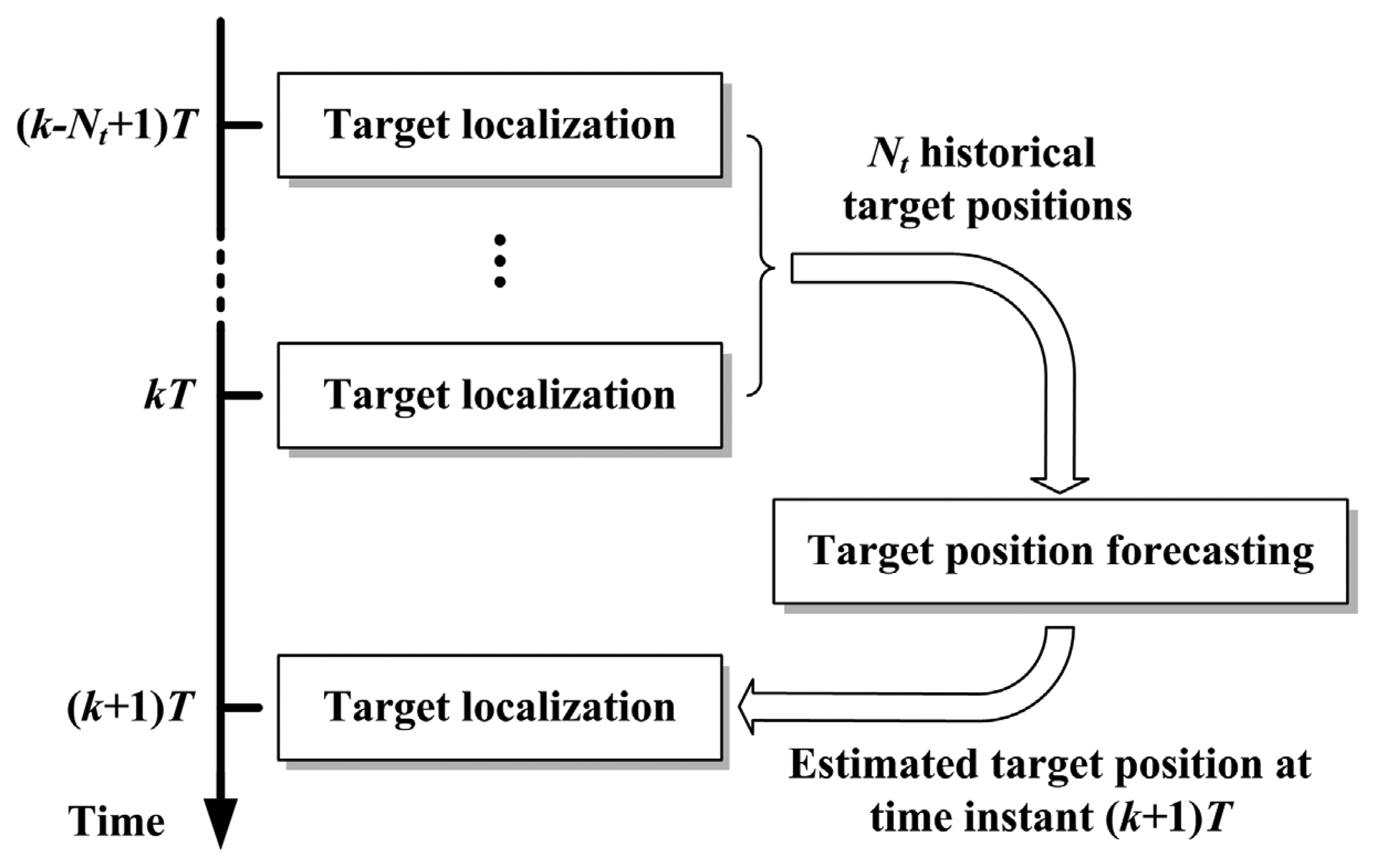
4.1. Target Forecasting by ARMA-RBF

As a record of the target trajectory, a time series of historical target position is transferred among the sensor nodes with sensing tasks. The data delivery approach will be discussed later in Section 4.2. When the current target position is obtained, the historical target is also available in the active sensor nodes so that target forecasting can be performed. In the two-dimension field, the target position is presented by Descartes coordinates. One direction of the target trajectory {y_k |k=1,2,⋯,N_t} is taken for discussion. The problem is to estimate the target position y_Nt+1 at the next sensing period. The same forecasting approach can be implemented on the other direction.

ARMA model is adopted here due to its outstanding performance in model fitting and forecasting and its lightweight computational cost. ARMA model contains two terms, the autoregressive (AR) term and the moving average (MA) term [38]. In the AR process, the current value of the time series y_k is expressed linearly in terms of its previous values {y_k−1,y_k−2,⋯, y_k−p} and a random noise a_k. This model is defined as a AR process of order p, AR(p). It can be presented as:

$$y_k={\varphi }_1{y}_{k-1}+{\varphi }_2{y}_{k-2}+\cdots +{\varphi }_p{y}_{k-p}+a_k$$

(14)

where {ϕ|i=1,2,⋯,p} are the AR coefficients. In the MA process, the current value of the time series y_k is expressed linearly in terms of current and previous values of a white noise series {a_k, a_k−1,⋯,a_k−q}. This noise series is constructed from the prediction errors. This model is defined as a MA process of order q, MA(q). It can be presented as:

$$y_k=a_t-{\theta }_1{a}_{k-1}-{\theta }_2{a}_{k-2}-\cdots -{\theta }_q{a}_{k-q}$$

(15)

The backshift operator B is introduced here. It is defined that

$$y_{k-i}=B^i{y}_k,a_{k-i}=B^i{a}_k$$

(16)

and

$$\mathrm{\Phi }(B)=1-{\varphi }_{1}B-{\varphi }_2{B}^2-\cdots -{\varphi }_p{B}^p$$

(17)

$$\mathrm{\Theta }(B)=1-{\theta }_{1}B-{\theta }_2{B}^2-\cdots -{\theta }_q{B}^q$$

(18)

Then, the AR process can be written as:

$$\mathrm{\Phi }(B)y_k=a_k$$

(19)

while the MA process can be written as:

$$y_k=\mathrm{\Theta }(B)a_k$$

(20)

In the autoregressive moving average process, the current value of the time series y_k is expressed linearly in terms of its values at previous periods {y_k−1, y_k−2,⋯,y_k−p} and in terms of current and previous values of a white noise {a_k, ay_k−1,⋯,a_k−q}. The order of the ARMA process is selected by both the oldest previous value of the series and the oldest white noise value at which y_k is regressed on. For this ARMA of order p and q, ARMA (p,q), it can be written as:

$$\mathrm{\Phi }(B)y_k=\mathrm{\Theta }(B)a_k$$

(21)

To determine the order of ARMA model, the patterns of autocorrelation function (ACF) and partial autocorrelation function (PACF) are analyzed. After experimental analysis, it is found that the time series {y_k | k=1,2,⋯,N_t} can be modeled by AR(p).

The method of least square estimation is adopted to determine the coefficients of AR(p) [39]. A linear equation can be acquired as follow:

$$Y_1=Y_{2}B+A$$

(22)

where Y₁ = [y_p+1 y_p+2 ⋯ y_Nt]^T, and

$$Y_2=\left[\begin{array}{cccc}{y}_p& y_{p-1}& \cdots & y_1\\ y_{p+1}& y_p& \cdots & y_2\\ ⋮& ⋮& \ddots & ⋮\\ y_{N_t-1}& y_{N_t-2}& \cdots & y_{N_t-p}\end{array}\right]$$

(23)

Besides, B=[ϕ₁ ϕ₂ ⋯ ϕ_p]^T is the coefficient vector, A = [a_p+1 a_p+2 ⋯ a_Nt]^T is the noise vector. Here, {ϕ_i |i = ϕ₂ 1,2,⋯, p} are the coefficients of AR(P) and {a_i | i = p+1, p+2, ⋯,N_t} are previous values of a white noise series.

Then the least square estimation of coefficients is:

$$\stackrel{⌢}{B}={(Y_2^T{Y}_2)}^{-1}{Y}_2^T{Y}_1$$

(24)

With the constructed AR(p) model, forecasting can be performed on sensor nodes. In general, the estimation equation of y_Nt+1 is:

$$E[y_{N_t+1}]={\varphi }_1{y}_{N_t}+{\varphi }_2{y}_{N_t-1}+\cdots +{\varphi }_p{y}_{N_t-p+1}$$

(25)

Compared to Equation (14), the noise term a_p+1 is not taken into account. To enhance the accuracy and robustness of forecasting, the estimation ȃ_p+1 of a_p+1 is obtained by RBFN here.

Radial basis functions (RBF) are a special class of function. Their characteristic feature is that their response decreases (or increases) monotonically with distance from a central point [40]. The centre, the distance scale and the precise shape of the radial function are parameters of the model, all fixed if it is linear. In principle, they could be employed in any sort (linear or nonlinear) of model and any sort (single-layer or multi-layer) of network. RBFN is a three-layer feed-forward neural network which is embedded with several radial-basis functions. Such a network is characterized by an input layer, a single layer of nonlinear processing neurons, and an output layer. The output of the RBFN is calculated according to [5]:

$$z_{\mathit{\text{out}}}=\sum _{j=1}^M{\omega }_j{\chi }_j(\Vert z_{in}-c_j{\Vert }_2)$$

(26)

where z_in is an input vector, χ_j is a basis function, ‖ · ‖₂ denotes the Euclidean norm, ω_j are the weights in the output layer, M is the number of neurons in the hidden layer, and c_j are the centers of RBF in the input vector space. The functional form of χ_j is assumed to have been given, which is always assumed as Gaussian function:

$$\chi \left(z_{in}\right)=e^{-\frac{z_{in}^2}{{\sigma }^2}}$$

(27)

where σ is a constant.

For ARMA-RBF, the RBFN is constructed according to Equation (26):

$${\stackrel{⌢}{a}}_{N_t+1}=\sum _{j=1}^M{\omega }_j{\chi }_j({\Vert y_{N_t-p+1:N_t}-c_j\Vert }_2)$$

(28)

Input vector [y_i y_i+1 ⋯ y_i+p−1] and output a_i+p are taken as the training samples, where 1≤ i ≤ N_t−p. Then the estimation y̑_Nt+1 is calculated as:

$${\stackrel{⌢}{y}}_{N_t+1}={\varphi }_1{y}_{N_t}+{\varphi }_2{y}_{N_t-1}+\cdots +{\varphi }_p{y}_{N_t-p+1}+{\stackrel{⌢}{a}}_{N_t+1}$$

(29)

In ARMA-RBF algorithm, the RBFN is dynamically trained with the new target position in each sensing period. With the output of RBFN, the forecasting error of ARMA model can be compensated.

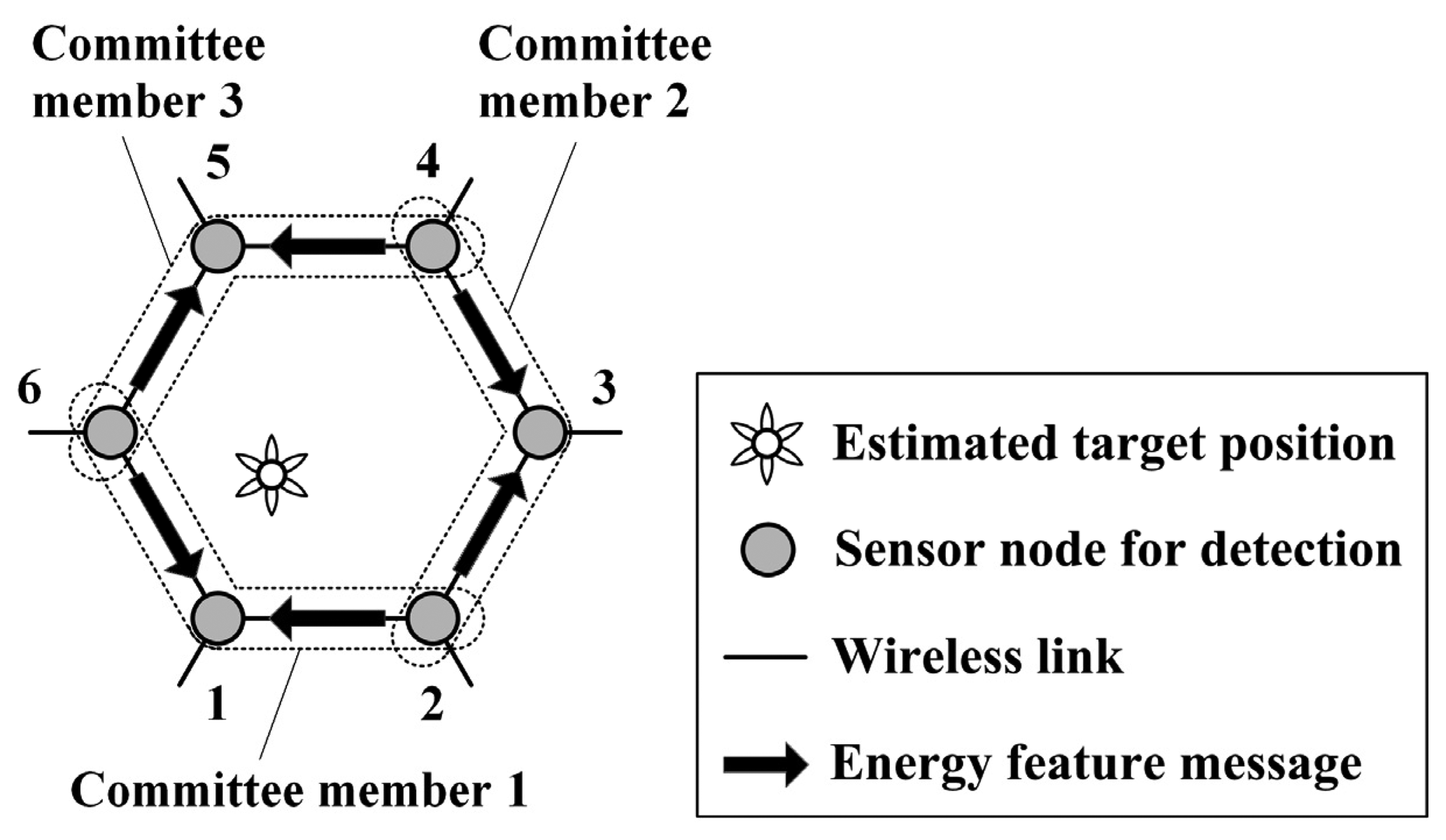
4.2. Target Localization with Committee Decision

With the target forecasting results, sensor nodes should be organized to perform future target localization. As described in Section 3.3, sensor nodes on the hexagon where the target is located will sense and localize the target. If the target is still in the same hexagon in the next sensing period, the sensor node will continue sensing in the next sensing period. Otherwise, the sensor node awakening should be performed as shown in Figure 5. Sensor nodes for current detection (sensor node A∼F) will awaken the sensor nodes for future detection (sensor node G∼J) according to the estimated target position.

In Figure 5, sensor node C and D will continue sensing in the next sensing period and accomplish the awakening task. After current detection, sensor node A, B, E and F will get into the sleep stage. Meanwhile, sensor node C and D still keep in the communication stage. Sensor node C sends the awakening message as well as the time information message to sensor node G. Then sensor node G is wakened to the communication stage and it update its clock with the time information from sensor node C. In the same way, sensor node G sends the awakening message and the time information message to sensor node H. Then sensor node I and J will be awakened one by one. Finally, sensor node J will send an ACK message to sensor node D. After that, a new cluster for future detection is established by sensor node C, D, G, H, I and J. Time synchronization is achieved in the cluster so that the acoustic signals associated with the same time interval can be discussed in the target localization procedure. These sensor nodes get into the sleep stage after sending messages and will awakened to the detection stage by their own timer in the next sensing period. Here, the communication energy consumption for awakening and time synchronization is ignored as the size of these messages is small.

In addition, the historical target positions should be delivered to the new cluster. In Figure 5, sensor node C or D should get the data. If the data is already on sensor node C or D, no data delivery is required. Otherwise, the sensor node which maintains the historical target information will send the data to sensor node C or D along the path with the least hops. For instance, sensor node F will choose the path FED if it has data to send.

In this way, six sensor nodes around the target will sense the acoustic signal simultaneously for each sensing period. As described in Section 3.1, target positions can be calculated from the energy of acoustic signal from multiple sensor nodes. According to Equation (7), the target position can be determined by the detection results of three sensor nodes. To reduce the overhead for centralized decision and overcome the detection uncertainty, an approach of committee decision is adopted. Committee decision is based on a commonly used engineering principle: divide and conquer [12]. A complex computational task is solved by dividing it into a number of computationally simple tasks and then combining the solutions to those tasks.

As shown in Figure 6, a committee of three members is established for target localization. Sensor nodes can obtain the energy features E_i(i=1,2,⋯,6) respectively, which represent the energy of received acoustic signal. It is assumed that sensor node 1 maintains the historical target information, so sensor node 1. Then sensor node 1 aggregates the energy features from sensor node 2 and 6. Meanwhile, sensor node 3 and 5 aggregate the energy features from the neighbors. Thereby, only sensor node 2, 4 and 6 need to broadcast their energy features and the divided localization task is assigned to three committee members.

First, each committee member should make local decision. Since the target localization task is time-critical, the analytical method is not feasible here. Still, the advantage of RBFN is considered. As the network structure is regular, a trained RBFN which expresses the mapping from energy features to target position can be integrated into each sensor node before deployment. Thus, any sensor node can make local decision when it has energy features from three different sensor nodes. As shown in Figure 7, the coordinate frame XOY. Each committee member should utilize a new coordinate frame for the generalization of RBFN. Taking the committee member 1 in Figure 6 for example, the new coordinate frame X′O′Y′ is constructed. The energy features from sensor node 1, 2 and 6 are E₁, E₂ and E₆, respectively, which are normalized as:

$$\begin{array}{cc}{E}_i^{\prime }=\frac{E_i}{\underset{k=1,2,6}{max}{E}_k}& i=1,2,6\end{array}$$

(30)

Any target position z′ = [x′ y′]^T is uniquely associated with a normalized energy feature vector $E^{\prime }={[E_1^{\prime }{E}_2^{\prime }{E}_6^{\prime }]}^T$ according to Equation (7). Following Equation (26), RBFN is constructed as:

$$z^{\prime }=\sum _{j=1}^M{\omega }_j{\chi }_j({\Vert E^{\prime }-c_j\Vert }_2)$$

(31)

Here, the training samples are generated according to Equation (7). Thus, committee member can acquire the target position z′ with this RBFN. Note that the coordinates [x′ y′]^T is the coordinates in the coordinate frame X′O′Y′. The target coordinates z = [x y]^T in the coordinate frame XOY is required in committee decision, which can be calculated as:

$$z=\left[\begin{array}{cc}cos\theta & sin\theta \\ -sin\theta & cos\theta \end{array}\right]z^{\prime }+\left[\begin{array}{c}{x}_1^s\\ y_1^s\end{array}\right]$$

(32)

where is ${[x_1^s{y}_1^s]}^T$ is the coordinates of sensor node 1 in the coordinate frame XOY. θ denotes the rotation angle between coordinate frame XOY and X′O′Y′. Assuming the coordinates of sensor node 2 is ${[x_1^s{y}_1^s]}^T$ in the coordinate frame XOY, we have:

$$sin\theta =\frac{y_1^s-y_2^s}{\sqrt{{(x_1^s-x_2^s)}^2+{(y_1^s-x_2^s)}^2}}$$

(33)

$$cos\theta =\frac{x_2^s-x_1^s}{\sqrt{{(x_1^s-x_2^s)}^2+{(y_1^s-x_2^s)}^2}}$$

(34)

Then, the committee decision is made with the local decision of committee members. See Figure 6, the committee members will obtain local results of target position ${[x_i^t,y_i^t]}^T(i=1,2,3)$ respectively. Sensor node 1 will receive the decisions from sensor node 3 and 5. Usually the decision of the committee is obtained by a weighted combination of the decisions of the committee members [41]. Here, the global result of target position [x^t, y^t]^T can be calculated as:

$$x^t=\frac{\sum _{i=1,2,3}{\omega }_i^t{x}_i^t}{\sum _{i=1,2,3}{\omega }_i^t},y^t=\frac{\sum _{i=1,2,3}{\omega }_i^t{y}_i^t}{\sum _{i=1,2,3}{\omega }_i^t}$$

(35)

where ${\omega }_i^t(i=1,2,3)$ denotes the weight of local decision. According to Section 3.1, the sensor node with higher value of energy feature is closer to the target. Since the uncertainty of detection is lower for the closer sensor node, the decision weight of committee member is defined as the sum of related energy features. In this case, we have:

$${\omega }_1^t=\sum _{i=1,2,6}{E}_i,{\omega }_2^t=\sum _{i=2,3,4}{E}_i,{\omega }_3^t=\sum _{i=4,5,6}{E}_i$$

(36)

where E_i(i=1,2,⋯,6) is the energy feature obtained by each sensor node. The data amount during committee decision is small, so the related energy consumption of communication is ignored. With knowledge of the past and current target positions, sensor node 1 can perform target forecasting for the next sensing period. This procedure is iterated when the target moves in sensing field.

Due to the symmetry of network structure, the above-mentioned approaches can be extended to general cases during target tracking. Sensor node awakening and data delivery ensure that only the sensor nodes around the target need to perform target detection and processing every sensing period. Thereby, most sensor nodes can keep in the sleep stage to save energy. Committee decision allows the sensor node make decision in a distributed way and overcomes the uncertainty of detection results.

4.3. Sensor-to-observer Routing Scheme

Except localizing the target, the target tracking application includes another important task: reporting the target motion information when any observer sends queries for it [42]. The observer can be located in any position of network. It injects the query into the network through the closest sensor node. Then this sensor node will spread the query simply by flooding. During the flooding procedure, the sensor nodes will awaken their neighbors for a short time and announce the message. Once the query is received by a sensor node that carries the latest target information, it will attempt to send the data of historical target positions back to the observer. Here, the routing scheme for the sensor-to-observer data transmission will be discussed.

As the honeycomb configuration is adopted, another convenient coordinate frame is introduced for the whole network [37]. As shown in Figure 8, axes of the coordinate frame parallel to three edge directions of honeycomb mesh while the position of one specified sensor node is taken as the coordinate origin. In the honeycomb mesh, edges going from a sensor node to its neighbors indicate unit vectors along the positive or negative direction of the axes. The sensor node carrying the latest target information is defined as source sensor node while the closest sensor node to the observer is defined as destination sensor node. In Figure 8, the positions of the source sensor node and observer sensor node are denoted by [−2 0 1]^T and [−1 −2 3]^T respectively.

The problem is to find a proper path from the source sensor node to the destination sensor node. For generalization, it is assumed that the position of source sensor node is [u₁ v₁ w₁]^T and the position of destination sensor node is [u₂ v₂ w₂]^T. Then, it can be found that the shortest path between the two sensor nodes contains |u₁−u₂| hops along the X₀ axis, |v₁− v₂| hops along the Y₀ axis, and |w₁−w₂| hops along the Z₀ axis. Here, the related directions are determined by the sign of (u₁ −u₂), (v₁ −v₂) and (w₁−w₂). Usually, there are multiple paths. For example, there are three paths from the source sensor node to the destination sensor node.

To prolong the lifetime of the whole sensor network, the residual energy of sensor node is considered. As the position of the destination sensor node is spread, so the source sensor node maintains Δ_S=[u₂− u₁ v₂−v₁ w₂−w₁]^T. There are three sensor nodes that can be next hop of source sensor node. Source sensor node will choose each sensor node with a probability:

$$\mathit{\text{prob}}(i)=\{\begin{array}{cc}0& \Vert \mathrm{\Delta }s+\mathit{\text{hop}}(i){\Vert }_2\ge \Vert \mathrm{\Delta }s{\Vert }_2\\ \frac{E_r(i)}{E_r^{\mathit{\text{sum}}}}& \Vert \mathrm{\Delta }s+\mathit{\text{hop}}(i){\Vert }_2<\Vert \mathrm{\Delta }s{\Vert }_2\end{array}$$

(37)

where ‖·‖₂ denotes the Euclidean norm, hop(i) is the vector going from the source sensor node to the specified neighbor i, and E_r(i) denotes the residual energy of the neighbor. In addition, $E_r^{\mathit{\text{sum}}}$ indicates the total residual energy of neighbors that satisfy ‖Δs+hop(i)‖₂<‖Δs‖₂. If the source sensor node transmits the data to the neighbor k, this neighbor will update Δs as:

$$\mathrm{\Delta }s=\mathrm{\Delta }s+\mathit{\text{hop}}(k)$$

(38)

Then it will choose its next hop in the same way. This procedure is iterated until the data is received by the destination sensor node. Finally, the observer can acquire the data from the destination sensor node. Thereby, the sensor nodes with lower energy are protected, the balance of energy distribution can be achieved in WMSN.

The proposed approaches of target forecasting and localization as well as data reporting are implemented in a distributed manner. Both the localization accuracy and energy efficiency are considered during the tracking procedure. Generally, each sensor node only needs to know the information of its neighbors. Even when it joins the cluster for the target localization, the information of other five sensor node is required to be maintained. In this way, the scalability and flexibility of WMSN are guaranteed.

5. Experimental Results

In this section, the efficiency of the proposed energy-efficient target tracking method will be evaluated by acoustic signal processing and energy consumption analysis in WMSN.

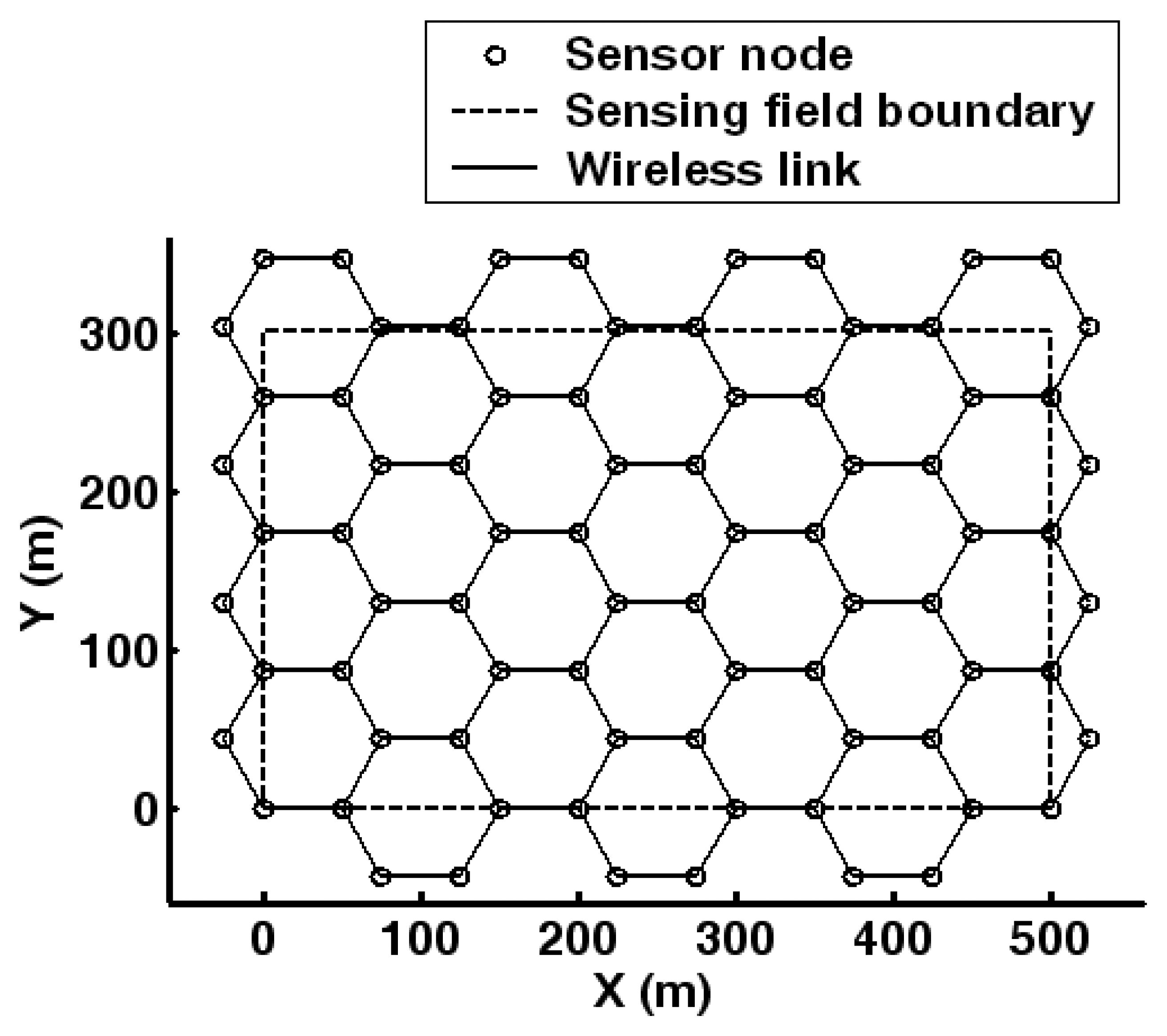
5.1. Experimentation Platform

It is assumed that a sensing field of 300 m×500m should be covered by WMSN. The sensing period for target detection is 0.5 s. First, the radio component of sensor node is defined referring to [12] and [43]. In Equation (9), the gain of transmitter G_t = 2, the gain of receiver G_r = 2, the radio wavelength λ = 0.125m, and the system loss factor β = 1. Moreover, the receiving power threshold P_th is defined as 6.04×10⁻⁹. The data rate of transmission is 400 kbit/s. The communication energy consumption is mainly derived from delivery and reporting of the historical target positions. It is assumed that the data packet size is 500 Byte. During the target localization, sensor nodes keep in the detection and communication stage for 80ms and 20 ms. When sensor nodes report the data of historical target positions to the observer, they only stay in the communication stage for data transmission.

The sensor nodes are deployed to establish the WMSN. Here, the communication range should be chosen to provide proper network density. As the network density mainly influences the data reporting procedure, so the related transmission latency and energy consumption is analyzed. WMSN is constructed with different communication range, while 500 pairs of observer and source sensor node positions are generated randomly. With the communication range varying from 20 m to 70 m, Figure 9 shows the transmission latency and energy consumption. The transmission latency is defined as the time from the source sensor sends out data to the time that the observer receives the data. It can be calculated as:

$$t_l=n_{\mathit{\text{hop}}}\cdot (\frac{M_D}{r_D}+t_w)$$

(39)

where n_hop is the hop number of data transmission, r_D is the data rate, M_D is the data packet size, and t_w is the transition time from the sleep stage to the communication stage. Meanwhile, the energy consumption is calculated according to Equation (11).

Here D_r denotes the Euclidean distance between the observer and source sensor node. The average values of transmission latency and energy consumption are illustrated for different interval of D_r. As shown in Figure 9(a), shorter communication range will lead to more hops for data reporting so that the time latency is larger. When D_r becomes larger, the transmission latency rises linearly. In Figure 9(b), the energy consumption is derived from processor and radio components. During data reporting, more hops imply that more sensor nodes should be awakened. Meanwhile, longer communication range will result in larger transmission energy. If D_r is large, the total energy consumption is impacted by the awakened sensor node number. Otherwise, it is impacted by the transmission energy consumption. When the communication range becomes larger than 50 m, energy consumption has no evident reduction or even it increases. As described in Section 3.3, the effective sensing range of sensor node is about 100 m in the vehicle detection. Thus, the communication range of sensor node is set as 50 m here.

According to the communication range of sensor node, the deployment of WMSN is given in Figure 10. There are 78 sensor nodes with honeycomb configuration while the sensing field is fully covered.

Thereby, any target moving in the sensing field can be detected by six sensor node on a hexagon at any time instant. For the coordinate frame described in Section 4.3, the coordinate origin is associated with the position (0 m, 0 m) in Figure 10.

In the experiments, the data of acoustic signal is acquired by MICAz motes from MICAz mote developer's kit (a commercial product of Crossbow Inc.) [44]. The MICAz is a 2.4GHz, IEEE 802.15.4 compliant module used for WSNs. The mote offers sensor boards that can measure signals such as acoustic, acceleration and so forth. Moreover, the MICAz motes are programmed to sample at the frequency of 4.96 kHz for acoustic signal acquisition. A truck is taken as the target and the trajectory is shown in Figure 11. The points on the trajectory are recorded according to the sensing period. The truck keeps moving in the sensing field for 120 s while the acoustic signals are acquired by the motes.

With the WMSN structure and acoustic signals, several experiments will be carried out to analyze the energy-efficient target tracking method. The acoustic signals are acquired from the real world experiments and the energy consumption will be evaluated by network simulations.

5.2. Target Localization Experiment

Assuming that the sensor node around the target can be awakened on time every sensing period, the target localization approach is discussed first.

As described in Section 4.2, a common RBFN should be established. The RBFN is constructed as Equation (31). According to Figure 7, target positions are generated randomly in the region for target localization. Then the theoretical values of normalized energy features are calculated with Equation (7) and (30). These energy features and target positions are regarded as training samples. Here, 200 training samples are taken and the mean squared error goal is set as 0.001.

With this trained RBFN, the local decision of target position can be obtained by a single committee member. Along the target path, the acoustic signal from the sensor node on related hexagon will be analyzed. For each sensing period, the sensor node acquires a sequence of signal amplitude in the detection stage. According to the detection time and sampling frequency given in Section 5.1, the number of sample points is 396. Thereby, the normalized energy feature can be obtained following Equation (30). For instance, the acoustic signals from related sensor nodes are shown in Figure 12 when the target is located at (307.7 m, 237.6 m). For signal 1 to 6, the associated sensor nodes are located at (300.0 m, 173.2 m), (350.0 m, 173.2 m), (375.0 m, 216.5 m), (350.0 m, 259.8 m), (300.0 m, 259.8 m) and (275.0 m, 216.5 m) respectively.

Here, the committee member 1 obtains the signal 1, 2 and 6; the committee member 2 obtains the signal 2, 3 and 6; and the committee member 3 obtains the signal 4, 5 and 6. The normalized energy features of each committee member are given by Figure 13. For each committee member, a new coordinate frame X′O′Y′ is established according to Figure 7. In X′O′Y′, the signals from the sensor nodes which are located at (0 m, 0 m), (50.0 m, 0 m) and (-25.0 m, 43.3 m) are denoted by signal I, II and III respectively. Taking the normalized energy features as input, the local decision of each committee member can be obtained by the RBFN. In this case, the results of target position are (305.4 m, 241.4 m), (304.6 m, 241.5 m) and (309.4 m, 236.7 m) for committee member 1, 2 and 3 respectively. The committee decision is (307.7 m, 238.5 m) according to Equation (35) and (36). It can be found that the committee decision get better results than the local decisions. Further investigation is performed to analyze the target localization with committee decision. With the target trajectory of Figure 11, the decisions of committee and single committee member are compared every sensing period. The target localization error is compared in Figure 14. Here, the decision of single committee member is made by the sensor node carrying the historical target information and its neighbors. Committee decision leads to higher accuracy of target localization.

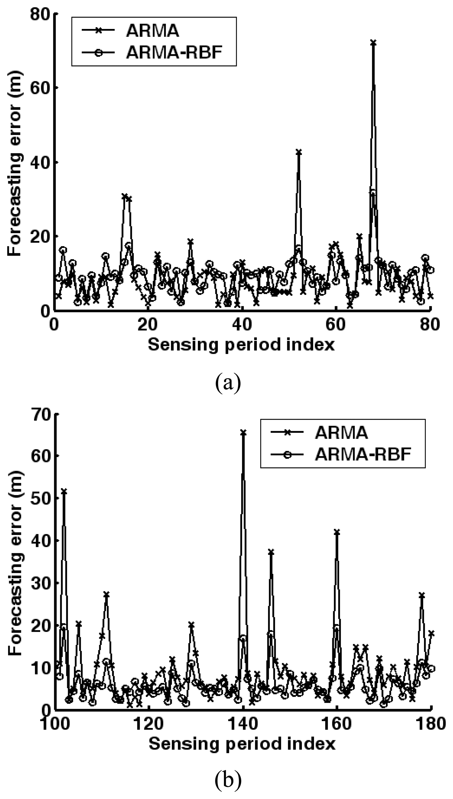
5.3. Target Position Forecasting Experiment

The efficiency of ARMA-RBF prediction is analyzed in this section. The target trajectory in Figure 11 is utilized here. The 61st to 180th sensing period is taken to show the performance of ARMA-RBF algorithm. For each sensing period, the sensor node carrying the historical target information will perform target forecasting after current detection.

According to Section 4.1, the error of target positions forecasted by ARMA and ARMA-RBF is compared in Figure 15, where the forecasting error in the X and Y directions of the coordinate frame XOY is shown. Following the patterns of ACF and PACF, the parameter p is set as 4 for AR(p) model. ARMA-RBF produces much less error than ARMA does. That is because the noise term of ARMA is predicted by RBFN and dynamic compensation achieves the robust forecasting performance. Thereby, it will provide more accuracy forecasting results for the observer and the awakening procedure as well.

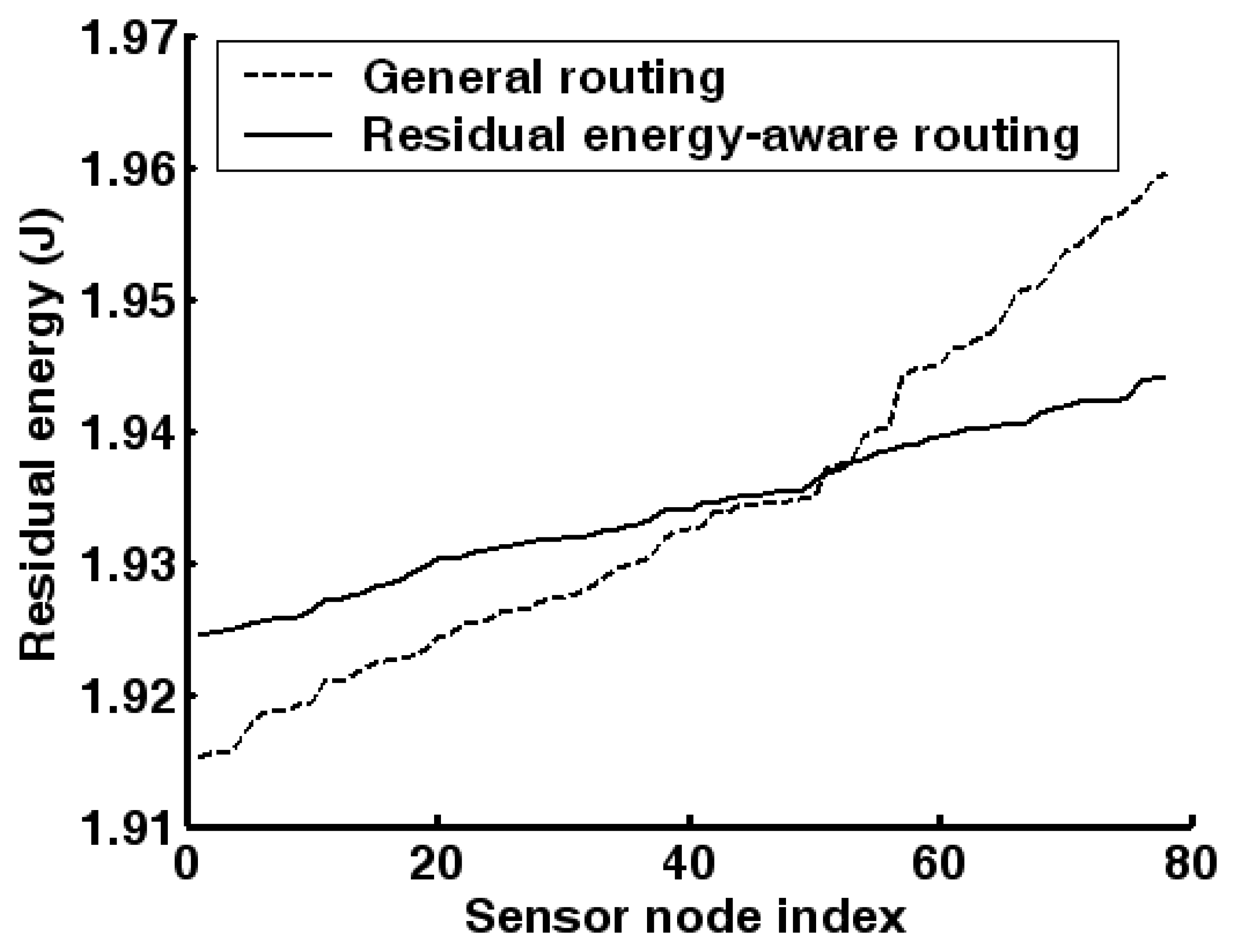
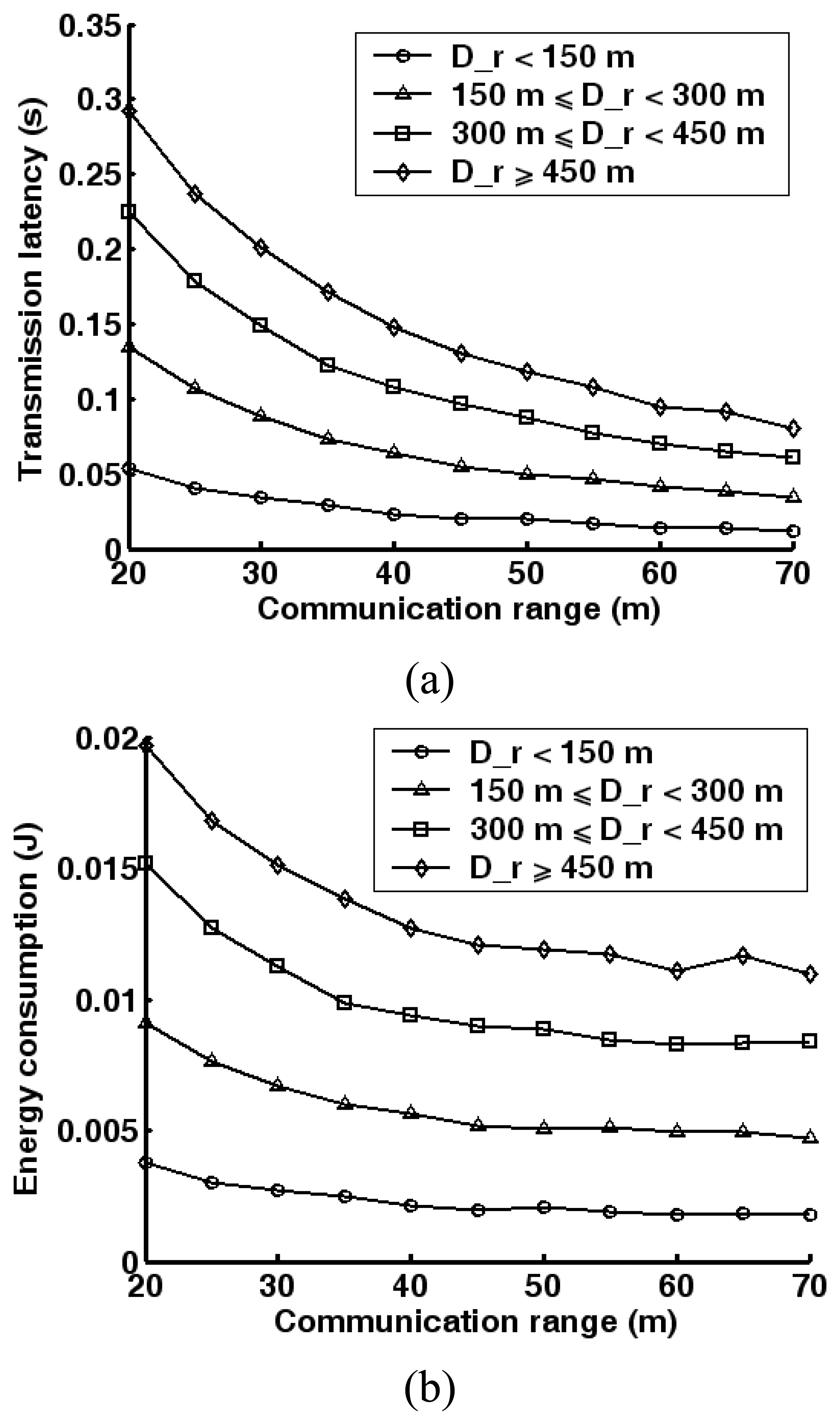
5.4. Energy Efficiency Analysis

In this section, energy efficiency of WMSN is evaluated. First, the energy consumption for sensor nodes staying in detection and communication for target detection is analyzed. The target moves in the sensing field as shown in Figure 11. Once it moves into one hexagon, the related six sensor node will be awakened to implement target localization and forecasting tasks. The awakening approach is simulated. Power consumption curve of the whole WMSN is given, which is calculated as:

$$P^{\mathit{\text{WMSN}}}(t)=\sum _{i=1}^{78}{P}_i^s(t)$$

(40)

where $P_i^s(t)$ is the power consumption of sensor node i at time instant t. It can be found that the average power consumption is quite stable in each sensing period. That is because the number of sensor node for detection is constant. Only when the target moves from one hexagon to another, there may be extra power consumption for data delivery. With 72 out of 78 sensor nodes (92.3%) staying in the sleep stage every sensing period, the average power is 40.8 mW, which is even lower than the power consumption of a single sensor node with its all components on. Thereby, WMSN obtains significant energy saving.

Moreover, the energy consumption during data reporting is evaluated according to Equation (12). Here, the sensor-to-observer routing scheme is adopted. Similar to Section 5.1, 500 pairs of observer and source sensor node positions are generated randomly. Thus, 1000 data reporting tasks should be accomplished. In addition, another routing scheme is taken for comparison, where sensor nodes have equal probability to choose a potential sensor node approaching the destination sensor node for the next hop. It is assumed that the initial energy of each sensor node is 2 J. See Figure 16, the residual energy distribution of sensor nodes in WMSN is presented after accomplishing data reporting tasks. The residual energy is sorted from low to high. It can be found that better balance of residual energy is achieved by the residual energy-aware routing. The balance of residual energy in each sensor node will help to delay the excessive energy depleting in a particular sensor node, and hence delay the unsuitability of the network topology.

In the experiments, target localization and forecasting is performed in a distributed way. Energy efficiency derived from sensor node awakening and sensor-to-observer routing scheme is evaluated. The efficiency of the proposed target tracking method is demonstrated in the specified scenario.

6. Conclusions

Focusing on the energy problems in the target tracking of WMSN, this paper has proposed a energy-efficient target tracking method. With robust target forecasting, the sensor nodes are awakened for target localization. The acoustic signal sensing model and energy consumption model are presented. A distributed network structure is defined with honeycomb configuration, where the coverage efficiency is justified with the limited communication range. With the historical target positions, the target position is forecasted by ARMA-RBF, where RBFN is utilized to compensate the ARMA forecasting. Sensor nodes of related hexagon are awakened every sensing period with the predicted target position. In particular, sensor nodes acquire the acoustic signals emitted by the target and target localization is achieved by committee decision. Committee is constructed with little communication overhead. Furthermore, a sensor-to-observer routing scheme is investigated for data reporting considering the residual energy of sensor nodes. Experimental results verify that the proposed target tracking method provide both robust localization performance and energy efficiency for WMSN. The main contribution of this paper is that a totally distributed framework and robust algorithms are designed for WMSN. The future research will focus on WMSN with heterogeneous sensors, such as image and seismic sensors. Hence, the corresponding signal process and fusion should be exploited.

References and Notes

1. Akyildiz, I.F.; Melodia, T.; Chowdury, K.R. A survey on wireless multimedia sensor networks. Computer Networks 2007, 51, 921–960. [Google Scholar]
2. Huang, H.C.; Huang, Y.M. An implementation of battery-aware wireless sensor network using ZigBee for multimedia service. Proceedings of International Conference on Consumer Electronics, Las Vegas, USA, Jan 7-11, 2006; pp. 369–370.
3. Liu, K.; Sayeed, A. M. Type-based decentralized detection in wireless sensor networks. IEEE Transactions on Signal Processing 2007, 55, 1899–1910. [Google Scholar]
4. Shin, J.; Chin, M. Optimal transmission range for topology management in wireless sensor networks. In Information Networking, Advances in Data Communications and Wireless Networks, Proceedings of the International Conference on Information Networking (ICOIN) 2006, Sendai, Japan, Jan 16-19, 2006; Chong, I., Kawahara, K., Eds.; pp. 177–185.
5. Wang, X.; Wang, S.; Ma, J. An improved particle filter for target tracking in sensor system. Sensors 2007, 7, 144–156. [Google Scholar]
6. Rao, S.K. Modified gain extended Kalman filter with application to bearings-only passive manoeuvring target tracking. IEE Proceeding-Radar, Sonar and Navigation 2005, 152, 239–244. [Google Scholar]
7. Song, C.; Sharif, H. Performance comparison of Kalman filter based approaches for energy efficiency in wireless sensor networks. Proceedings of the ACS/IEEE 2005 International Conference on Computer Systems and Applications, Jan 03 - 06, 2005; IEEE Computer Society: Washington, DC, USA; pp. 58–65.
8. Payne, O.; Marrs, A. An unscented particle filter for GMTI tracking. Proceedings of the IEEE Aerospace Conference 2004, Montana, Mar 6-13, 2004; pp. 1869–1875.
9. Zhang, H. Optimal and self-tuning State estimation for singular stochastic systems: a polynomial equation approach. IEEE Transactions on Circuits and Systems 2004, 51, 327–333. [Google Scholar]
10. Wies, R.W. Use of ARMA block processing for estimating stationary low-frequency electro-mechanical modes of power systems. IEEE Transactions on Power Systems 2003, 18, 167–173. [Google Scholar]
11. Lee, M.J.; Choi, Y.K. An adaptive neurocontroller using RBFN for robot manipulators. IEEE Transactions on Industrial Electronics 2004, 51, 711–717. [Google Scholar]
12. Wu, Q.; Rao, N.S.V. On computing mobile agent routes for data fusion in distributed sensor networks. IEEE Transactions on Knowledge and Data Engineering 2004, 6, 740–753. [Google Scholar]
13. Liang, S.; Hatzinakos, D. A cross-layer architecture of wireless sensor networks for target tracking. IEEE/ACM Transactions on Networking 2007, 15, 145–158. [Google Scholar]
14. Wang, X.; Ma, J.; Wang, S.; Bi, D. Prediction-based dynamic energy management in wireless sensor networks. Sensors 2007, 7, 251–266. [Google Scholar]
15. Fan, G.; Zhang, J. Maximizing sensor reuse based on new geometric concepts. Journal of Information Science and Engineering 2004, 20, 477–489. [Google Scholar]
16. Szewczyk, R.; Mainwaring, A. An analysis of a large scale habit monitoring application. Proceedings of the ACM Conference on Embedded Networked Sensor Systems 2004, Baltimore, Maryland, USA, Nov 3-5, 2004; pp. 214–226.
17. Simon, G.; Maroti, M. Sensor network-based countersniper system. Proceedings of the ACM Conference on Embedded Networked Sensor Systems 2004, Baltimore, Maryland, USA, Nov 3-5, 2004; pp. 1–12.
18. Arora, A.; Dutta, P. A line in the sand: A wireless sensor network for target detection, classification, and tracking. Computer Networks 2004, 46, 605–634. [Google Scholar]
19. Li, D.; Hu, Y.H. Energy based collaborative source localization using acoustic micro-sensor array. EURASIP Journal on Applied Signal Processing 2003, 4, 321–337. [Google Scholar]
20. Wang, X.; Bi, D.; Liang, D.; Wang, S. Agent collaborative target localization and classification in wireless sensor networks. Sensors 2007, 7, 1359–1386. [Google Scholar]
21. Li, D.; Wong, K.D.; Hu, Y.H.; Sayeed, A.M. Detection, classification and tracking of targets in distributed sensor networks. IEEE Signal Processing Magazine 2002, 19, 17–29. [Google Scholar]
22. He, T.; Krishnamurthy, S.; Luo, L. Vigilnet: An integrated sensor network system for energy-efficient surveillance. ACM Transactions on Sensor Networks 2006, 1–38. [Google Scholar]
23. Zhang, W.; Cao, G. Optimizing tree reconfiguration for mobile target tracking in sensor networks, Proceedings of the IEEE INFOCOM 2004, Hong-Kong, Mar 7-11, 2004; pp. 2434–2445.
24. Aslam, J.; Butler, Z.; Crespi, V. Tracking a moving object with a binary sensor network. Proceedings of the ACM Conference on Embedded Networked Sensor Systems 2003, Los Angeles, California, USA, Nov 5-7, 2003; pp. 150–161.
25. Duh, F.B.; Lin, C.T. Tracking a maneuvering target using neural fuzzy network. IEEE Transactions on System, Man, and Cybernetics 2004, 34, 16–33. [Google Scholar]
26. Zhao, F.; Shin, J. Information-driven dynamic sensor collaboration for tracking applications. IEEE Signal Processing Magazine 2002, 19, 61–72. [Google Scholar]
27. Liu, W.; Farooq, M. An ARMA model based scheme for maneuvering target tracking. Proceedings of the Midwest Symposium on Circuits and Systems 1994, Hiroshima, Japan, Jul 25-28, 2004; pp. 1408–1411.
28. Desouky, A.A.; Elkateb, M.M. Hybrid adaptive techniques for electric-load forecast using ANN and ARIMA. IEE Proceedings-Generation, Transmission and Distribution 2000, 147, 213–217. [Google Scholar]
29. Li, W.M.; Liu, J.W. The financial time series forecasting based on proposed ARMA-GRNN model. Proceedings of International Conference on Machine Learning and Cybernetics; 2005; pp. 2005–2009. [Google Scholar]
30. He, T.; Blum, B.M. AIDA: Adaptive application independent data aggregation in wireless sensor networks. ACM Transactions on Embedded Computing System, special issue on Dynamically Adaptable Embedded 2004, 426–457. [Google Scholar]
31. Du, X.; Lin, F. Efficient energy management protocol for target tracking sensor networks. Proceedings of the IEEE International Symposium on Integrated Network Management 2005, Nice, France, May 15-19, 2005; pp. 45–58.
32. Sheng, X.; Hu, Y. Energy based acoustic source localization. Proceedings of the ACM/IEEE International Conference on Information Processing in Sensor Networks 2003, Palo Alto, California, USA, Apr 22-23, 2003; pp. 285–300.
33. Dutta, P.; Grimmer, M. Design of a wireless sensor network platform for detecting rare, random, and ephemeral events. Proceedings of the ACM/IEEE International Conference on Information Processing in Sensor Networks 2005, Los Angeles, CA, USA, Apr 25-27, 2005; pp. 497–502.
34. Durte, M.; Hu, Y.H. Vehicle classification in distributed sensor networks. Journal of Parallel and Distributed Computing 2004, 64, 826–838. [Google Scholar]
35. Deb, B.; Bhatnagar, S.; Nath, B. A topology discovery algorithm for sensor networks with applications to network management. Technical Report, DCS-TR-441, Rutgers University 2001. [Google Scholar]
36. Krohn, A.; Beigl, M. Increasing connectivity in wireless sensor network using cooperative transmission. Proceedings of the International Conference on Networked Sensing Systems 2006, Chicago, IL, USA, May 31-Jun 2, 2006; pp. 1–8.
37. Stojmenovic, I. Honeycomb Networks: Topological Properties and Communication Algorithms. IEEE Transactions on Parallel and Distributed System 1997, 8, 1036–1042. [Google Scholar]
38. Broersen, P.M.T. Automatic identification of time-series models from long autoregressive models. IEEE Transactions on Instrumentation and Measurement 2005, 54, 1862–1868. [Google Scholar]
39. Biscainho, L.W.P. AR model estimation from quantized signals. IEEE Signal Processing Letters 2004, 11, 183–185. [Google Scholar]
40. Haykin, S. Neural Networks: a Comprehensive Foundation; Prentice Hall: NJ, USA, 1999. [Google Scholar]
41. Shi, M.H.; Amine, B. Committee machine with over 95% classification accuracy for combustible gas identification. Proceedings of the IEEE International Conference on Electronics, Circuits and Systems 2006, Nice, France, Dec 10-13, 2006; pp. 862–865.
42. Wang, X.; Wang, S. Collaborative signal processing for target tracking in distributed wireless sensor networks. Journal of Parallel and Distributed Computing 2007, 67, 501–515. [Google Scholar]
43. Chen, A.; Lee, D. HIMAC: High throughput MAC layer multicasting in wireless networks. Proceedings of the IEEE International Conference on Mobile Ad hoc and Sensor Systems 2006, oVancouver, Canada, Oct 9-12, 2006; pp. 41–50.
44. MICAz Datasheet; Crossbow Technology Inc.: San Jose, California, 2006.
Figure 1. Hardware configuration and transition order of sleep stage, detection stage and communication stage.
Sensors 07 02779f1
Figure 2. Communication coverage analysis of different network structures: (a) 3-neighbor; (b) 4-neighbor; (c) 6-neighbor.
Sensors 07 02779f2
Figure 3. WMSN framework and sensing approach for target tracking.
Sensors 07 02779f3
Figure 4. WMSN framework and sensing approach for target tracking.
Sensors 07 02779f4
Figure 5. Sensor node awakening approach with target forecasting.
Sensors 07 02779f5
Figure 6. Committee established for target localization.
Sensors 07 02779f6
Figure 7. Coordinate transformation for local decision of committee member.
Sensors 07 02779f7
Figure 8. Convenient coordinate frame for sensor-to-observer routing.
Sensors 07 02779f8
Figure 9. Data reporting performance analysis with different communication range: (a) Energy consumption; (b) Transmission latency.
Sensors 07 02779f9
Figure 10. Sensor node deployment and wireless links in WMSN.
Sensors 07 02779f10
Figure 11. Target trajectory for tracking in WMSN.
Sensors 07 02779f11
Figure 12. Acoustic signal from sensor nodes when the target is located at (307.7 m, 237.6 m).
Sensors 07 02779f12
Figure 13. The normalized energy of acoustic signal of the three committee members.
Sensors 07 02779f13
Figure 14. Comparison of target localization error with single committee member and the committee.
Sensors 07 02779f14
Figure 15. Target position forecasting error of ARMA and ARMA-RBF in the coordinate frame XOY: (a) X direction; (b) Y direction.
Sensors 07 02779f15
Figure 16. Residual energy distribution of sensor nodes in WMSN after accomplishing data reporting tasks.
Sensors 07 02779f16