Introduction
The development of platforms to deploy of analytical systems in the field has not kept pace with development of the analytical sensors. Researchers that develop new sensors eventually encounter the problem of supporting, communicating, calibrating and cleaning sensors deployed in the field. This lack of presenting a complete solution to the users slows, inhibits, and is often the “valley of death” for the use of sensor technologies. The development of a “universal platform” has greatly decreased the time and cost required to deploy analytical sensors for analyzing trace environmental contaminants in the field. The platform was designed in a “plug and play” configuration for several types of analytical systems including trichloroethene (TCE), carbon tetrachloride, volatile aromatics, hexavalent chromium and lead. The platform has previously been used to monitor for trichloroethene TCE, 1 to 200 ppb concentration range, using a TCE-specific optrode. The trichloroethene monitoring system has been used successfully in monitoring TCE treatment systems in Arizona and California [
1-
2], and in monitoring wells at an Air Force Base in California [
3].
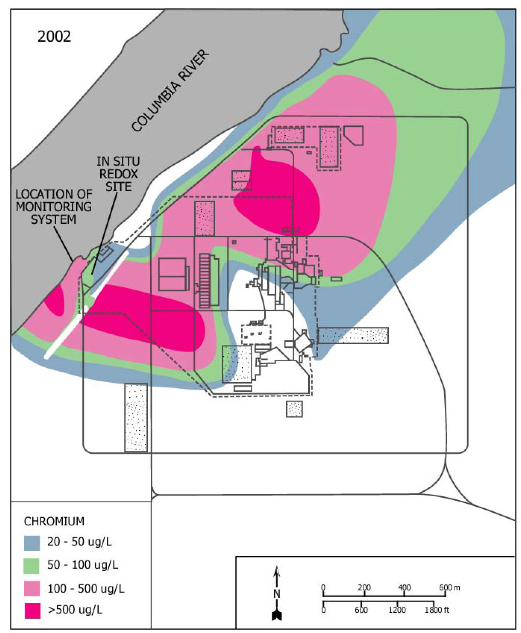
The platform was modified to monitor hexavalent chromium and conductivity from shallow groundwater wells (aquifer tubes) adjacent to the Columbia River at the 100-D Area of the Hanford Site, Washington [
4]. Sodium dichromate, the source of the hexavalent chromium, was formerly used at the 100-D Area to control corrosion in the piping of a nuclear reactor. Releases from the piping and other discharges resulted in soil and ground water contamination. A groundwater plume of hexavalent chromium is discharging through the riverbed and into the Columbia River (
Figure 1). Hexavalent chromium can be toxic to aquatic organisms; of special concern are the juvenile stages of salmon using the riverbed as spawning habitat.
To evaluate exposure risk for aquatic receptors, hexavalent chromium concentration data are needed (a) from a variety of river environment locations, and (b) at a frequency greater than that associated with traditional monitoring methods. The best location for monitoring concentrations is near the point of discharge to the river. Previous work has demonstrated successful methods for establishing access to shallow ground water using sampling ports and tubing that extends to onshore locations. The weakness of current monitoring capabilities is the impracticality of obtaining frequent hexavalent chromium measurements sufficient to characterize the temporal changes that occur in shallow ground water. These changes occur as a consequence of daily, weekly, and seasonal cycles in river discharge, which is controlled by upstream dams. A field-deployable, automated hexavalent chromium measurement system offered a means to fully characterize the conditions in this sensitive aquatic habitat. Key specifications for the system include: (a) practical quantitation limit of at least 5 ppb -- the relevant regulatory standard is 10 ppb; (b) ability to make at least hourly measurements; (c) field independence for at least two weeks; (d) provision for automated, internal calibration using standards; and (e) reasonable cost of operation when compared to the current costs of manual collection of field samples for laboratory analysis.
The Burge platform offered a simple solution to deploy a colorimetric system for the analysis of hexavalent chromium using 1,2-diphenylcarbazide. The diphenylcarbazide reagent is used in EPA methods for the analysis of hexavalent chromium. It was assumed that the more an analysis conforms to EPA protocols, the greater the probability of regulatory acceptance. Therefore, the colorimetric analysis was automated and interfaced to the sampling/calibration platform. This paper presents the design and preliminary performance data for an automated “universal” system. The automated system is capable of performing automated sampling, analysis and calibration without the requirement of a resident operator.
| “Universal”sampling/ analytical system |
| The system was developed and programmed to perform the following operations: |
| Sampling |
| Wells, surface water and treatment systems |
| Up to four ports: monitoring wells, surface water, etc. |
| Wells 2 inches and larger |
| Up to four depths in a single well (Multi-Level Sampling) |
| Low-flow sampling |
| Low energy requirements (solar cells) |
| Calibration and quality control |
| Creating blank water (for cleaning and calibration) |
| Three-point calibration curve |
| Standard additions |
| Mid-calibration checks |
| Spikes and splits |
| Analytical |
| Accommodating many types of sensors (TCE, Cr(VI), aromatics) |
| Operates of two sensor systems simultaneously with temperature and conductivity |
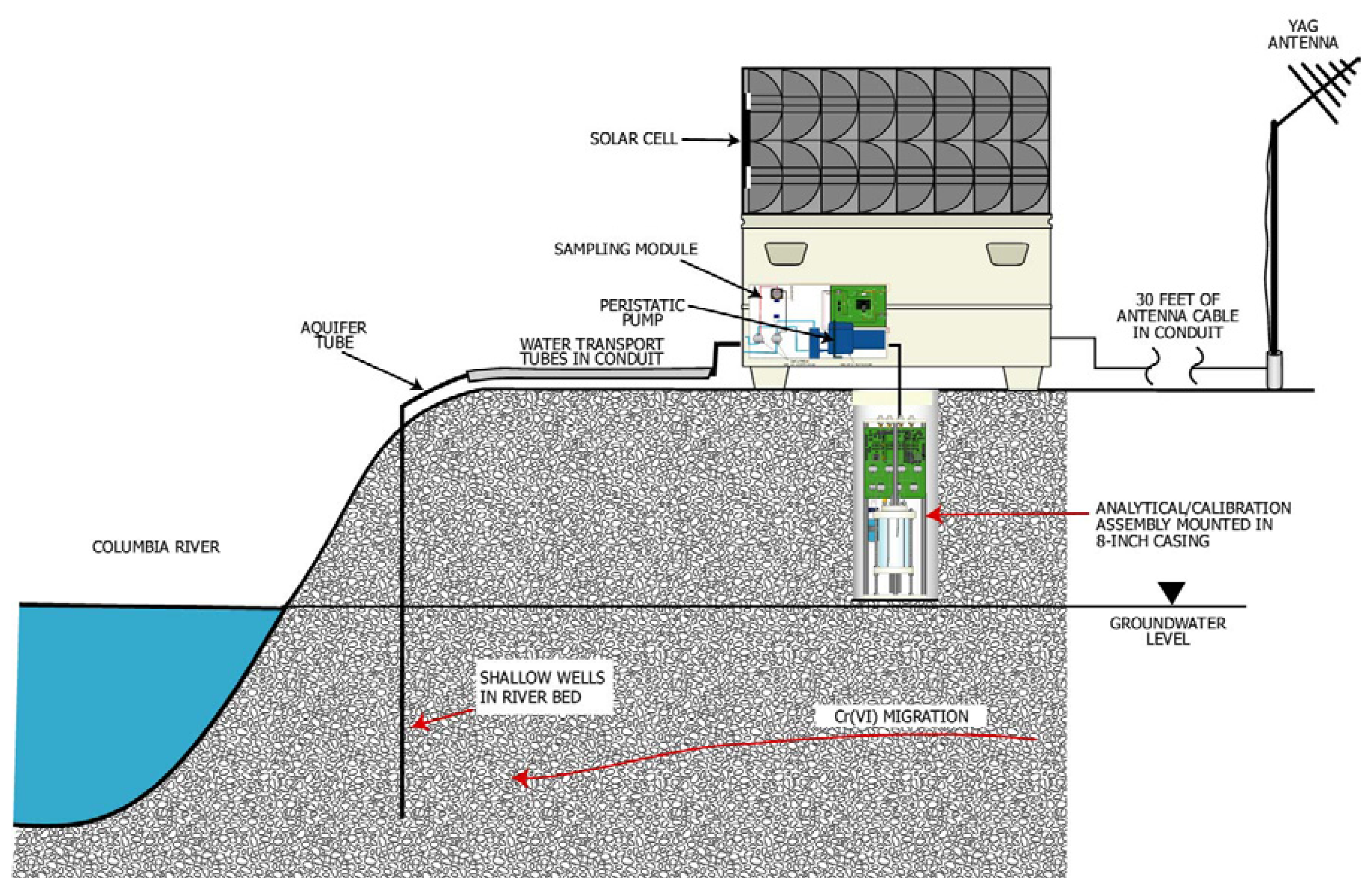
A diagram of the complete universal platform deployed in the field is illustrated on
Figure 2. The monitoring system is composed of several modules for sample collection, calibration, analysis, data acquisition/control, communication and waste treatment. The entire monitoring system was deployed in a field deployment box. The field deployment box is used to mount the solar cell panels and house the batteries, air system, and communication module. A 20.25-cm (8-in.) outside diameter (OD) casing passed through the bottom of the field deployment box and housed the analytical and calibration modules. The bottom of the casing extended approximately 90 cm (3 ft) into the soil. The analytical and calibration modules were mounted inside the well casing for temperature control.
Two 75-watt photovoltaic cells and a solar controller charged two 90 amp-hour sealed deep charge batteries. Compressed air operated many of the functions of the calibration and analytical modules. A 12-volt, 1/10-hp air compressor with an automatic pressure switch 8 to 10.9 kPa (55 to 75 psi) supplied air to a 19 cubic liter (5 cubic ft) tank. Two air regulators provided two levels of air pressure, 0.22 to 1.45 kPa (1.5 and 10 psi), to the calibration and analytical systems.
Sampling module
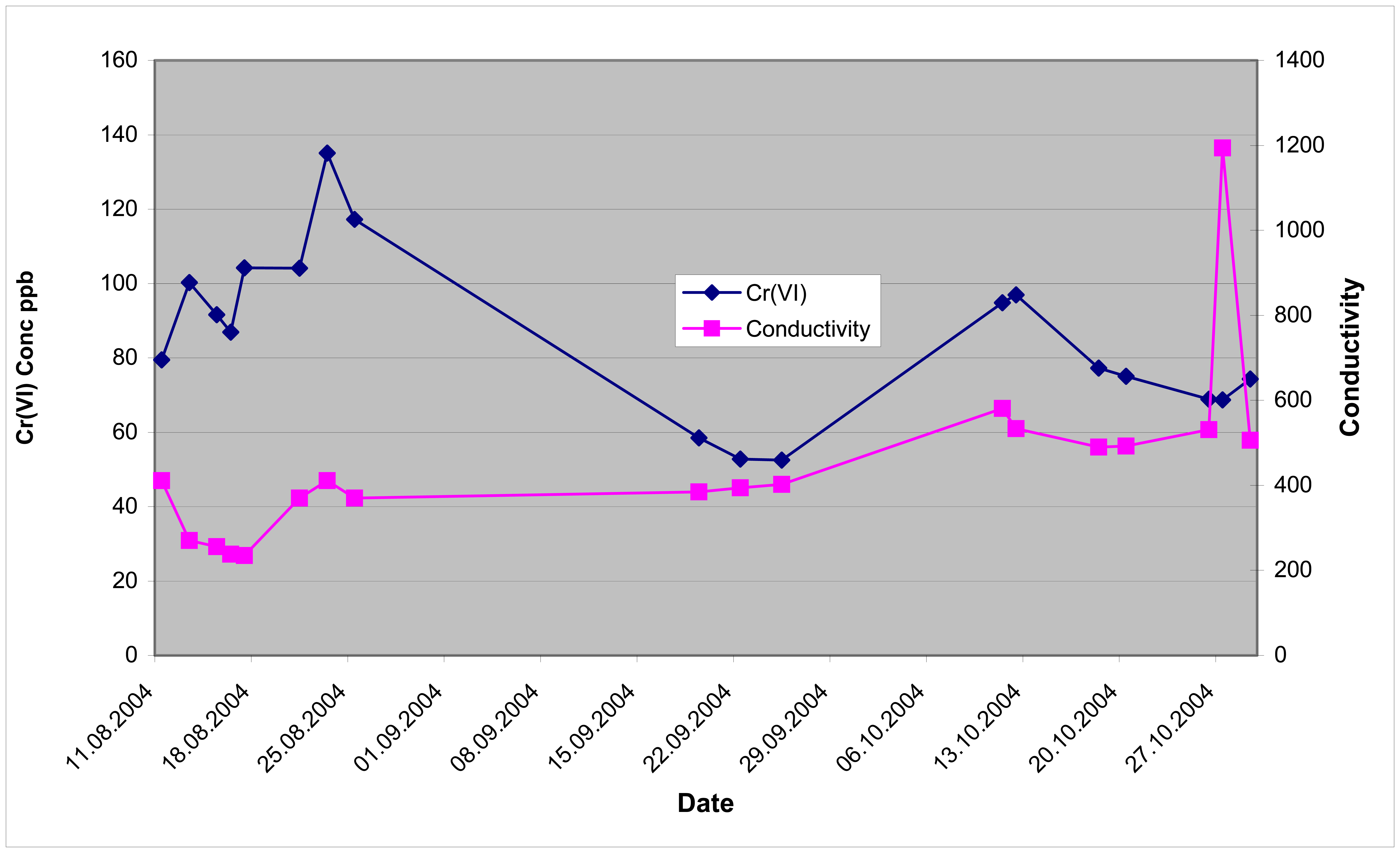
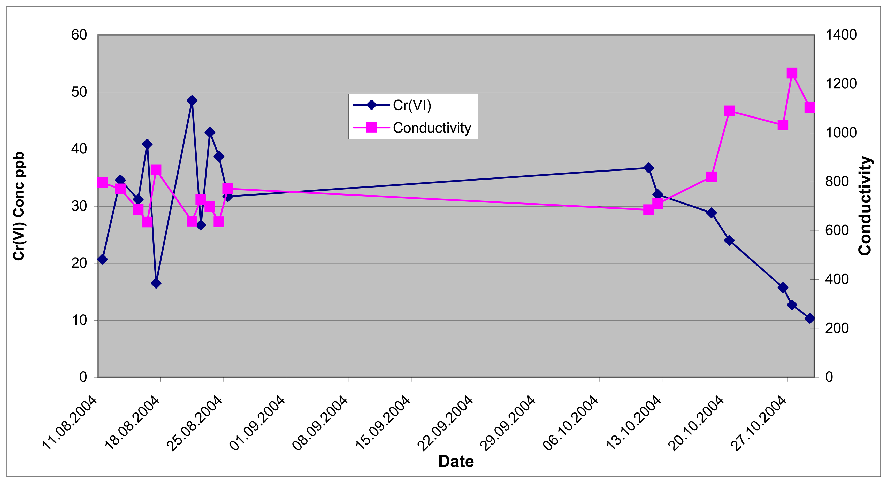
The water samples were collected from aquifer tubes placed into the banks of the Columbia River (
Figure 1). Two aquifer tubes (DD-39-1 and DD-39-3) were selected for the investigation. The entrance ports of the aquifer tubes (DD-39-1 and DD-39-3) were located 1.7 and 4.5 m below the surface of the riverbed. The aquifer tubes were 0.47 cm inner diameter (ID) polymer tubes with 15.2 cm stainless screens located at the terminal end of the tubes to prevent particles from entering the aquifer tubes. The tubes were installed in the cobble beach sediment of the river by advancing a temporary casing into the riverbed and inserting the aquifer tubes. The temporary casing was slowly withdrawn allowing the gravels to collapse around the aquifer tubes.
The distance between the field deployment box and the location of the aquifer tubes entered the subsurface was approximately 13 m. Fluorocarbon tubing (0.16 cm ID) was passed through the 0.47 cm ID aquifer tube from the stainless steel screen located in the subsurface to the field deployment box for transporting the sample to the sampling module. The sampling module was composed of four three-way sample selection valves and a peristaltic pump and was capable of monitoring up to five shallow wells. A monitoring program allowed the user to select the aquifer tube to be sampled by activating the corresponding sample selection valve, and the peristaltic pump that then drew in sample water into the analytical/calibration unit. Upon completion of a sampling episode, the three-way sample selection valve was deactivated, which opened a vent to the atmosphere and cleared the sample from the sample tube. This eliminated the contamination of the walls of the sample tube caused by prolonged storage of sample water in the tube.
Analytical / calibration assembly
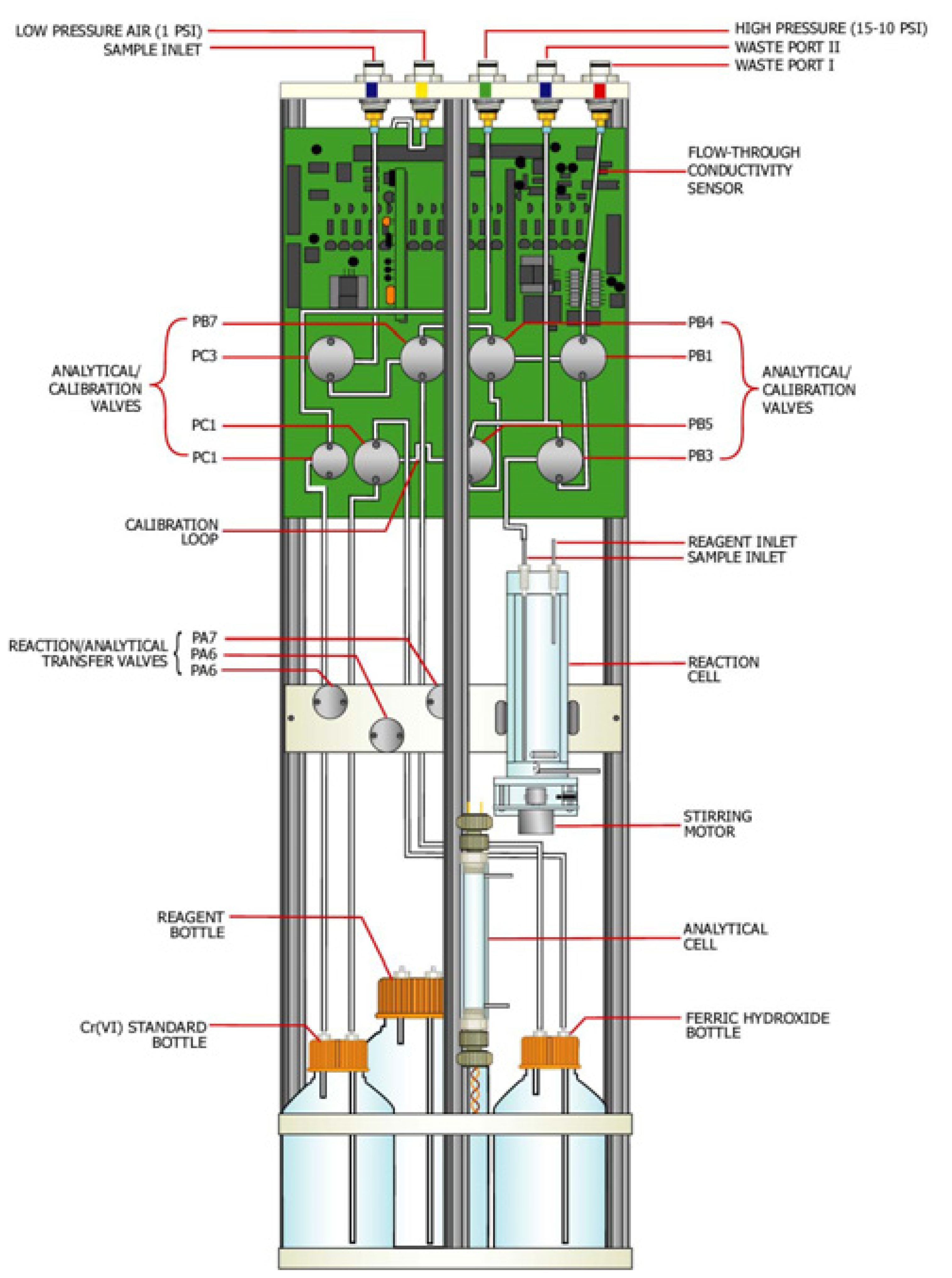
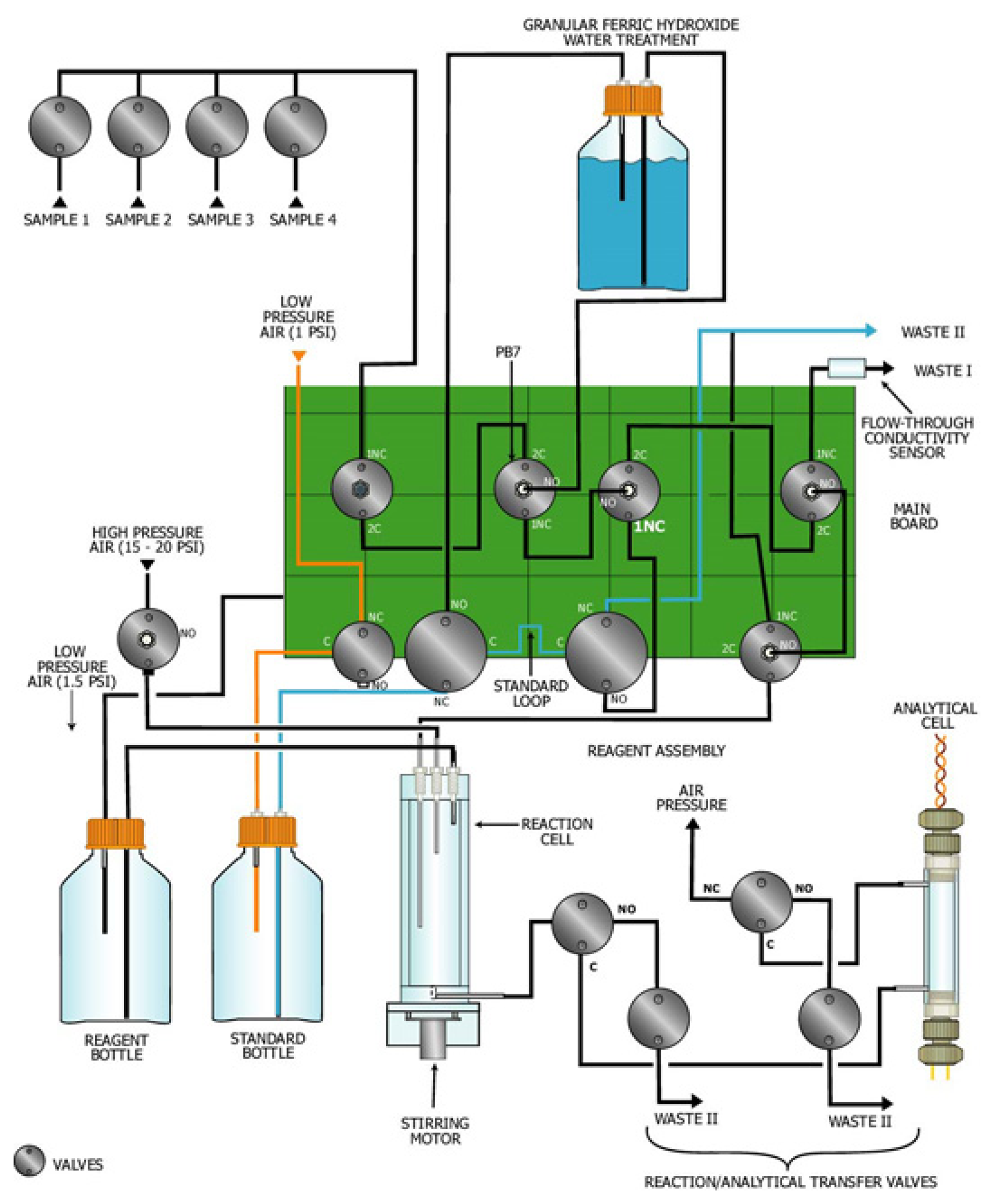
The analytical and calibration modules were combined in a cylindrical instrument 19.6 cm (7 3/4 in.) in diameter and 50.6 cm (20 inch.) high (
Figure 3). The instrument was cylindrical in shape to allow for installation into the 20.25 cm OD casing located under the field deployment box (
Figure 2). The analytical module was composed of the analytical cell, reaction cell, and the reagent delivery system. The calibration module was composed of several valves, and a hexavalent chromium removal (granular ferric hydroxide) and standard bottles. Schematic illustrations of the analytical and calibration modules are presented as
Figures 3 and
4.
Analytical module
The analytical module had two cells: reaction and analytical cells (
Figures 3 and
4). The sample reaction cell was used to mix the sample water with the colorimetric reagent forming a red solution. The resulting colored solution was transferred to the analytical cell for colorimetric measurement of the attenuation of a pulsed green light through the red solution. The analytical methodology is automated method of standard methods used in analysis of wastewater [
5].
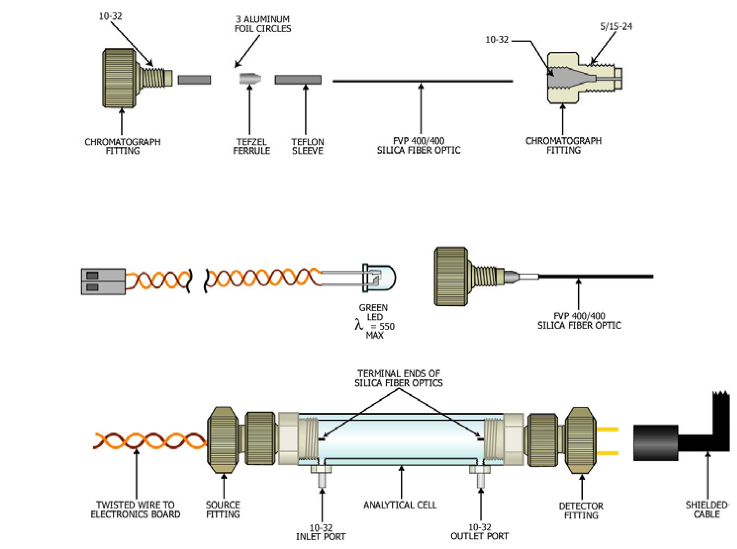
Analytical cell
Analytical cells were fabricated from a polycarbonate tube (1.26 cm, 0.5 in. ID) in lengths that varied from 1 to 15 cm (
Figure 5). The length of the cell was selected based on the hexavalent chromium concentration in the water to be monitored. A limit of detection of 0.5 ppb was attained for a 15-cm tube. A 4-cm tube with an effective path length of 3 cm was used in this investigation (30 to 120 ppb concentration range).
The analytical cell had 5/16-24 threads at the terminal ends of the tube and two ports with 10-32 threads located near the end of the tube. The 10-32 ports were used to introduce and drain the sample from the analytical tube. In addition, the 10-32 fittings served as electrodes for a conductivity detector for determining when the analytical cell was filled with sample.
The source and detector of the analytical cells were fabricated from commercially available polymer chromatography fittings that connected to the 5/16-24 threads at the ends of the analytical tube. The PEEK chromatography fittings (Upchurch Scientific, Oak Harbor, WA) were modified to allow a green light emitting diode (source) and a photodetector (detector) to be mounted in the body of the fittings. The light emitting diode had a λmax at 550 nm. A length of 400/400 silica fiber optic (Polymicro Technologies, Phoenix, AZ) was passed through the commercially available sleeves and ferrules to create watertight seals between the source and detector mounted in the fittings, and the sample contained in the analytical cell. Electrical cables connected the LED and photodetector to an electronic board for pulsing (30 Hz) the source and a lock-in amplifier to amplify and process the signal.
Reaction cell
The reaction cell was used to mix the reagent and sample (or standard). The reagent was 250 mg of the phenylcarbazide in 500 mL of 0.1 N HCl. The reaction cell was fabricated from 3/4-inch ID polycarbonate tube and three conductivity sensors to regulate the addition of the sample water and reagent. This investigation used 10 mL of sample water and 2.5 mL of reagent for each analysis. The reagent was stored in a 500-mL bottle for dispensing into the reagent chamber. The bottle had sufficient reagent to perform over 200 analyses.
The water sample was delivered to the reaction cell by the peristaltic pump and the reagent was delivered by pressurizing (1.5 PSI) the reagent bottle. The sample/reagent solution contained in the reaction cell was mixed with a small magnetic stirrer. After the reaction was complete, the reaction cell was pressurized (1.5 PSI), transferring solution to the analytical cell for colorimetric analysis. The reactivity of the reagent was variable and the hexavalent chromium signal attenuated over time because of the reagent stability. Reagent stability was compensated by the ability of the system to recalibrate at any time the reagent lost reactivity.
Calibration module
The calibration module performed two functions: creation of the blank water and creation of a three-step calibration curve. The calibration module had a three-way valve (Valve PB7 on
Fig. 3 and
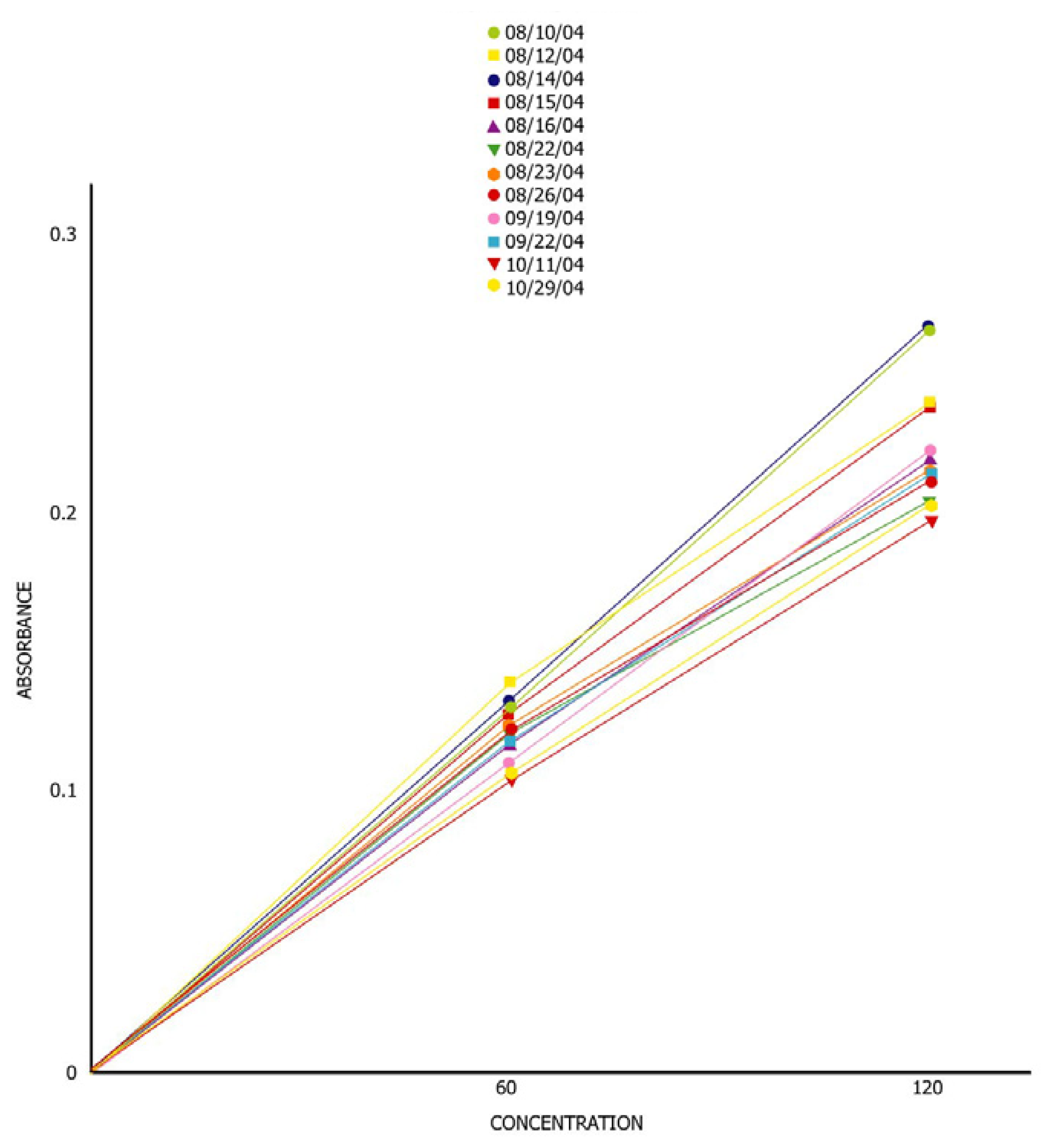
Fig. 4) to divert sample water directly to the analytical chamber or through the calibration module. Sample water diverted directly to the reaction chamber was used for analysis of the sample water. Sample water diverted to the calibration module was passed through a filter of granular ferric hydroxide to remove the hexavalent chromium from the water (the “blank water”). Blank water was used to clean the system and create the three-step calibration curve. The three-step calibration curve was created by injecting a stock chromium standard (2 mg/mL), using a calibration loop (0.3 mL), into the reaction cell. The program diluted the injected standard in the reaction cell with blank water to a total volume of 10 mL. The three-step calibration curve was constructed by analyzing blank, mid-value and high concentration standards. The mid-value standard was created by one injection of a loop volume into the reaction cell, and the high standard was created by two injections of a loop volume into the reaction cell. For this investigation, a hexavalent standard of 2 μg/mL was used to create a three-step calibration curve of 0, 60 and 120 ppb. The hexavalent chromium bottle contained 500 mL of stock standard capable of performing over 100 calibration curves. The hexavalent standard has been used for over 8 months in the laboratory without any significant decreases in the chromium signal.
Conductivity detector
After the first deployment, it was recognized that conductivity was an important parameter to be monitored in conjunction with hexavalent chromium. The design of the monitoring system was reviewed and it was recognized that a conductivity sensor used in the operation of the monitoring system could be adapted as a flow-through conductivity cell to provide conductivity data concerning the water being sampled. The design of the conductivity detector is not similar to commercially available detectors and was not optimized for highly accurate conductivity measurements. The conductivity detector incorporated into the system allowed users to determine whether the water being sampled through the aquifer tubes was from ground water or from the Columbia River. The water conductivity of the Columbia River is significantly lower than the conductivity of ground water. The operating program of the monitoring system was modified to allow the use of the conductivity cell. The location of the flow-through conductivity cell with the analytical/calibration assembly is illustrated on
Figures 3 and
4. The conductivity data were collected beginning with the second deployment on August 10, 2004.
Waste system
The waste system consisted of two water treatment canisters and a 210 liter (55-gallon) plastic drum to store the treated water. Two types of wastewater were produced during the operation of the monitoring system. Wastewater I was produced during purging of sample tubes from the entrance of the aquifer tubes located in the gravel bed of the river through the analytical/calibration system. Wastewater I contained low concentrations (30 to 200 ppb) of hexavalent chromium from the ground water. Wastewater I was passed through a canister of granular ferric hydroxide to remove the hexavalent chromium from the wastewater before discharge into the 55-gallon drum. Wastewater II was produced during analysis of water samples. Wastewater II contained hydrochloric acid with reacted and unreacted reagent. Wastewater II was passed through a canister containing marble chips and activated carbon to react with the acid and remove the reagent from the wastewater prior to discharge into the 55-gallon drum. Each sampling and analysis of a sample produced approximately 50 mL of water. Assuming the monitoring system can perform 200 analyses before the colorimetric reagent must be replenished, approximately 10 liters of wastewater is produced. However the actual amount of wastewater contained in the drum, over a field deployment of several months, was significantly less than the calculated wastewater produced because of evaporation.
Communication system
Communication between the remote user and the monitoring system was established with a spread spectrum frequency hopping radio modem (SRM6000, Data-Linc, Bellevue, Washington). A serial cable connected the modem located in the field deployment box to a small PLC (ADR-1000, Ontrack Control Systems, Sudbury, Ontario) located on the analytical/calibration unit. The monitoring system was controlled by a PC located at a remote location, a trailer was approximately ½ mile from the monitoring location. The program on the PC sent commands and received data via the modem from the PLC located on the analytical/calibration unit. The modem was capable of operating at distances of 12 miles. The PC located in the trailer was remotely controlled by users in Tempe, Arizona, using PC Anywhere™
Analysis and quality control
The monitoring system was designed to perform many of the analytical techniques used in fixed laboratories. The calibration system created and delivered blank (water), mid-value, and high concentration standards to the analytical chamber for analysis. The program allowed spiking of samples with the mid-value standard, and collecting duplicate samples. A typical analysis was the analysis of a calibration curve, initial blank, samples from the aquifer tube, and a final mid standard to ensure the calibration curve was valid during the analysis of the samples. The preparation and analysis of the calibration standards, midcals, samples, spikes and duplicates were automated and performed each time the user-requested sampling/analytical episode. The ability to calibrate multiple sensors with standards in the field eliminated variability between sensors in a multi-system monitoring program.


