Article

Current-Aware Temporal Fusion with Input-Adaptive Heterogeneous Mixture-of-Experts for Video Deblurring

Department of Mechanical Engineering, Chiba University, Chiba 263-8522, Japan
*
Author to whom correspondence should be addressed.
Sensors 2026, 26(1), 321; https://doi.org/10.3390/s26010321
Submission received: 27 November 2025 / Revised: 21 December 2025 / Accepted: 31 December 2025 / Published: 4 January 2026
(This article belongs to the Special Issue Smart Remote Sensing Images Processing for Sensor-Based Applications)

Abstract

In image sensing, measurements such as an object’s position or contour are typically obtained by analyzing digitized images. This method is widely used due to its simplicity. However, relative motion or inaccurate focus can cause motion and defocus blur, reducing measurement accuracy. Thus, video deblurring is essential. However, existing deep learning-based video deblurring methods struggle to balance high-quality deblurring, fast inference, and wide applicability. First, we propose a Current-Aware Temporal Fusion (CATF) framework, which focuses on the current frame in terms of both network architecture and modules. This reduces interference from unrelated features of neighboring frames and fully exploits current frame information, improving deblurring quality. Second, we introduce a Mixture-of-Experts module based on NAFBlocks (MoNAF), which adaptively selects expert structures according to the input features, reducing inference time. Third, we design a training strategy to support both sequential and temporally parallel inference. In sequential deblurring, we conduct experiments on the DVD, GoPro, and BSD datasets. Qualitative results show that our method effectively preserves image structures and fine details. Quantitative results further demonstrate that our method achieves clear advantages in terms of PSNR and SSIM. In particular, under the exposure setting of 3 ms–24 ms on the BSD dataset, our method achieves 33.09 dB PSNR and 0.9453 SSIM, indicating its effectiveness even in severely blurred scenarios. Meanwhile, our method achieves a good balance between deblurring quality and runtime efficiency. Moreover, the framework exhibits minimal error accumulation and performs effectively in temporal parallel computation. These results demonstrate that effective video deblurring serves as an important supporting technology for accurate image sensing.

1. Introduction

Image sensing refers to measuring physical quantities by analyzing images captured by vision sensors. These quantities include the position, shape, motion, and other scene attributes. Because image sensing offers convenient acquisition, rich information, and non-contact measurement, it has been widely used in many applications. Chang et al. [1] presented a safety warning system for motorcycles, Katsamenis et al. [2] conducted work on real-time patrol vehicle monitoring, and Yao et al. [3] developed an instance segmentation method for galloping data of high-speed railway overhead contact system conductors. These studies are all based on image sensing, and their target objects are often in high-speed motion. However, the relative motion between the camera and the target or inaccurate focus can cause motion blur and defocus blur, reducing the measurement accuracy. Based on this observation, video deblurring is considered an effective way to mitigate this problem. In this context, a practical video deblurring algorithm should offer effective deblurring, fast computation, and broad applicability. In recent years, with the rapid advancement of deep learning, video deblurring algorithms [4] have achieved remarkable progress.
According to the type of input data, mainstream deep learning deblurring methods can be divided into two categories: single-frame methods that do not rely on additional or neighboring frames [5,6,7,8,9,10,11] and methods that leverage additional or neighboring frames, including reference-based methods [12,13,14,15], recurrent methods [16,17,18,19], sliding window-based methods [20,21,22], and parallel methods [23,24]. The choice of input type directly affects the degree of feature reuse, the richness of the observational information, the feasibility of parallel computation, the memory consumption, the extent of error accumulation, and the adaptability to complex scenarios.
Feature reuse can effectively reduce redundant computation [25]. With sufficient input features such as sharp pixels from neighboring frames, the network can effectively exploit spatial and temporal information, which enhances its ability to handle complex deblurring scenarios. Recurrent and parallel methods support feature reuse and provide sufficient input features. However, parallel methods consume large memory because they deblur multiple frames simultaneously. In recurrent methods, either hidden states or previously reconstructed frames are used. Hidden states do not support temporal parallel computation, whereas previously reconstructed frames can be substituted, enabling parallel processing. To enable feature reuse, provide rich observational information, and allow efficient processing, the input of the deblurring framework should comprise the previously reconstructed frame, the current frame, and future frames. Therefore, during inference, we need to address two main challenges: (1) mitigating the error accumulation that arises from temporal sequential dependencies and (2) maintaining high performance while allowing parallel computation.
Single-frame video deblurring can be regarded as a special case of image restoration [6,26]. Both tasks emphasize feature extraction and reconstruction from a single frame. Single-frame methods are simple and efficient and do not suffer from error accumulation, but they lack information from additional frames and neighboring frames, therefore, perform poorly in complex blur scenarios. In contrast, the clear features or structures from additional frames, as well as the temporal dynamics and inter-frame dependencies from neighboring frames, can assist in deblurring the current frame, enabling effective handling of complex blur scenarios. Nevertheless, some single-frame methods [6,27] outperform some methods that utilize neighboring frames or additional frames on the GoPro dataset [6]. This result may be attributed to two distinct points: (1) From a structural perspective, based on Huang et al.’s research on screen content video quality enhancement [28], single-stream methods may suffer from interference caused by irrelevant features from neighboring frames, which hinders the network’s effective learning of the target frame. (2) From an algorithmic perspective, we observe that existing methods lack distinct processing for different frames, indicating that the features of the current frame and neighboring frames are not fully utilized. Note that these two points are distinct: The former emphasizes the issue of information interference caused by the single-stream structure, whereas the latter emphasizes that the lack of distinct processing leads to insufficient utilization of features.
Video frames exhibit varying levels of blur. Lightly blurred frames retain more details, which shallow modules can capture, while heavily blurred frames benefit from deeper modules to recover lost information. Adapting the network depth to input characteristics can improve the reconstruction quality and reduce the inference time. We argue that the Mixture-of-Experts (MoE) module [29] selects the most suitable expert from a set of experts with different depths based on the input features, enabling adaptive processing.
Figure 1 provides an overview of the motivation and design rationale of our method. Based on this overview, our contributions are summarized as follows:
  • To address the issues of insufficient utilization of the current frame and the interference from irrelevant features of neighboring frames in single-stream structures, this paper proposes a current-aware temporal fusion framework. A simple training strategy is used to achieve reasonable performance in both sequential and parallel computation.
  • Considering the varying blur in video frames, this paper proposes a Mixture-of-Experts structure with shallow, medium, and deep modules, achieving high deblurring quality while reducing the inference time.
  • Qualitative and quantitative experiments demonstrate that our algorithm performs well in both deblurring quality and inference speed in sequential computation. Furthermore, experiments confirm that the proposed framework exhibits minimal error accumulation during sequential inference and achieves satisfactory results in temporal parallel computation.

2. Related Work

2.1. Video Deblurring Methods

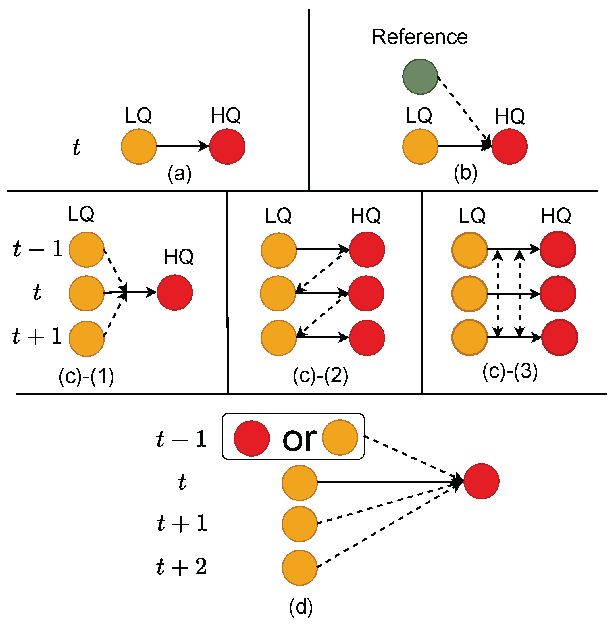
Single-frame-based methods [5,6,7,8,9,10] (Figure 2a) take the current frame as input to reconstruct a sharp image at that time step without using any additional information. Inspired by the physical degradation process, Li et al. [7] jointly learned image reblurring and deblurring in an end-to-end manner, capturing spatially adaptive degradation representations. Chen et al. [6] focused on network simplicity and efficiency by extracting the essential components of state-of-the-art methods and replaced or removed nonlinear activation functions. Single-frame-based methods are simple and efficient, with no cumulative error, but they do not use additional information and are limited in handling complex blur scenarios.
Reference-based methods [12,13,14,15] (Figure 2b) use clear features or structures from reference frames to assist in deblurring the current frame. Liu et al. [12] used the neighboring frames of ground-truth images as reference to assist in restoring blurry images. The results showed that different reference images could significantly affect the clarity of the output. Zou et al. [13] used images captured from different angles, times, or positions as references. The results showed that reference image blur affected the deblurring quality, and the degree of impact depended on the network structure. Li et al. [14] used a ranking correlation module to selectively extract useful features from reference images, improving robustness even when exemplars differed from the input. However, ablation studies showed that removing the correlation module or exemplar had little impact, indicating they did not contribute significantly. Reference-based methods can provide additional information to improve performance, and their effectiveness depends on the quality of the reference frame, which we consider entirely reasonable. However, high-quality reference frames should be easily obtainable without requiring a complex selection process.
Sliding window-based (Figure 2c-(1)), recurrent (Figure 2c-(2)), and parallel (Figure 2c-(3)) methods recover clear frames by fusing information from the current frame and its neighboring frames. Sliding window-based methods [20,21,22,30,31] take multiple consecutive frames as input and perform deblurring. Recurrent methods [16,17,18,32] sequentially propagate latent features or deblurred results from one frame to the next. Parallel methods [23,24] restore all frames in parallel. Due to differences in input and output, these three methods each have their own advantages and disadvantages, as shown in Table 1. Considering the diverse application scenarios of video deblurring, the challenge is to achieve ease of use, feature reuse, rich observational information, minimal error accumulation, support for parallel computation, and high processing speed.
As shown in Figure 2d, to achieve feature reuse, richer information, and improved computational efficiency, we extend sliding window-based methods to include the previously reconstructed frame, the current frame, and future frames. To enable temporal parallel computation, the previously reconstructed frame can be replaced by the previous frame. The remaining challenge is how to mitigate the error accumulation introduced by the previously reconstructed frame while still achieving satisfactory results during parallel computation.

2.2. Temporal Fusion

Sliding window-based methods focus on utilizing information from neighboring frames. Zhang et al. [34] utilized temporal–spatial attention module and frame channel attention module to capture temporal and spatial information from neighboring frames. Zhang et al. [20] utilized a spatio-temporal deformable attention module to capture sharp pixel information from consecutive video frames. Li et al. [35] built a correlation volume pyramid by matching pixels between the reference and neighboring frames. Cao et al. [21] proposed Temporal Transformers to aggregate clear features from neighboring frames and Spatial Transformers to reconstruct high-quality latent frames. Most sliding window-based methods [21,35,36] usually adopt a single-stream structure, which, according to [28], increases interference from irrelevant features in neighboring frames.
Recurrent methods focus on how to utilize and propagate hidden states or the previously reconstructed frame between frames. Zhong et al. [17] propagated hidden information through residual dense blocks and employed a global spatio-temporal attention to fuse temporal features. Ji et al. [18] used a memory bank to store blurry–sharp feature pairs, providing effective information for the propagation and fusion of hidden features in the bidirectional recurrent network. Lin et al. [32] used ConvLSTM [37] to update hidden features while propagating and updating the cell state across time, capturing long-range temporal feature variations. The hidden features were fused with the current frame features via simple element-wise addition. Zhu et al. [16] proposed a simple yet effective multi-scale bi-directional propagation module, designed to capture inter-frame information from unaligned neighboring hidden states across multiple scales, without requiring explicit alignment. Some methods [38,39] used the previously reconstructed frame as the input between frames. The feature processing in these methods is very similar to that of sliding window-based methods. Although recurrent methods inherently cannot perform temporal parallel computation, if the network is designed to allow the previously reconstructed frame to be replaced with an alternative input, the output may be affected but remains usable. In this case, data from different time steps can be processed in parallel, enabling temporal parallel computation.
Parallel methods [23,24] perform long-range feature interactions between frames to improve deblurring effectiveness, resulting in high memory usage.
We observe that some single-frame methods outperform certain methods that exploit neighboring frames. This may be because the latter methods [35,40] do not differentiate the roles of different input frames and instead extract features using the same approach, preventing full utilization of both the current and neighboring frame features.

3. Proposed Methods

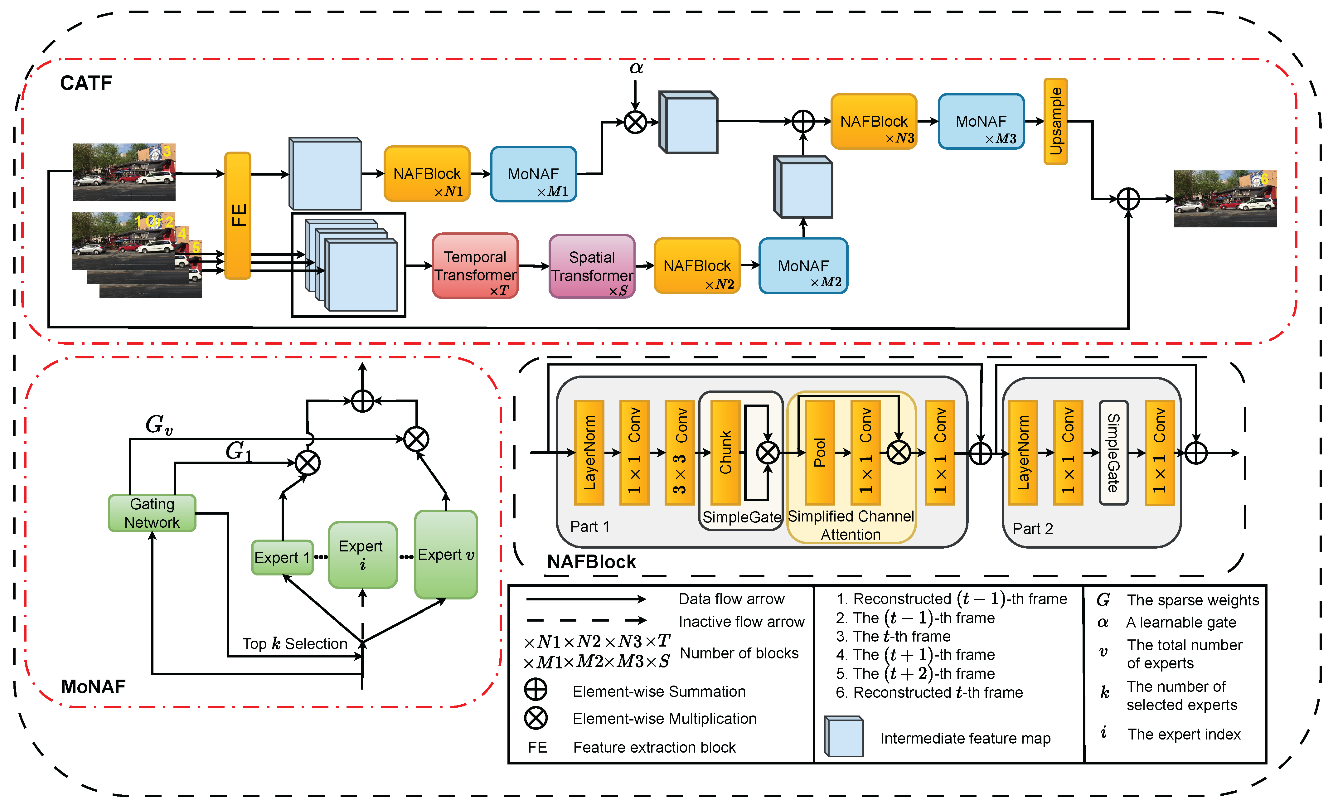
As shown in Figure 3, this paper proposes a Current-Aware Temporal Fusion (CATF) framework, comprising a current-frame reconstruction branch and a neighboring-frame reconstruction branch. The collaborative design of the two branches alleviates interference from irrelevant features in neighboring frames, which is common in single-stream architectures. The features of the current frame are rich and can be directly used for detail reconstruction via convolutional modules, while the features of neighboring frames are first aggregated through Transformer-based modules to extract clear features before detail reconstruction. By employing differentiated feature extraction and a simple fusion strategy, the features of the current frame are fully utilized, with neighboring frame features providing corresponding assistance. Subsequently, we introduce a Mixture-of-Experts module [29] based on NAFBlocks (MoNAF) to adaptively select its structure according to the input, reducing the inference time without compromising the reconstruction quality. Finally, to alleviate the error accumulation arising from temporal sequential dependencies while supporting parallel computation, we adopt a training strategy that preserves the reconstruction quality of temporal sequences and ensures that parallel computation achieves comparably satisfactory results.

3.1. The Current-Aware Temporal Fusion Framework

Transformer and convolution are currently the two most popular network architectures. Multi-Head Self-Attention (MSA) facilitates the integration of global contextual information, whereas convolution excels at modeling local structures and fine details [41]. The CATF framework leverages the complementary strengths of both: for current-frame reconstruction, convolution modules are used to restore local features, while for the reconstruction of a neighboring frame, the Transformer module first integrates the clear features from neighboring frames, followed by convolution modules for local refinement. The input to the CATF framework consists of the previously reconstructed frame R t 1 R 3 × H × W , the current frame F t input R 3 × H × W , and the subsequent two frames F t + 1 input R 3 × H × W and F t + 2 input R 3 × H × W . The output is the reconstructed current frame R t .
First, as shown in Figure 3, R t 1 , F t i n p u t , F t + 1 i n p u t , and F t + 2 i n p u t are fed into the FE block for feature extraction. The FE block consists of three convolutional layers followed by LeakyReLU activations, producing the feature representations R t 1 F E , F t F E , F t + 1 F E , F t + 2 F E R C × H p × W p .
Then, the current frame is independently processed using convolutional modules to extract high-frequency spatial features, where the convolutional modules are implemented as NAFBlocks [6]. The reconstructed feature of the current frame, denoted as F t C , out R C × H p × W p is obtained as follows.
F t C = NAFBlock ( F t F E ) ,
F t C , o u t = MoNAF ( F t C ) ,
where NAFBlock ( · ) represents the NAFBlock, and MoNAF ( · ) is described in Section 3.2.
Next, the reconstruction of a neighboring frame employs a Temporal Transformer to extract clear temporal information from neighboring frames, while a Spatial Transformer captures spatial information for high-quality reconstruction. Subsequently, NAFBlock and the proposed MoNAF are applied to enhance the high-frequency components of the reconstructed frame. The reconstructed feature of a neighboring frame, denoted as F t + 1 N , o u t R C × H p × W p is obtained as follows.
F t + 1 T T = G T T ( C a t ( R t 1 F E , F t + 1 F E , F t + 2 F E ) ) ,
F t + 1 L T = G S T ( F t + 1 T T ) ,
F t + 1 N , o u t = MoNAF ( NAFBlock ( F t + 1 L T ) ) ,
where G T T and G S T denote the Temporal Transformer and the Spatial Transformer [21], respectively.
The main difference between the Temporal and Spatial Transformers lies in how they compute the Query, Key, and Value. In the Temporal Transformer, these are computed as Q T T R ( w × w ) × ( H p w × W p w ) × C , and K T T , V T T R ( w × w × 3 ) × ( H p w × W p w ) × C .
P T T = Flatten ( C a t ( R t 1 F E , F t + 1 F E , F t + 2 F E ) + L P E T T ) ,
Q T T = P t + 1 T T W q T T , K T T = P T T W k T T , V T T = P T T W v T T ,
where H p and W p represent H p and W p , respectively. L P E T T R ( w × w × 3 ) × 1 × C provides a 2D learnable positional encoding to enhance spatial positional information, and Flatten ( · ) converts patches into one-dimensional vectors. P t + 1 T T R ( w × w ) × ( H p w × W p w ) × C denotes the patch from the ( t + 1 ) -th frame used as the Query, indicating that only the features of the ( t + 1 ) -th frame are reconstructed. W q T T , W k T T , W v T T R C × C are learnable linear projection matrices.
In the Spatial Transformer, the Query, Key, and Value are computed as Q S T , K S T , V S T R ( w × w ) × ( H p w × W p w ) × C .
P S T = Flatten ( F t + 1 T T + L P E S T ) ,
Q S T = P S T W q S T , K S T = P S T W k S T , V S T = P S T W v S T ,
where L P E S T R ( w × w ) × 1 × C is the 2D learnable positional encoding, P S T R ( w × w ) × ( H p w × W p w ) × C denotes the input patches, and W q S T , W k S T , W v S T R C × C are the learnable linear projection matrices.
After that, F t + 1 N , o u t is incorporated into F t C , o u t through a simple and efficient fusion strategy, thereby mitigating artifacts introduced by alignment errors.
F t M = F t + 1 N , o u t + α F t C , o u t ,
where α R C × 1 × 1 is a learnable weight.
Finally, we further reconstruct F t R R C × H p × W p from the fused features F t M R C × H p × W p .
F t R = MoNAF ( NAFBlock ( F t M ) ) ,
R t = Upsample ( F t R ) + F t i n p u t ,
where Upsample ( · ) progressively enlarges the feature maps through convolution and PixelShuffle operations.

3.2. The Mixture-of-Experts Module Based on NAFBlocks

Given that the degree of blur may vary across frames in a video, we propose a Mixture-of-Experts module [42] based on NAFBlocks (MoNAF). MoNAF extends the standard NAFBlock by introducing a heterogeneous Mixture-of-Experts mechanism. Each expert is constructed with a different depth, allowing the network to adaptively choose the most suitable one for each input, thereby ensuring both effective and efficient deblurring. As shown in Figure 3, the NAFBlock is divided into Part 1 and Part 2, where Part 2, Part 1, and the full NAFBlock act as shallow, medium, and deep experts, respectively. The function MoNAF ( · ) applied to F t C is defined as follows.
Top-k , i Top-k = TopK ( Gate ( F t C ) , k ) ,
g t , r = Softmax ( Top-k ) r , r = 1 , , k ,
G t , i = g t , r , if i = i Top-k ( r ) for some r , 0 , otherwise , i = 1 , , v ,
F t C , out = i = 1 v G t , i E i ( F t C ) ,
where Gate ( · ) maps F t C to expert logits over v experts. TopK ( · , k ) selects the top-k experts and returns their logits Top-k R 1 × k and their indices i Top-k = ( i Top-k ( 1 ) , , i Top-k ( k ) ) { 1 , , v } k , ordered in the same way as Top-k . The vector g t = ( g t , 1 , , g t , k ) R 1 × k contains the normalized gating weights over these k experts, so that r = 1 k g t , r = 1 . G t R 1 × v denotes the final sparse gating weights, and F t C , out is obtained as the weighted sum of expert outputs. E i ( · ) denotes the i-th expert.

3.3. The Training Strategy

We generate a new training dataset by linearly combining the input blurred frames with the ground truth at different ratios. This new dataset includes frames with varying levels of blur, which are used as the reconstructed previous frame inputs during training. Since the network learns to handle highly blurred frames during training, it can achieve good results during inference even when the previous frame’s reconstruction is of low quality or when the previous frame is used instead of the reconstructed result in parallel computation. The generated dataset is computed as follows.
R ˜ s , t = A t F s , t i n p u t + ( 1 A t ) × G T s , t
where s denotes the s-th video segment, with s { 1 , 2 , , S } , and t denotes the t-th frame within a video segment, with t { 1 , 2 , , T } . A t represents the weight, where a smaller A t corresponds to a lower level of image blur. Within the same video segment, the values of A t { 0.1 , 0.2 , , 0.9 } are uniformly assigned to all frames in a random order.
The training is divided into three stages. In the first stage, covering the first E 1 epochs, a dataset generated by linear combinations is used as the previous-frame reconstruction input, enabling CATF to handle previous-frame reconstructions with varying degrees of blur. In the second stage, the pre-trained network obtained after E 1 epochs generates ground-truth reconstructions, which are used as the new previous-frame reconstruction dataset to enhance the network’s adaptation to sequential temporal computation. In the third stage, the previous-frame reconstruction dataset is updated again at epoch E 2 . Through these three stages, CATF achieves excellent deblurring performance under sequential temporal computation while maintaining good results under parallel temporal computation.

3.4. Loss Function

3.4.1. Reconstruction Loss

The reconstruction loss guides the network to learn the input–output correspondence in pixel space. The calculation is as follows.
L rec = R G T 2 + ϵ ,
where R denotes the reconstructed image, G T denotes the corresponding ground truth, and ϵ = 0.001 is used to stabilize training.

3.4.2. Perceptual Loss

The perceptual loss uses the Mean-Squared Error (MSE) in the VGG [43] feature space to encourage structures, textures, and edges that better match human perception. The calculation is as follows.
L P e r = MSE ( VGG h ( R ) VGG h ( G T ) )
Here, VGG h represents the feature map produced by the h-th layer of the VGG network.

3.4.3. MoE Loss

The MoE loss [42] is used to balance the utilization of each expert. The calculation is as follows.
GTL b i = 1 , G b i > 0 0 , otherwise
L MoE = CV 2 b = 1 B G b i + CV 2 b = 1 B GTL b i
C V 2 denotes the squared coefficient of variation. G b i denotes the gate weight of the b-th batch sample for the i-th expert.
The total loss is computed as follows.
L Total = L rec + λ L Per + γ L MoE ,
where λ = 0.0001 , and γ = 5 .

4. Experimental Results

4.1. Datasets and Setting

Dataset Configurations: This work uses two synthetic video deblurring datasets, DVD [36] and GoPro [44], as well as a real-world video deblurring dataset, BSD [17]. In BSD, different exposure times are set to obtain paired sharp and blurry videos, including 1 ms 8 ms , 2 ms 16 ms , and 3 ms 24 ms . Longer exposure times correspond to higher levels of blur. In the two synthetic datasets, blurry and sharp video pairs are synthesized from high-FPS sequences captured with devices such as the iPhone 6s, GoPro Hero 4 Black, and Canon 7D. In the BSD real-world dataset, Zhong et al. [17] employed a beam splitter system with two synchronized cameras, C1 and C2. The cameras are set to different exposure times to capture real blurry and sharp video pairs. To balance the irradiance between them, a neutral density filter is placed in front of C1. In our experiments, we use the 1 ms 8 ms and 3 ms 24 ms settings to compare the network’s performance on videos with different blur levels. The configurations of the three datasets are summarized in Table 2.
Configurations of Our Proposed Network: The CATF framework is implemented in PyTorch, using an NVIDIA GeForce RTX 4090 GPU on a Windows system. In our experiments, we set N 1 = 5 , N 2 = 5 , N 3 = 25 , M 1 = 1 , M 2 = 1 , M 3 = 1 , T = 1 , S = 3 , C = 256 , p = 4 , w = 4 , v = 3 (one shallow expert, one medium expert, and one deep expert), k = 2 , E 1 = 1000 , and E 2 = 1500 .
Implementation Details: The training details are summarized in Table 3. We adopt the same training strategy as VDTR [21], including the optimizer settings and learning rate schedule. The MoNAF module and its corresponding loss L MoE are excluded from training during the first 1000 epochs and are activated in the subsequent 1000 epochs.

4.2. Comparison with Video Deblurring Methods

STFAN (ICCV2019) [38], EDVR (CVPRW2019) [22], CDVDTSP (CVPR2020) [45], FGST (ICML2022) [46], STDANet (ECCV2022) [20], VDTR (TCSVT2023) [21], LightVID (TCSVT2024) [32], STCT (TIP2024) [24], and ALK-MoE (TCSVT2025) [47] are selected for the comparison experiments. SSIM [48] and PSNR [49] are utilized for quantitative comparison.

4.2.1. Quantitative Comparison

As shown in Table 4, on the DVD test set, the proposed method achieves higher PSNR than most existing methods, with only a slight decrease compared to ALK-MoE. Although the SSIM scores are slightly lower than those of FGST, LightVID, and ALK-MoE, the differences are very small, and the scores are quite close. As shown in Table 5, on the GoPro test set, the proposed method achieves PSNR and SSIM scores that are slightly lower than but still comparable to the state-of-the-art ALK-MoE and higher than those of the other competing methods. As shown in Table 6, on the BSD test set, while the proposed method underperforms ALK-MoE by 0.56 dB in PSNR and 0.0019 in SSIM on the 1 ms 8 ms exposure test set, it exceeds ALK-MoE in SSIM by 0.0081 on the 3 ms 24 ms exposure test set, demonstrating its potential to handle complex scenarios. Table 7 presents the GFLOPs and running time of the five algorithms achieving the best PSNR and SSIM on the DVD and GoPro test sets. Although our method shows slightly lower PSNR and SSIM compared with ALK-MoE, it remains highly efficient, with GFLOPs 18 % lower and the lowest running time among the compared methods.

4.2.2. Qualitative Comparison

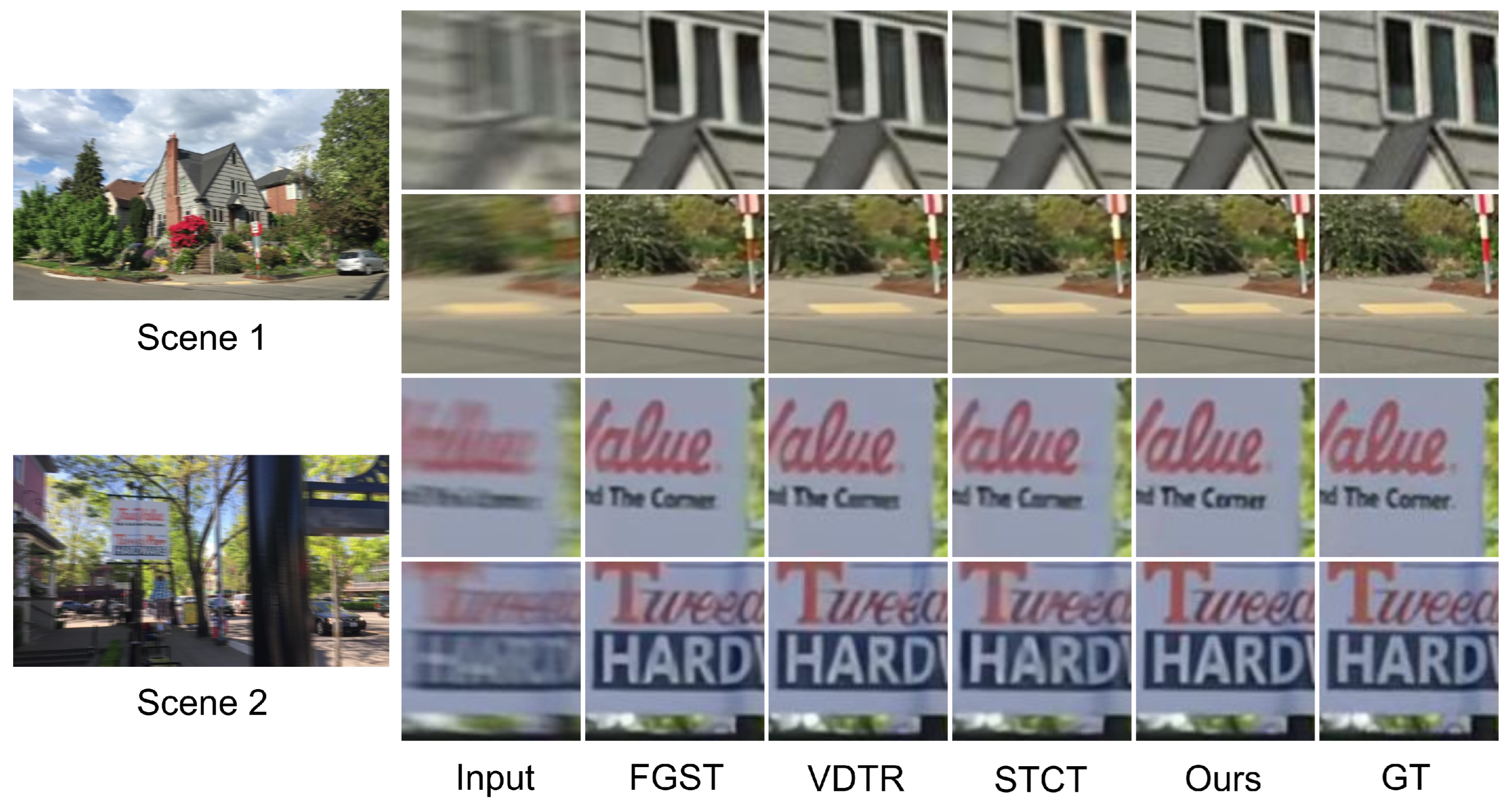
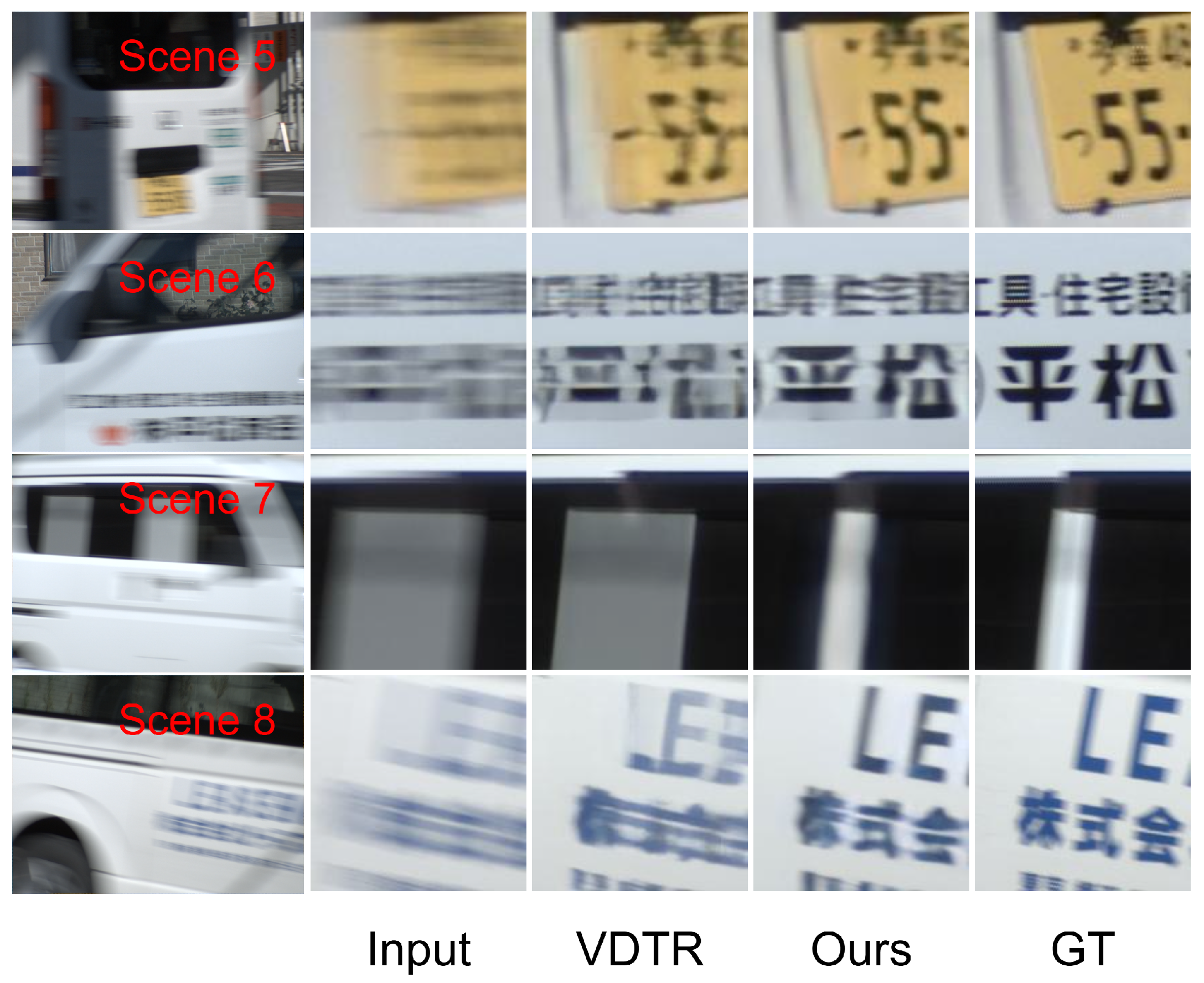
We select algorithms with similar quantitative performance for qualitative comparison: FGST, VDTR, STCT, and ALK-MoE on GoPro and DVD, and VDTR and ALK-MoE on BSD. ALK-MoE is excluded from qualitative evaluation, as it is not open-sourced. Scenes 1 and 2 (Figure 4) are drawn from the DVD test set, Scenes 3 and 4 (Figure 5) from the GoPro test set, Scenes 5 and 6 (Figure 6) from the 1 ms–8 ms exposure test set, and Scenes 7 and 8 (Figure 6) from the 3 ms–24 ms exposure test set. In Scenes 1 and 2, while all methods reconstruct structures well, our method achieves superior performance in detail and contrast. In Scenes 3 and 4, STCT fails to restore structures in extremely blurred regions, likely because its optical flow estimation module does not work well in such areas. VDTR can recover structures but performs poorly on fine details, such as the text in Scene 3. This is because VDTR is Transformer-based, and Transformers mainly aggregate features, while convolutional modules are better suited for high-frequency feature processing. FGST performs well in both structure and detail restoration due to its parallel architecture, which allows the network to utilize long-range feature information. However, FGST aligns and fuses neighboring features via flow guided attention, which causes error accumulation. Therefore, its detail restoration remains less effective than our method. In Scenes 5–8, due to the high relative velocity, VDTR fails to reconstruct fine details and structures, whereas our method succeeds.

4.3. Evaluation of Error Accumulation Mitigation and Parallelism

We design four groups of experiments to verify the ability of our proposed algorithm to suppress error accumulation in temporal dependency inference and its suitability for parallel computation.
Group 1 and Group 2: in the preparation phase, the input at the “previous-frame deblurred result” position is set to either the previous frame, or the GT of the previous frame, to verify whether the algorithm can suppress error accumulation in temporal dependency inference.
Group 3: the previous-frame deblurred result is replaced with the GT of the previous frame throughout all phases, to evaluate the degree of error accumulation in temporal dependency inference.
Group 4: the previous-frame is used throughout all phases, to assess the algorithm’s capability for temporal parallel computation.
As shown in Table 8, in Group 1, the PSNR is only 0.03 dB higher than in Group 2, indicating that the algorithm can adaptively adjust according to the quality of the previous frame’s reconstruction, demonstrating effective mitigation of error accumulation. In Group 3, there is no error accumulation, and compared with Groups 1 and 2, the PSNR increases by only 0.25 dB and 0.22 dB, respectively, indicating that the degree of error accumulation is very small. In Group 4, the PSNR is 0.95 dB lower than Group 1. It still outperforms two methods in Table 5. In PSNR, it is only 0.01 dB below STDANet and 0.12 dB below LightVID, demonstrating the feasibility of parallel computation.

4.4. Ablation Experiment

As shown in Table 9, when the reconstruction of neighboring frames is removed and only the current frame is used for deblurring, the PSNR drops by more than 1 dB compared to CATF. This indicates that the features of both the current frame and neighboring frames are effectively utilized in CATF. Among the three neighboring frames R t 1 , F t + 1 i n p u t , and F t + 2 i n p u t , the reconstruction of F t + 1 i n p u t achieves a PSNR that is 0.08 dB higher than that of R t 1 . This difference is not further investigated in this work, and the results in Table 4, Table 5 and Table 6 are based on the reconstruction of F t + 1 i n p u t .
As shown in Table 10, when using homogeneous experts, each with one Part 1 layer results in lower PSNR and SSIM but achieves faster inference than using two Part 1 layers. With heterogeneous experts adopting different structures, MoNAF achieves higher PSNR and SSIM than homogeneous experts with one Part 1 layer, and faster inference than those with two Part 1 layers. Although MoNAF introduces a modest overhead compared to the plain baseline without MoE, it strikes a better balance between deblurring quality and inference speed, demonstrating the benefit of input-adaptive expert selection.

4.5. Discussion

In this work, we only use PSNR and SSIM for quantitative comparison to remain consistent with prior studies and enable direct comparisons. However, PSNR and SSIM do not always correlate well with human perceptual quality and may not fully reflect improvements in visual appearance. To more comprehensively evaluate the perceptual quality of the restored results, future work will consider incorporating deep learning–based perceptual metrics, such as LPIPS [50] and CLIP-IQA [51].
As shown in Figure 6, CATF performs better than the compared methods in extremely fast motion scenes, but the deblurred results mainly recover coarse structures, and the fine detail reconstruction remains poor. In future work, we will explore event camera based deblurring, and fuse high temporal resolution motion cues with frame images, to improve detail recovery in fast motion scenarios.
Under the 1280 × 720 setting on an NVIDIA RTX 4090, CATF takes 198.8 ms per frame, which corresponds to 5.03 FPS. Under this setting, CATF does not meet real-time requirements. On the BSD dataset, where the input resolution is 640 × 480 , CATF achieves 54.6 ms per frame, which corresponds to 18.31 FPS. Since smooth real-time performance typically requires about 30 FPS, these results indicate that CATF can approach real-time speed when the input resolution is sufficiently small. However, CATF still falls far short of the 240–1000 FPS demanded by high-speed camera applications; so, the current implementation does not yet satisfy such strict real-time constraints. Nevertheless, compared with existing video deblurring methods, CATF achieves a more favorable trade-off between computational cost and deblurring performance.

5. Conclusions

Image sensing tasks are often applied in high-speed scenarios, where the captured images tend to suffer from blur, thereby degrading the sensing accuracy. Based on this, this paper proposes a video deblurring algorithm tailored for image sensing tasks. To achieve high-quality deblurring, fast inference, and wide applicability, this paper proposes a Current-Aware Temporal Fusion with Input-Adaptive Heterogeneous Mixture-of-Experts method. First, single-stream networks are prone to interference from irrelevant neighboring-frame features. The shared extractor cannot fully exploit the distinct cues of the current and neighboring frames. To address this issue, we propose the CATF structure, which employs a dual-stream design and processes the current frame and neighboring frames separately according to the characteristics of convolution and MSA, thereby avoiding interference and fully leveraging the current frame information. Furthermore, considering the large variation in blur across video frames, we design the MoNAF module, which contains heterogeneous experts of varying depths and can select appropriate experts based on the blur level of each frame, thus reducing the inference time while maintaining the deblurring quality. Finally, we propose a training strategy that can both suppress error accumulation under temporally dependent inference and achieve satisfactory results in parallel computation scenarios, thereby enhancing the method’s wide applicability.
We conduct extensive quantitative and qualitative experiments on the DVD, GoPro, and BSD datasets. The quantitative results (Table 4 and Table 5) show that CATF achieves PSNR and SSIM close to those of the latest method ALK-MoE on DVD and GoPro, although slightly lower. On BSD (Table 6), although CATF yields a 0.56 dB lower PSNR than ALK-MoE under the 1 ms–8 ms exposure setting, it achieves higher SSIM under the more challenging 3 ms–24 ms exposure setting, indicating stronger structural fidelity under severe blur. In addition, CATF achieves the shortest average inference time per frame (Table 7), demonstrating a favorable balance between deblurring quality and computational efficiency. Qualitative comparisons (Figure 4, Figure 5 and Figure 6) further confirm that CATF restores image structures and details effectively. Moreover, we validate the feasibility of CATF under both sequential and parallel computation settings (Table 8), and further verify the effectiveness of the CATF architecture and the MoNAF module (Table 9 and Table 10). The results of this paper provide an important supporting technology for image sensing.

Author Contributions

Conceptualization, Y.Z. and A.N.; Methodology, Y.Z. and Z.Z.; Software, Y.Z.; Validation, Y.Z.; Formal analysis, Y.Z.; Investigation, Y.Z.; Resources, Y.Z.; Data curation, Y.Z.; Writing—original draft preparation, Y.Z.; Writing—review and editing, A.N.; Visualization, Y.Z.; Supervision, A.N.; Project administration, A.N.; Funding acquisition, Y.Z. All authors have read and agreed to the published version of the manuscript.

Funding

This work was supported by JST SPRING, Grant Number JPMJSP2109.

Institutional Review Board Statement

Not applicable.

Informed Consent Statement

Not applicable.

Data Availability Statement

Anyone can use or modify the source code for academic purposes only. The code is publicly available at: https://github.com/ZHANGYW1/CATF, accessed on 30 December 2025.

Conflicts of Interest

The authors declare no conflicts of interest.

References

  1. Chang, Y.J.; Hsu, M.C.; Liang, W.Y. Image Sensing for Motorcycle Active Safety Warning System: Using YOLO and Heuristic Weighting Mechanism. Sensors 2025, 25, 7214. [Google Scholar] [CrossRef] [PubMed]
  2. Katsamenis, I.; Bakalos, N.; Lappas, A.; Protopapadakis, E.; Martín-Portugués Montoliu, C.; Doulamis, A.; Doulamis, N.; Rallis, I.; Kalogeras, D. DORIE: Dataset of Road Infrastructure Elements—A Benchmark of YOLO Architectures for Real-Time Patrol Vehicle Monitoring. Sensors 2025, 25, 6653. [Google Scholar] [CrossRef] [PubMed]
  3. Yao, X.; Yuan, H.; Zhao, S.; Tian, W.; Han, D.; Li, X.; Wang, F.; Wang, S. Deep Learning-Based Instance Segmentation of Galloping High-Speed Railway Overhead Contact System Conductors in Video Images. Sensors 2025, 25, 4714. [Google Scholar] [CrossRef] [PubMed]
  4. Xiang, Y.; Zhou, H.; Li, C.; Sun, F.; Li, Z.; Xie, Y. Deep learning in motion deblurring: Current status, benchmarks and future prospects. Vis. Comput. 2025, 41, 3801–3827. [Google Scholar] [CrossRef]
  5. Mao, Y.; Wan, Z.; Dai, Y.; Yu, X. Deep idempotent network for efficient single image blind deblurring. IEEE Trans. Circuits Syst. Video Technol. 2022, 33, 172–185. [Google Scholar] [CrossRef]
  6. Chen, L.; Chu, X.; Zhang, X.; Sun, J. Simple baselines for image restoration. In Proceedings of the European Conference on Computer Vision, Tel Aviv, Israel, 23–27 October 2022; pp. 17–33. [Google Scholar]
  7. Li, D.; Zhang, Y.; Cheung, K.C.; Wang, X.; Qin, H.; Li, H. Learning degradation representations for image deblurring. In Proceedings of the European Conference on Computer Vision, Tel Aviv, Israel, 23–27 October 2022; pp. 736–753. [Google Scholar]
  8. Gong, D.; Yang, J.; Liu, L.; Zhang, Y.; Reid, I.; Shen, C.; van den Hengel, A.; Shi, Q. From Motion Blur to Motion Flow: A Deep Learning Solution for Removing Heterogeneous Motion Blur. In Proceedings of the IEEE Conference on Computer Vision and Pattern Recognition, Honolulu, HI, USA, 21–26 July 2017; pp. 2319–2328. [Google Scholar]
  9. Zamir, S.W.; Arora, A.; Khan, S.; Hayat, M.; Khan, F.S.; Yang, M.H.; Shao, L. Multi-stage progressive image restoration. In Proceedings of the IEEE/CVF Conference on Computer Vision and Pattern Recognition, Nashville, TN, USA, 20–25 June 2021; pp. 14821–14831. [Google Scholar]
  10. Cho, S.J.; Ji, S.W.; Hong, J.P.; Jung, S.W.; Ko, S.J. Rethinking coarse-to-fine approach in single image deblurring. In Proceedings of the IEEE/CVF International Conference on Computer Vision, Montreal, QC, Canada, 10–17 October 2021; pp. 4641–4650. [Google Scholar]
  11. Liu, M.; Yu, Y.; Li, Y.; Ji, Z.; Chen, W.; Peng, Y. Lightweight MIMO-WNet for single image deblurring. Neurocomputing 2023, 516, 106–114. [Google Scholar] [CrossRef]
  12. Liu, C.; Hua, Z.; Li, J. Reference-based dual-task framework for motion deblurring. Vis. Comput. 2024, 40, 137–151. [Google Scholar] [CrossRef]
  13. Zou, H.; Suganuma, M.; Okatani, T. Reference-based motion blur removal: Learning to utilize sharpness in the reference image. arXiv 2023, arXiv:2307.02875. [Google Scholar] [CrossRef]
  14. Li, Y.; Pan, J.; Luo, Y.; Lu, J. Deep ranking exemplar-based dynamic scene deblurring. IEEE Trans. Image Process. 2022, 31, 2245–2256. [Google Scholar] [CrossRef]
  15. Yang, F.; Yang, H.; Fu, J.; Lu, H.; Guo, B. Learning texture transformer network for image super-resolution. In Proceedings of the IEEE/CVF Conference on Computer Vision and Pattern Recognition, Seattle, WA, USA, 13–19 June 2020; pp. 5791–5800. [Google Scholar]
  16. Zhu, C.; Dong, H.; Pan, J.; Liang, B.; Huang, Y.; Fu, L.; Wang, F. Deep recurrent neural network with multi-scale bi-directional propagation for video deblurring. In Proceedings of the AAAI Conference on Artificial Intelligence, Virtual, 22 February–1 March 2022; Volume 36, pp. 3598–3607. [Google Scholar]
  17. Zhong, Z.; Gao, Y.; Zheng, Y.; Zheng, B. Efficient spatio-temporal recurrent neural network for video deblurring. In Proceedings of the European Conference on Computer Vision, Glasgow, UK, 23–28 August 2020; pp. 191–207. [Google Scholar]
  18. Ji, B.; Yao, A. Multi-scale memory-based video deblurring. In Proceedings of the IEEE/CVF Conference on Computer Vision and Pattern Recognition, New Orleans, LA, USA, 18–24 June 2022; pp. 1919–1928. [Google Scholar]
  19. Liu, C.; Wang, X.; Fan, Y.; Li, S.; Qian, X. Decoupling degradations with recurrent network for video restoration in under-display camera. In Proceedings of the AAAI Conference on Artificial Intelligence, Vancouver, BC, Canada, 20–27 February 2024; Volume 38, pp. 3558–3566. [Google Scholar]
  20. Zhang, H.; Xie, H.; Yao, H. Spatio-temporal deformable attention network for video deblurring. In Proceedings of the European Conference on Computer Vision, Tel Aviv, Israel, 23–27 October 2022; pp. 581–596. [Google Scholar]
  21. Cao, M.; Fan, Y.; Zhang, Y.; Wang, J.; Yang, Y. VDTR: Video Deblurring with Transformer. IEEE Trans. Circuits Syst. Video Technol. 2023, 33, 160–171. [Google Scholar] [CrossRef]
  22. Wang, X.; Chan, K.C.; Yu, K.; Dong, C.; Change Loy, C. Edvr: Video restoration with enhanced deformable convolutional networks. In Proceedings of the IEEE/CVF Conference on Computer Vision and Pattern Recognition Workshops, Long Beach, CA, USA, 16-17 June 2019. [Google Scholar]
  23. Liang, J.; Cao, J.; Fan, Y.; Zhang, K.; Ranjan, R.; Li, Y.; Timofte, R.; Van Gool, L. Vrt: A video restoration transformer. IEEE Trans. Image Process. 2024, 33, 2171–2182. [Google Scholar] [CrossRef] [PubMed]
  24. Zhang, L.; Xu, B.; Yang, Z.; Pan, J. Deblurring Videos Using Spatial-Temporal Contextual Transformer with Feature Propagation. IEEE Trans. Image Process. 2024, 33, 6354–6366. [Google Scholar] [CrossRef] [PubMed]
  25. So, J.; Lee, J.; Park, E. Frdiff: Feature reuse for universal training-free acceleration of diffusion models. In Proceedings of the European Conference on Computer Vision, Milan, Italy, 29 September–4 October 2024; pp. 328–344. [Google Scholar]
  26. Boucherit, I.; Kheddar, H. Reinforced Residual Encoder–Decoder Network for Image Denoising via Deeper Encoding and Balanced Skip Connections. Big Data Cogn. Comput. 2025, 9, 82. [Google Scholar] [CrossRef]
  27. Chu, X.; Chen, L.; Chen, C.; Lu, X. Improving image restoration by revisiting global information aggregation. In Proceedings of the European Conference on Computer Vision, Tel Aviv, Israel, 23–27 October 2022; pp. 53–71. [Google Scholar]
  28. Huang, Z.; Chan, Y.L.; Kwong, N.W.; Tsang, S.H.; Lam, K.M.; Ling, W.K. Long short-term fusion by multi-scale distillation for screen content video quality enhancement. IEEE Trans. Circuits Syst. Video Technol. 2025, 35, 7762–7777. [Google Scholar] [CrossRef]
  29. Jacobs, R.A.; Jordan, M.I.; Nowlan, S.J.; Hinton, G.E. Adaptive mixtures of local experts. Neural Comput. 1991, 3, 79–87. [Google Scholar] [CrossRef]
  30. Xiang, X.; Wei, H.; Pan, J. Deep video deblurring using sharpness features from exemplars. IEEE Trans. Image Process. 2020, 29, 8976–8987. [Google Scholar] [CrossRef]
  31. Zhu, Q.; Zheng, N.; Huang, J.; Zhou, M.; Zhang, J.; Zhao, F. Learning spatio-temporal sharpness map for video deblurring. IEEE Trans. Circuits Syst. Video Technol. 2023, 34, 3957–3970. [Google Scholar] [CrossRef]
  32. Lin, L.; Wei, G.; Liu, K.; Feng, W.; Zhao, T. LightViD: Efficient Video Deblurring with Spatial–Temporal Feature Fusion. IEEE Trans. Circuits Syst. Video Technol. 2024, 34, 7430–7439. [Google Scholar] [CrossRef]
  33. Cao, J.; Li, Y.; Zhang, K.; Van Gool, L. Video super-resolution transformer. arXiv 2021, arXiv:2106.06847. [Google Scholar]
  34. Zhang, X.; Wang, T.; Jiang, R.; Zhao, L.; Xu, Y. Multi-attention convolutional neural network for video deblurring. IEEE Trans. Circuits Syst. Video Technol. 2021, 32, 1986–1997. [Google Scholar] [CrossRef]
  35. Li, D.; Xu, C.; Zhang, K.; Yu, X.; Zhong, Y.; Ren, W.; Suominen, H.; Li, H. Arvo: Learning all-range volumetric correspondence for video deblurring. In Proceedings of the IEEE/CVF Conference on Computer Vision and Pattern Recognition, Nashville, TN, USA, 20–25 June 2021; pp. 7721–7731. [Google Scholar]
  36. Su, S.; Delbracio, M.; Wang, J.; Sapiro, G.; Heidrich, W.; Wang, O. Deep Video Deblurring for Hand-Held Cameras. In Proceedings of the 2017 IEEE Conference on Computer Vision and Pattern Recognition, Honolulu, HI, USA, 21–26 July 2017; pp. 237–246. [Google Scholar]
  37. Shi, X.; Chen, Z.; Wang, H.; Yeung, D.Y.; Wong, W.K.; Woo, W.c. Convolutional LSTM network: A machine learning approach for precipitation nowcasting. Adv. Neural Inf. Process. Syst. 2015, 28, 802–810. [Google Scholar]
  38. Zhou, S.; Zhang, J.; Pan, J.; Xie, H.; Zuo, W.; Ren, J. Spatio-temporal filter adaptive network for video deblurring. In Proceedings of the IEEE/CVF International Conference on Computer Vision, Seoul, Republic of Korea, 27 October–2 November 2019; pp. 2482–2491. [Google Scholar]
  39. Son, H.; Lee, J.; Lee, J.; Cho, S.; Lee, S. Recurrent video deblurring with blur-invariant motion estimation and pixel volumes. ACM Trans. Graph. 2021, 40, 1–18. [Google Scholar] [CrossRef]
  40. Xu, Q.; Hu, X.; Luo, D.; Tai, Y.; Wang, C.; Qian, Y. Efficiently exploiting spatially variant knowledge for video deblurring. IEEE Trans. Circuits Syst. Video Technol. 2024, 34, 12581–12593. [Google Scholar] [CrossRef]
  41. Park, N.; Kim, S. How do vision transformers work? arXiv 2022, arXiv:2202.06709. [Google Scholar] [CrossRef]
  42. Shazeer, N.; Mirhoseini, A.; Maziarz, K.; Davis, A.; Le, Q.; Hinton, G.; Dean, J. Outrageously large neural networks: The sparsely-gated mixture-of-experts layer. arXiv 2017, arXiv:1701.06538. [Google Scholar]
  43. Simonyan, K.; Zisserman, A. Very deep convolutional networks for large-scale image recognition. arXiv 2014, arXiv:1409.1556. [Google Scholar]
  44. Nah, S.; Hyun Kim, T.; Mu Lee, K. Deep multi-scale convolutional neural network for dynamic scene deblurring. In Proceedings of the IEEE Conference on Computer Vision and Pattern Recognition, Honolulu, HI, USA, 21–26 July 2017; pp. 3883–3891. [Google Scholar]
  45. Pan, J.; Bai, H.; Tang, J. Cascaded deep video deblurring using temporal sharpness prior. In Proceedings of the IEEE/CVF Conference on Computer Vision and Pattern Recognition, Seattle, WA, USA, 13–19 June 2020; pp. 3043–3051. [Google Scholar]
  46. Lin, J.; Cai, Y.; Hu, X.; Wang, H.; Yan, Y.; Zou, X.; Ding, H.; Zhang, Y.; Timofte, R.; Van Gool, L. Flow-guided sparse transformer for video deblurring. arXiv 2022, arXiv:2201.01893. [Google Scholar] [CrossRef]
  47. Zhang, C.; Xiong, R.; Fan, X.; Zhao, D. Attentive Large Kernel Network With Mixture of Experts for Video Deblurring. IEEE Trans. Circuits Syst. Video Technol. 2025, 35, 5575–5588. [Google Scholar] [CrossRef]
  48. Wang, Z.; Bovik, A.C.; Sheikh, H.R.; Simoncelli, E.P. Image quality assessment: From error visibility to structural similarity. IEEE Trans. Image Process. 2004, 13, 600–612. [Google Scholar] [CrossRef]
  49. Korhonen, J.; You, J. Peak signal-to-noise ratio revisited: Is simple beautiful? In Proceedings of the 2012 Fourth International Workshop on Quality of Multimedia Experience, Melbourne, VIC, Australia, 5–7 July 2012; pp. 37–38. [Google Scholar]
  50. Zhang, R.; Isola, P.; Efros, A.A.; Shechtman, E.; Wang, O. The unreasonable effectiveness of deep features as a perceptual metric. In Proceedings of the IEEE Conference on Computer Vision and Pattern Recognition, Salt Lake City, UT, USA, 18–22 June 2018; pp. 586–595. [Google Scholar]
  51. Wang, J.; Chan, K.C.; Loy, C.C. Exploring clip for assessing the look and feel of images. In Proceedings of the AAAI Conference on Artificial Intelligence, Washington, DC, USA, 7–14 February 2023; pp. 2555–2563. [Google Scholar]
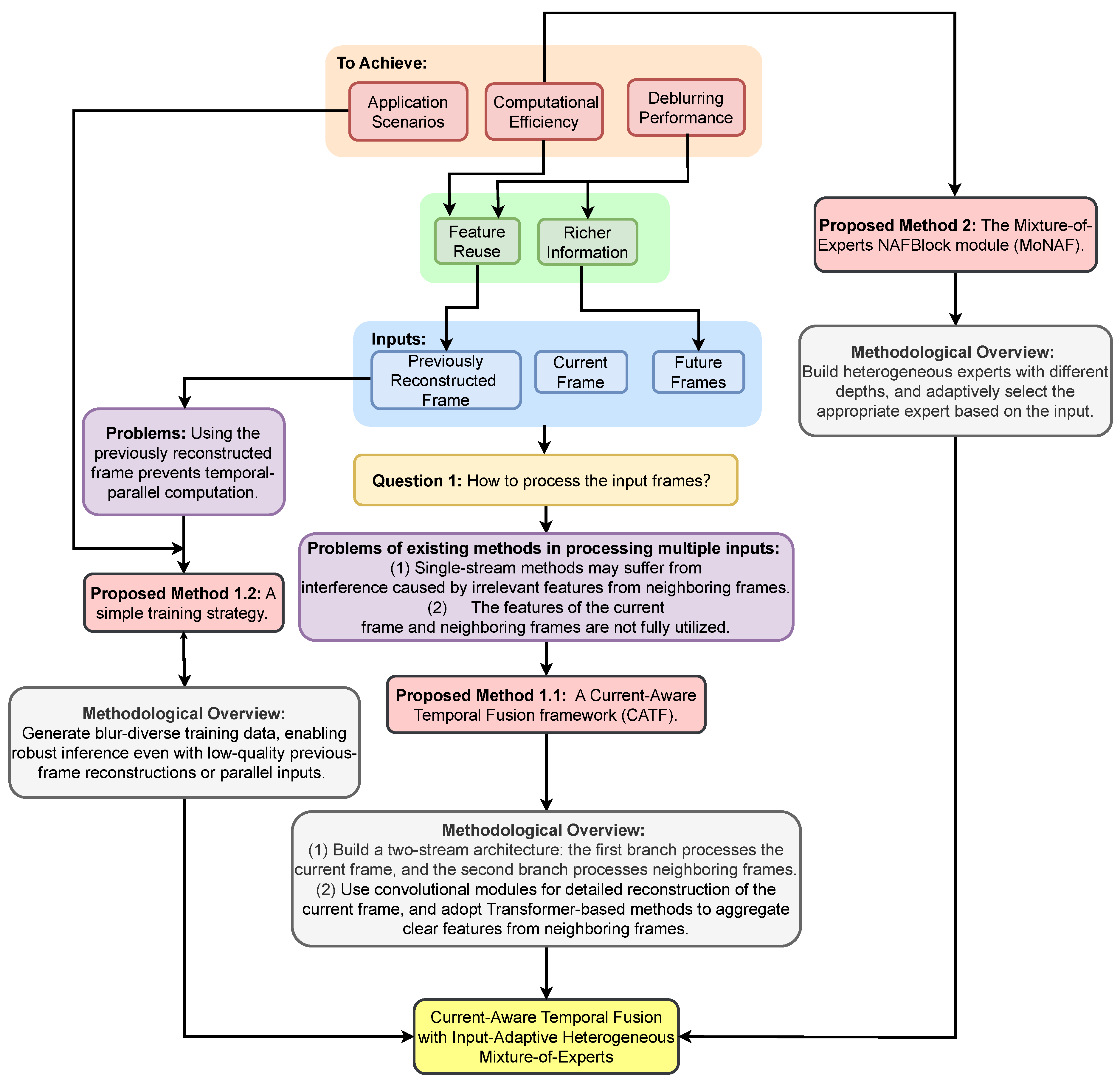
Figure 1. Motivation and design of our method.
Sensors 26 00321 g001
Figure 2. Illustrative comparison of different methods. (a) Single-frame-based method, (b) reference-based method, (c-(1)) sliding window-based method, (c-(2)) recurrent method, (c-(3)) parallel method, and (d) the proposed method. Yellow, red, and green circles denote low-quality input frames, high-quality output frames, and reference frames, respectively. t 1 , t, t + 1 , and t + 2 indicate frame indices. Dashed lines illustrate information fusion across frames. A more detailed explanation is provided in Section 2.1.
Sensors 26 00321 g002
Figure 3. The architecture of the Current-Aware Temporal Fusion (CATF) framework. The CATF and MoNAF (red boxes) are proposed in this paper. CATF corresponds to Equations (1)–(12), and MoNAF corresponds to Equations (13) and (14). The CATF architecture first reconstructs the current frame using a convolutional module composed of NAFBlock and MoNAF, while reconstructing a single neighboring frame with a combination of Temporal Transformer, Spatial Transformer, NAFBlock, and MoNAF. In the Mixture-of-Experts NAFBlock module (MoNAF), the expert structures correspond to the NAFBlock: the deep expert is the complete NAFBlock, the medium expert corresponds to Part 1, and the shallow expert corresponds to Part 2.
Sensors 26 00321 g003
Figure 4. Visual results of DVD test set on different methods.
Sensors 26 00321 g004
Figure 5. Visual results of GoPro test set on different methods.
Sensors 26 00321 g005
Figure 6. Visual results of BSD test set on different methods.
Sensors 26 00321 g006
Table 1. Comparison of video deblurring methods based on different input types.
MethodKey AdvantagesMain Limitations
Sliding Window-BasedFuses temporal information across framesLimits feature reuse across frames;
restricts long-range modeling due to window size
RecurrentShares parameters across frames;
supports feature reuse;
fuses temporal information across frames
Cannot perform parallel computation;
accumulates errors over time; limits long-range modeling;
performs poorly on few-frame videos [33]
ParallelSupports multi-frame parallel processing;
fuses temporal information across frames;
supports feature reuse
Requires a large model;
consumes high memory; constrains scalability by hardware resources
Table 2. The configurations of the three datasets.
DatasetDVDGoProBSD
TrainTestTrainTestTrainValTest
Videos61102211602020
Frames5708100021031111600020003000
Table 3. Training settings.
ComponentSetting
Data augmentationRandom crop (256 × 256), horizontal flips, vertical flips
OptimizerADAM
ADAM parameters β 1 = 0.9 , β 2 = 0.99
Initial learning rate 4 × 10 4 (DVD and GoPro)
2 × 10 4 (BSD)
Epoch2000
Batch size5
Table 4. Evaluations on the DVD test set in terms of PSNR and SSIM. Values from FGST and LightVID are reported to three decimal places. The highest scores are highlighted in bold, while the second-highest scores are indicated with an underline.
MetricSTFANCDVDTSPFGSTSTDANetVDTR
PSNR31.1532.1333.5033.0533.13
SSIM0.90490.92680.9450.93740.9359
MetricLightVIDSTCTALK-MoEOurs
PSNR32.5133.4533.6333.54
SSIM0.9460.94210.94480.9430
Table 5. Evaluations on the GoPro test set in terms of PSNR and SSIM. Values from FGST and LightVID are reported to three decimal places. The highest scores are highlighted in bold, while the second-highest scores are indicated with an underline.
MetricSTFANCDVDTSPFGSTSTDANetVDTR
PSNR28.5931.6733.0232.6233.15
SSIM0.86080.92790.9470.93750.9402
MetricLightVIDSTCTALK-MoEOurs
PSNR32.7332.9733.7933.56
SSIM0.9410.94060.95160.9477
Table 6. Evaluations on the BSD test set in terms of PSNR and SSIM. The highest scores are highlighted in bold, while the second-highest scores are indicated with an underline.
Method1 ms–8 ms3 ms–24 ms
PSNRSSIMPSNRSSIM
STFAN32.780.921929.470.8716
EDVR33.160.932531.930.9261
CDVDTSP33.540.941531.580.9258
VDTR34.120.943632.530.9363
ALK-MoE35.120.950533.420.9372
Ours34.560.948633.090.9453
Table 7. Comparison of model GFLOPs and average per-frame inference time on the GoPro test set (input resolution: 1280 × 720 ). The lowest GFLOPs and the shortest average per-frame inference time are highlighted in bold. The inference time of ALK-MoE is not reported because its code is not publicly available.
MethodGFLOPs (G)Time (ms)
FGST2075.11011.9
VDTR2244.7266.7
STCT44,620.51239.0
ALK-MoE1650.0
Ours1352.1198.8
Table 8. Evaluation of error accumulation mitigation and parallelism on the GoPro test set.
GroupPrevious-Frame
Deblurred Result
(Preparation Phase, 4 Frames)
Replaced with
Previous-Frame
Deblurred Result
(Actual Phase)
Replaced with
PSNRSSIM
Group 1GTDeblurred result33.560.9477
Group 2Previous frameDeblurred result33.530.9475
Group 3GTGT33.780.9492
Group 4Previous framePrevious frame32.610.9378
Table 9. The ablation experiments of the CATF architecture on the GoPro test set in terms of SSIM and PSNR.
MethodPSNRSSIM
CATF (Current-frame reconstruction
and w/o MoNAF)
31.820.9262
CATF (w/o MoNAF)
(Reconstruct R t 1 )
33.110.9432
CATF (w/o MoNAF)
(Reconstruct F t + 1 input )
33.190.9438
Table 10. The MoNAF ablation experiments on the GoPro test set in terms of SSIM and PSNR. “2 Part 1” refers to two layers of Part 1 modules.
TypeThe Numbers of
MoE
Expert 1Expert 2Expert 3PSNRSSIMFPS
NoneNoneNoneNoneNone33.110.94325.40
Homogeneous3Part 1Part 1Part 133.290.94564.77
Homogeneous32 Part 12 Part 12 Part 133.380.94664.56
Heterogeneous3Part 1Part 2NAFBlock33.310.94564.88
Disclaimer/Publisher’s Note: The statements, opinions and data contained in all publications are solely those of the individual author(s) and contributor(s) and not of MDPI and/or the editor(s). MDPI and/or the editor(s) disclaim responsibility for any injury to people or property resulting from any ideas, methods, instructions or products referred to in the content.