
An Accelerated Maximum Flow Algorithm with Prediction Enhancement in Dynamic LEO Networks


Abstract
1. Introduction
- (1)
- We introduce a novel predictive warm-start approach for maximum flow calculations in dynamic LEO networks. The method uses prior and anticipated network states to initialize the algorithm closer to optimal solutions, significantly reducing computation time.
- (2)
- The proposed algorithm incorporates a learning-augmented component that uses historical network patterns to inform flow predictions. This feature allows the algorithm to dynamically adjust to network shifts with minimal recalculations, enhancing its robustness and efficiency in environments with frequent connectivity changes.
- (3)
- We provide a theoretical analysis of the predictive flow algorithm’s feasibility and computational efficiency, supported by extensive empirical validation. Experimental results confirm the algorithm’s robustness and effectiveness across varied network and hardware conditions in LEO environments.
2. Related Work
2.1. TEG and e-TEG in LEO Satellite Networks
2.2. Advancements in Maximum Flow Algorithms
2.3. Software-Defined Satellite Networks
3. System Model and Problem Formulation
3.1. Definitions and Problem Formulation
3.2. Visibility Constraints of Satellite Networks
3.3. Capability Constraints of Satellites
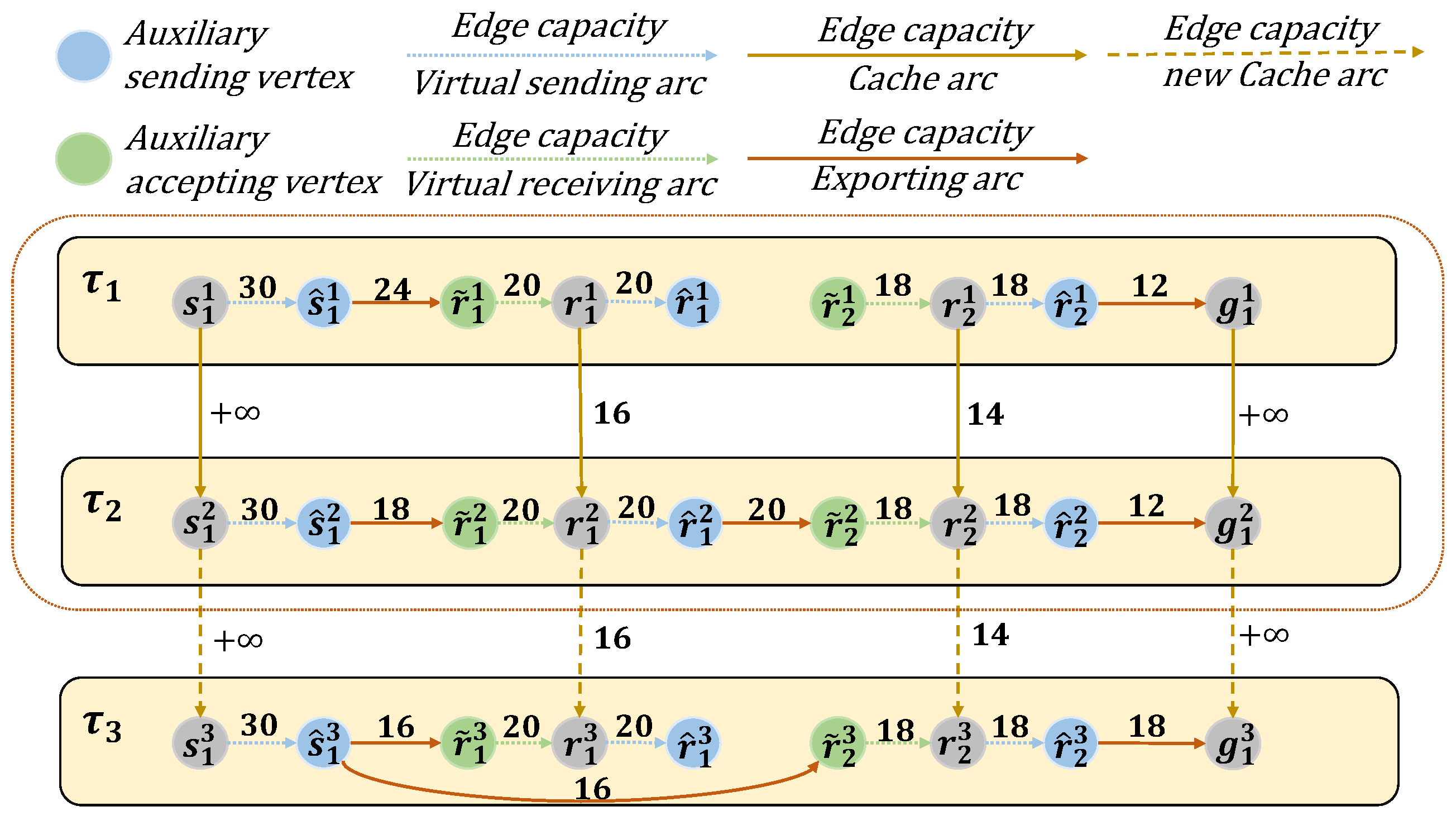
3.4. Construction of the e-TEG Satellite Network
3.5. Update Mechanism of the Residual Network
3.6. Predictive Maximum Flow in e-TEG
3.7. Satellite Network Failures
4. Predictive Acceleration Algorithm for e-TEG Satellite Networks
4.1. Acquisition of Predictive Flow
| Algorithm 1 Acquisition of predictive flow in the e-TEG network. |
|
4.2. Residual Network Update
| Algorithm 2 Residual network update based on the e-TEG network. |
|
4.3. Predictive Accelerated e-TEG Network Maximum Flow Algorithm
| Algorithm 3 Predictive accelerated maximum flow algorithm for e-TEG networks. |
|
|
4.4. SDSN
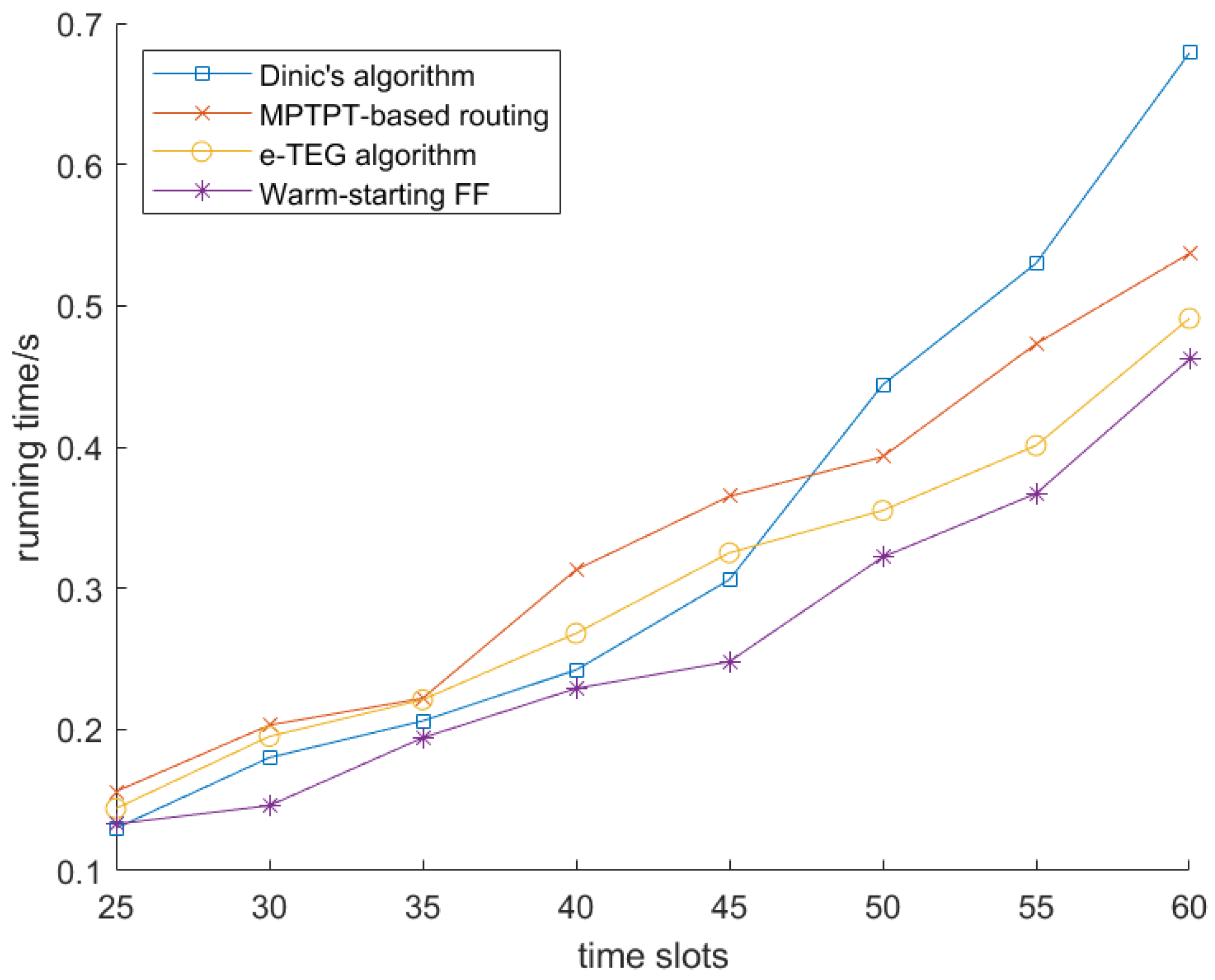
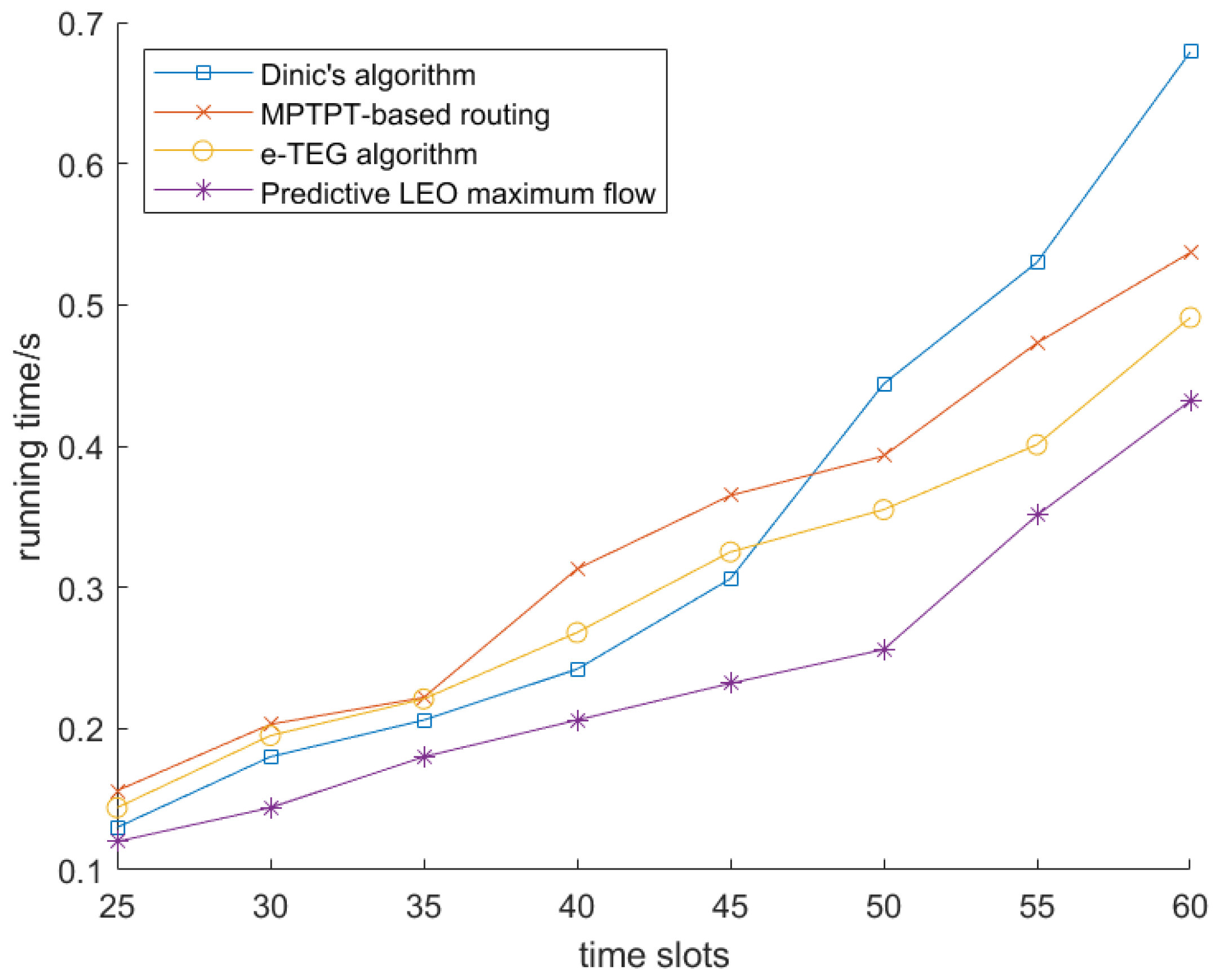
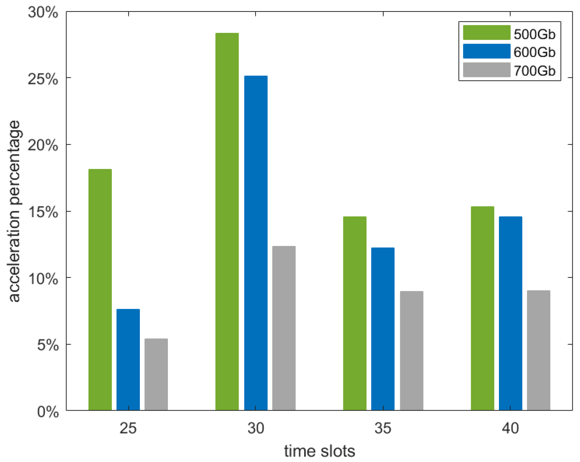
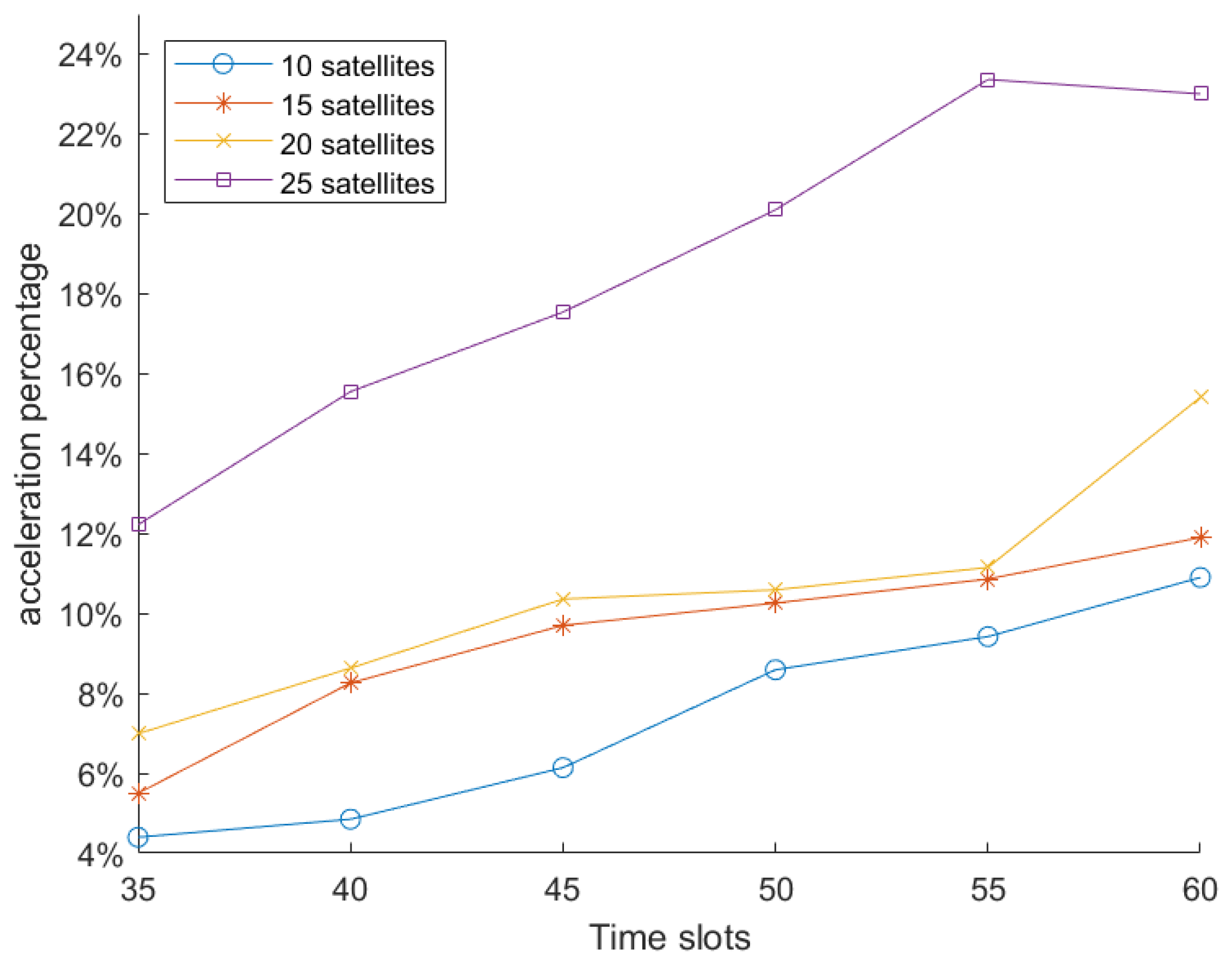
5. Evaluations
6. Conclusions and Future Work
Author Contributions
Funding
Institutional Review Board Statement
Informed Consent Statement
Data Availability Statement
Conflicts of Interest
References
- Foreman, V.L.; Siddiqi, A.; Weck, O.D. Large Satellite Constellation Orbital Debris Impacts: Case Studies of OneWeb and SpaceX Proposals. In Proceedings of the AIAA SPACE and Astronautics Forum and Exposition, Orlando, FL, USA, 12–14 September 2017. [Google Scholar] [CrossRef]
- OneWeb-company. Oneweb constellation. In Proceedings of the 2015 3rd IAPR Asian Conference on Pattern Recognition (ACPR), Kuala Lumpur, Malaysia, 3–6 November 2015.
- Marks, P. Is Amazon Going to Dominate Space? NewScientist 2022, 254, 15. [Google Scholar] [CrossRef]
- Union of Concerned Scientists. UCS Satellite Database. 2024. Available online: https://www.ucs.org/resources/satellite-database (accessed on 8 April 2025).
- Shayea, I.; El-Saleh, A.A.; Ergen, M.; Saoud, B.; Hartani, R.; Turan, D.; Kabbani, A. Integration of 5G, 6G and IoT with Low Earth Orbit (LEO) networks: Opportunity, challenges and future trends. Results Eng. 2024, 23, 102409. [Google Scholar] [CrossRef]
- Lin, H.; Kishk, M.A.; Alouini, M.S. Connectivity of LEO Satellite Mega Constellations: An Application of Percolation Theory on a Sphere. arXiv 2025, arXiv:2502.08019. [Google Scholar] [CrossRef]
- Ford, L.R.; Fulkerson, D.R. Maximal Flow Through a Network. Can. J. Math. 1956, 8, 399–404. [Google Scholar] [CrossRef]
- Dinic, E.A. Algorithm for solution of a problem of maximum flow in networks with power estimation. Sov. Math Dokl. 1970, 11, 1277–1280. [Google Scholar]
- Polak, A.; Zub, M. Learning-augmented maximum flow. Inf. Process. Lett. 2024, 186, 106487. [Google Scholar] [CrossRef]
- Zhu, Y. Intelligent congestion control of data transmission in low Earth orbit satellite networks based on reinforcement learning: Analysis and optimization. Inf. Sci. 2025, 694, 121692. [Google Scholar] [CrossRef]
- Shi, K.; Li, H.; Suo, L. Temporal Graph based Energy-limited Max-flow Routing over Satellite Networks. In Proceedings of the 2021 IFIP Networking Conference (IFIP Networking), Espoo, Finland, 21–24 June 2021; pp. 1–3. [Google Scholar] [CrossRef]
- Kang, Y.; Zhu, Y.; Wang, D.; Han, Z. Efficient Path Selection Design for Large Scale LEO Satellite Constellations Using Graph Embedding-Based Reinforcement Learning. IEEE Trans. Netw. Sci. Eng. 2025, 1–14. [Google Scholar] [CrossRef]
- Wang, P.; Zhang, X.; Zhang, S.; Li, H.; Zhang, T. Time-Expanded Graph-Based Resource Allocation Over the Satellite Networks. IEEE Wirel. Commun. Lett. 2019, 8, 360–363. [Google Scholar] [CrossRef]
- Yang, Y.; Xu, M.; Wang, D.; Wang, Y. Towards Energy-Efficient Routing in Satellite Networks. IEEE J. Sel. Areas Commun. 2016, 34, 3869–3886. [Google Scholar] [CrossRef]
- Lu, C.; Shi, J.; Li, B.; Chen, X. Dynamic resource allocation for low earth orbit satellite networks. Phys. Commun. 2024, 67, 102498. [Google Scholar] [CrossRef]
- Edmonds, J.; Karp, R.M. Theoretical Improvements in Algorithmic Efficiency for Network Flow Problems. J. ACM 1972, 19, 248–264. [Google Scholar] [CrossRef]
- Chen, J.Y.; Silwal, S.; Vakilian, A.; Zhang, F. Faster Fundamental Graph Algorithms via Learned Predictions. arXiv 2022, arXiv:2204.12055. [Google Scholar]
- Sakaue, S.; Oki, T. Discrete-Convex-Analysis-Based Framework for Warm-Starting Algorithms with Predictions. arXiv 2022, arXiv:2205.09961. [Google Scholar]
- Lu, P.; Ren, X.; Sun, E.; Zhang, Y. Generalized Sorting with Predictions. In Proceedings of the SIAM Symposium on Simplicity in Algorithms (SOSA 2021), Virtually, 11–12 January 2021. [Google Scholar]
- Li, C.; Li, H.; Wu, T.; Yan, L.; Cao, S. Realization of maximum flow in DTN and application in CGR. Ad Hoc Netw. 2024, 152, 103302. [Google Scholar] [CrossRef]
- Spridon, D.E.; Deaconu, A.M.; Tayyebi, J. Novel GPU-Based Method for the Generalized Maximum Flow Problem. Computation 2025, 13, 40. [Google Scholar] [CrossRef]
- Gupta, R.; Roughgarden, T. A PAC approach to application-specific algorithm selection. In Proceedings of the 2016 ACM Conference on Innovations in Theoretical Computer Science, Cambridge, MA, USA, 14–17 January 2016; pp. 123–134. [Google Scholar]
- Balcan, M.F.; Deblasio, D.; Dick, T.; Kingsford, C.; Sandholm, T.; Vitercik, E. How much data is sufficient to learn high-performing algorithms? generalization guarantees for data-driven algorithm design. In Proceedings of the Symposium on the Theory of Computing, Rome, Italy, 21–25 June 2021. [Google Scholar]
- Sherman, J. Nearly Maximum Flows in Nearly Linear Time. In Proceedings of the 2013 IEEE 54th Annual Symposium on Foundations of Computer Science, Berkeley, CA, USA, 26–29 October 2013; pp. 263–269. [Google Scholar] [CrossRef]
- Kelner, J.A.; Lee, Y.T.; Orecchia, L.; Sidford, A. An almost-linear-time algorithm for approximate max flow in undirected graphs, and its multicommodity generalizations. In Proceedings of the Twenty-Fifth Annual ACM-SIAM Symposium on Discrete Algorithms, SIAM, Portland, OR, USA, 5–7 January 2014; pp. 217–226. [Google Scholar]
- Chen, L.; Kyng, R.; Liu, Y.P.; Peng, R.; Gutenberg, M.P.; Sachdeva, S. Maximum flow and minimum-cost flow in almost-linear time. In Proceedings of the 2022 IEEE 63rd Annual Symposium on Foundations of Computer Science (FOCS), Denver, CO, USA, 31 October–3 November 2022; pp. 612–623. [Google Scholar]
- Altner, D.; Ergun, Ö. Rapidly solving an online sequence of maximum flow problems with extensions to computing robust minimum cuts. In Integration of AI and OR Techniques in Constraint Programming for Combinatorial Optimization Problems: 5th International Conference, CPAIOR 2008, Paris, France, May 20–23, 2008 Proceedings; Springer: Berlin/Heidelberg, Germany, 2008; pp. 283–287. [Google Scholar]
- Bertaux, L.; Medjiah, S.; Berthou, P.; Abdellatif, S.; Bruyere, M. Software Defined Networking and Virtualization for Broadband Satellite Networks. IEEE Commun. Mag. 2015, 53, 54–60. [Google Scholar] [CrossRef]
- Farris, I.; Taleb, T.; Khettab, Y.; Song, J. A survey on emerging SDN and NFV security mechanisms for IoT systems. IEEE Commun. Surv. Tutor. 2018, 21, 812–837. [Google Scholar] [CrossRef]
- Papa, A.; de Cola, T.; Vizarreta, P.; He, M.; Mas-Machuca, C.; Kellerer, W. Design and Evaluation of Reconfigurable SDN LEO Constellations. IEEE Trans. Netw. Serv. Manag. 2020, 17, 1432–1445. [Google Scholar] [CrossRef]
- Bao, J.; Zhao, B.; Yu, W.; Feng, Z.; Wu, C.; Gong, Z. OpenSAN: A software-defined satellite network architecture. ACM SIGCOMM Comput. Commun. Rev. 2014, 44, 347–348. [Google Scholar] [CrossRef]
- Ayofe, O.A.; Okafor, K.C.; Longe, O.M.; Alabi, C.A.; Tekanyi, A.M.S.; Usman, A.D.; Musa, M.J.; Abdullahi, Z.M.; Agbon, E.E.; Adikpe, A.O.; et al. SDN-Based Integrated Satellite Terrestrial Cyber–Physical Networks with 5G Resilience Infrastructure: Future Trends and Challenges. Technologies 2024, 12, 263. [Google Scholar] [CrossRef]
- Kim, S.; Park, J.; Youn, J.; Ahn, S.; Cho, S. Online Service Function Chain Planning for Satellite–Ground Integrated Networks to Minimize End-to-End (E2E) Delay. Sensors 2024, 24, 7286. [Google Scholar] [CrossRef] [PubMed]
- Salau, A.O.; Beyene, M.M. Software defined networking based network traffic classification using machine learning techniques. Sci. Rep. 2024, 14, 20060. [Google Scholar] [CrossRef] [PubMed]
- Yan, H.; Guo, J.; Wang, X.; Zhang, Y.; Sun, Y. Topology Analysis of Inter-Layer Links for LEO/MEO Double-Layered Satellite Networks. In Space Information Networks; Yu, Q., Ed.; Springer: Singapore, 2018; pp. 145–158. [Google Scholar]
- Wang, P.; Sourav, S.; Li, H.; Chen, B. One Pass is Sufficient: A Solver for Minimizing Data Delivery Time over Time-varying Networks. In Proceedings of the IEEE INFOCOM 2023—IEEE Conference on Computer Communications, New York, NY, USA, 17–20 May 2023; pp. 1–10. [Google Scholar] [CrossRef]
- Du, J.; Jiang, C.; Zhang, H.; Ren, Y.; Guizani, M. Auction Design and Analysis for SDN-Based Traffic Offloading in Hybrid Satellite-Terrestrial Networks. IEEE J. Sel. Areas Commun. 2018, 36, 2202–2217. [Google Scholar] [CrossRef]
- Wei, W.; Fu, L.; Gu, H.; Lu, X.; Liu, L.; Mumtaz, S.; Guizani, M. Iris: Toward Intelligent Reliable Routing for Software-Defined Satellite Networks. IEEE Trans. Commun. 2025, 73, 454–468. [Google Scholar] [CrossRef]
- AGI. Systems Tool Kit (stk). Available online: https://www.agi.com/products/stk (accessed on 8 April 2025).
- Wang, C.; Ren, Z.; Cheng, W.; Zheng, S.; Zhang, H. Time-Expanded Graph-Based Dispersed Computing Policy for LEO Space Satellite Computing. In Proceedings of the 2021 IEEE Wireless Communications and Networking Conference (WCNC), Nanjing, China, 29 March–1 April 2021; pp. 1–6. [Google Scholar] [CrossRef]
- Walker, J. Some circular orbit patterns providing continuous whole earth coverage. J. Br. Interplanet. Soc. 1971, 24, 369–384. [Google Scholar]
- Vallado, D.; Crawford, P. SGP4 orbit determination. In Proceedings of the AIAA/AAS Astrodynamics Specialist Conference and Exhibit, Honolulu, HI, USA, 18–21 August 2008; p. 6770. [Google Scholar]
- Gushchin, A.; Walid, A.; Tang, A. Scalable routing in SDN-enabled networks with consolidated middleboxes. In Proceedings of the 2015 ACM SIGCOMM Workshop on Hot Topics in Middleboxes and Network Function Virtualization, London, UK, 21 August 2015; pp. 55–60. [Google Scholar]

| Method | Characteristics | Advantages | Limitations |
|---|---|---|---|
| TEG [11] | Models the dynamic topology of satellite networks using time-based snapshots. | Captures temporal variation in connectivity; supports time- aware routing. | Ignores energy, processing, or bandwidth constraints. |
| e-TEG [11] | Extends TEG by incorporating energy constraints using virtual arcs. | Addresses energy limitations; enables energy-aware flow optimization. | Increased model complexity; computationally intensive. |
| Ford–Fulkerson Algorithm [7] | Iteratively finds augmenting paths until no residual capacity exists. | Simple; guarantees max flow in integral capacity networks. | Slow for large or dynamic networks; recomputation required after topology changes. |
| Dinic’s algorithm [8] | Uses layered networks and blocking flows for efficient maximum flow computation. | Lower time complexity , suitable for large-scale networks. | Assumes static topology; complex implementation. |
| Learning-augmented maximum flow algorithm [9] | Uses predicted flow values to accelerate computation, leveraging prior knowledge. | Reduces augmentation steps; adapts to recurring flow patterns. | Prediction quality affects stability. |
| 0–1 Min-cost flow algorithm [17] | Solves min-cost flow under binary capacity and cost constraints. | Efficient for highly structured, restricted problems. | Not directly applicable to general or dynamic satellite topologies. |
| Approximate maximum flow algorithm [24,25] | Computes approximate maximum flows for large-scale networks. | Fast computation; scalable to large networks. | Approximation error; less accurate in constrained or real-time settings. |
| Near-linear maximum flow algorithm [26] | Uses data structures and optimization techniques to achieve near-linear complexity. | Theoretically optimal for very large networks. | Assumes static input; lacks support for real-time adaptability. |
| Time Slots | Acceleration Percentage | |
|---|---|---|
| Warm-Starting FF | Predictive LEO Maximum Flow | |
| 25 | 16.67% | 7.64% |
| 30 | 26.15% | 25.13% |
| 35 | 18.55% | 12.22% |
| 40 | 23.13% | 14.55% |
| 45 | 28.62% | 17.54% |
| 50 | 31.51% | 20.10% |
| 55 | 32.24% | 23.36% |
| 60 | 28.00% | 23.00% |
Disclaimer/Publisher’s Note: The statements, opinions and data contained in all publications are solely those of the individual author(s) and contributor(s) and not of MDPI and/or the editor(s). MDPI and/or the editor(s) disclaim responsibility for any injury to people or property resulting from any ideas, methods, instructions or products referred to in the content. |
© 2025 by the authors. Licensee MDPI, Basel, Switzerland. This article is an open access article distributed under the terms and conditions of the Creative Commons Attribution (CC BY) license (https://creativecommons.org/licenses/by/4.0/).
Share and Cite
Sheng, J.; Guan, X.; Yang, F.; Wan, X. An Accelerated Maximum Flow Algorithm with Prediction Enhancement in Dynamic LEO Networks. Sensors 2025, 25, 2555. https://doi.org/10.3390/s25082555
Sheng J, Guan X, Yang F, Wan X. An Accelerated Maximum Flow Algorithm with Prediction Enhancement in Dynamic LEO Networks. Sensors. 2025; 25(8):2555. https://doi.org/10.3390/s25082555
Chicago/Turabian StyleSheng, Jiayin, Xinjie Guan, Fuliang Yang, and Xili Wan. 2025. "An Accelerated Maximum Flow Algorithm with Prediction Enhancement in Dynamic LEO Networks" Sensors 25, no. 8: 2555. https://doi.org/10.3390/s25082555
APA StyleSheng, J., Guan, X., Yang, F., & Wan, X. (2025). An Accelerated Maximum Flow Algorithm with Prediction Enhancement in Dynamic LEO Networks. Sensors, 25(8), 2555. https://doi.org/10.3390/s25082555