1. Introduction
Direction-of-arrival (DOA) estimation has always been an active research area, playing an essential role in numerous applications, such as radar, sonar, and wireless communications [
1,
2,
3,
4,
5,
6]. An important goal of DOA estimation is to accurately locate closely spaced sources in the presence of a low signal-to-noise ratio (SNR), a limited number of available snapshots, and correlations between signals [
3,
7,
8,
9]. A typical model-based method for DOA estimation is multiple signal classification (MUSIC) [
10,
11]. MUSIC leverages the orthogonality between the signal subspace and the noise subspace, and angle estimation is derived by identifying the peaks of the MUSIC pseudo-spectrum evaluated over a predefined grid. As the grid becomes more densely divided, the computational cost grows, demanding significant resources and hindering real-time processing capabilities. The estimation performance significantly degrades under low-SNR conditions or in the presence of highly correlated signals. To overcome these limitations, researchers have developed various enhanced versions of the MUSIC algorithm [
8,
12,
13,
14], such as the Root-MUSIC algorithm. Another typical algorithm is estimation of signal parameters via rotational invariance techniques (ESPRIT). ESPRIT gives the final estimation of signal parameters through eigenvalue decomposition rather than spectral search, making it more computationally efficient than MUSIC [
15,
16,
17,
18]. Besides MUSIC and ESPRIT, there are several other traditional model-based DOA estimation methods [
2,
5,
19,
20,
21,
22]. The Sparse Iterative Covariance-based Estimation (SPICE) method, proposed by P. Stoica et al., is a technique based on sparse estimation and covariance matrix fitting. It improves estimation accuracy through an iterative optimization process, without relying on traditional methods such as grid search or eigenvalue decomposition (EVD). Unlike other sparse estimation methods, SPICE does not require the manual selection of hyperparameters, thus avoiding the complex selection process in traditional approaches. Although SPICE performs well in low-SNR environments, it may still face challenges when dealing with closely spaced signal sources [
22]. The aforementioned methods require the establishment of rigorous mathematical models. When the models do not match, such as array error, the estimation performance will be severely degraded.
Furthermore, the choice of the array structure plays a crucial role in obtaining superior performance. Investigations into the impact of different array geometries on DOA estimation performance have shown that planar arrays provide significantly higher elevation angle estimation accuracy than volumetric arrays [
23]. Planar arrays typically include linear arrays, rectangular arrays, circular arrays, etc. [
2,
19,
24,
25,
26,
27]. In addressing 1D-DOA estimation tasks, the linear array is a frequently used array configuration due to its relatively low computational complexity, making it highly efficient for the experimental testing of various methods [
2]. For 2D-DOA estimation, rectangular arrays offer higher resolution but require greater computational resources and processing power [
28]. The authors in [
29] employed higher-order unitary propagation operators to enhance the spatial sampling accuracy of the signals and effectively avoid the high computational overhead typically associated with traditional methods. For the uniform circular array (UCA), a method based on fourth-order cumulants and beamspace transformation has been proposed in [
30], which can obtain a larger virtual array aperture to enhance the robustness of the algorithm in low-SNR environments and a limited number of snapshots. In addition, M. Boddi et al. [
31] used an iterative method to estimate the DOAs of plane wave signals received by a UCA. This method not only considers mutual coupling effects modeled as gain and phase errors but also transforms the data collected by the UCA into a virtual uniform linear array to enhance the accuracy of DOA estimation. Besides the aforementioned typical arrays, there are also non-circular arrays, such as the L-shaped array used in this study [
28,
29,
32,
33,
34]. Non-circular arrays, with more flexible geometric configurations, account for the irregular spatial arrangement of array elements, which results in better spatial resolution [
33]. The L-shaped array, with its simple and efficient structural characteristics, has been widely applied in various 2D-DOA estimation problems [
1,
35,
36,
37]. Y. Yang et al. [
1] used an inclined projection operator to fill the gaps in the cross-difference co-array of the nested L-shaped array and reconstruct the virtual correlation matrix, which is then used to estimate the 2D-DOA. This operation significantly improves the degrees of freedom and resolution of DOA estimation under underdetermined conditions. G. Lu et al. [
37] used projection approximation subspace tracking to dynamically update the signal subspace and solve the real-time 2D-DOA estimation problem for the L-shaped array by using the ESPRIT algorithm. The algorithm avoids the eigenvalue decomposition of the covariance matrix, thereby significantly reducing computational complexity. The aforementioned studies indicate that the L-shaped array can decompose the 2D-DOA estimation problem into two 1D problems. This decomposition strategy not only enhances estimation performance but also reduces the demand for system resources, making the L-shaped array highly robust in resource-constrained scenarios. Nevertheless, the limitations of these estimation algorithms still pose a risk of error accumulation in practical applications, especially in scenarios with high noise levels or strongly correlated signal sources.
In recent years, machine learning theory has been an active research area and has been applied to various fields. For the problem of DOA estimation, it can be used to learn the complex nonlinear relationship between array data and signal direction by constructing a labeled DOA training dataset. Once the signal features are extracted based on the underlying signal model, no predefined mathematical model is needed for the subsequent estimation process. Moreover, network parameters are automatically optimized during training by using algorithms like Adam. Earlier machine learning methods with high computational efficiency, such as radial basis function and support vector regression, are sensitive to data outliers and rely heavily on the distribution of the training data. Consequently, these methods may struggle to maintain optimal performance in real-world applications, especially when the input data deviate from the assumed distribution or contain significant noise [
38,
39,
40,
41,
42,
43,
44]. Subsequently, researchers have combined the advantages of deep learning and traditional machine learning techniques by designing more efficient and robust network architectures to further improve the accuracy of DOA estimation, such as deep neural network (DNN), convolutional neural network (CNN), and residual–deep convolutional neural network (RDCN) [
45]. These methods maintain good performance even under conditions of limited snapshots and low SNR [
25,
46,
47]. However, deep learning-based methods for DOA estimation still face several challenges, including sensitivity to low SNR and multipath interference, reliance on large volumes of labeled data, limited generalization to varying array configurations, and vulnerability to overfitting in noisy or dynamic signal environments.
To address these issues, recent studies have proposed various strategies from both model design and input representation perspectives. Hassan et al. [
48] introduced a CNN-based approach that directly regresses DOAs from the covariance matrix, demonstrating strong performance under multipath and low-SNR conditions. Similarly, Liu et al. [
49] developed a non-deep learning method based on iterative optimization with semi-unitary constraints, effectively handling multipath association without requiring prior knowledge of the propagation environment. In parallel, other studies have widely adopted the covariance matrix as network input, as it captures second-order statistical information and improves robustness under noise. Tan et al. [
50] proposed a complex-valued CNN with phasor normalization (C-LeDIM-net) which enhances estimation accuracy by explicitly preserving phase features in the input covariance structure. Zhao et al. [
51] designed a deep CNN that maps the covariance matrix into a binary angular domain, significantly improving estimation under conditions of limited snapshots and low SNR. In recent work, several representative methods have been proposed. Lu et al. [
52] proposed a CNN-based improved CAPON algorithm that preserves the blind estimation advantage of Minimum Variance Distortionless Response (MVDR) while effectively reducing estimation error through cyclic noise reduction. Mylonakis et al. [
53] introduced a spatial attention-enhanced CNN combined with transfer learning, achieving robust performance across varying array configurations with minimal retraining effort. These approaches significantly enhance DOA estimation performance in complex scenarios, promoting greater efficiency and broader applicability in real-world deployments.
In this paper, we propose a fusion framework that introduces triple attention mechanisms into deep convolution for 2D-DOA estimation in coherent multipath scenarios. First, we design the input data based on the L-shaped array for the proposed network model, called Triple Attention Deep Convolution Network (TADCN). Subsequently, the proposed TADCN model is used to estimate the DOAs and generate the corresponding angle pairings. Finally, an angle output module is constructed to achieve more accurate 2D-DOA estimation results. The contributions of our work are summarized as follows:
A completely new model, called TADCN, is proposed; it combines deep convolutional neural network (DCN) and the triple attention mechanism (TAM). The TADCN model implements end-to-end optimization, which can automatically adjust its parameters during training. Unlike traditional attention mechanisms, which fail to capture the multi-dimensional dependencies of signals, TADCN can be used to extract valuable spatial features from the raw data. Experimental results show that TADCN demonstrates superior robustness to noise.
We design a new architecture for 2D-DOA estimation by using the L-shaped array configuration. This structure is capable of simultaneously estimating the angle information and achieving automatic pairing. The angle estimation network is used to estimate the azimuth and elevation angles of the signals based on the covariance matrix. The angle matching network is used to pair the estimated azimuth and elevation angles to form the final angle combination. It also demonstrates strong identification capabilities in multipath propagation and multi-source scenarios. Compared with traditional model-based DOA estimation methods, the proposed architecture can automatically learn signal features without relying on extensive prior knowledge. This allows the method to avoid the dependence on complex mathematical models that traditional methods often require.
The performance of the proposed solution is verified over an extensive set of simulated experiments and compared against traditional MUSIC and ESPRIT algorithms, as well as other deep learning methods, in various experimental setups. The experimental results show that the proposed method has superior performance.
The remainder of this paper is organized as follows:
Section 2 introduces the signal model based on the L-shaped array and discusses the signal information contained in the covariance matrix.
Section 3 presents the architecture of the proposed model in detail.
Section 4 introduces the construction and training process of the angle estimation network and the angle matching network. The advantages and disadvantages of the proposed framework are explored and compared with other common methods by using simulated experiments in
Section 5. Finally,
Section 6 concludes the paper.
2. Singal Model
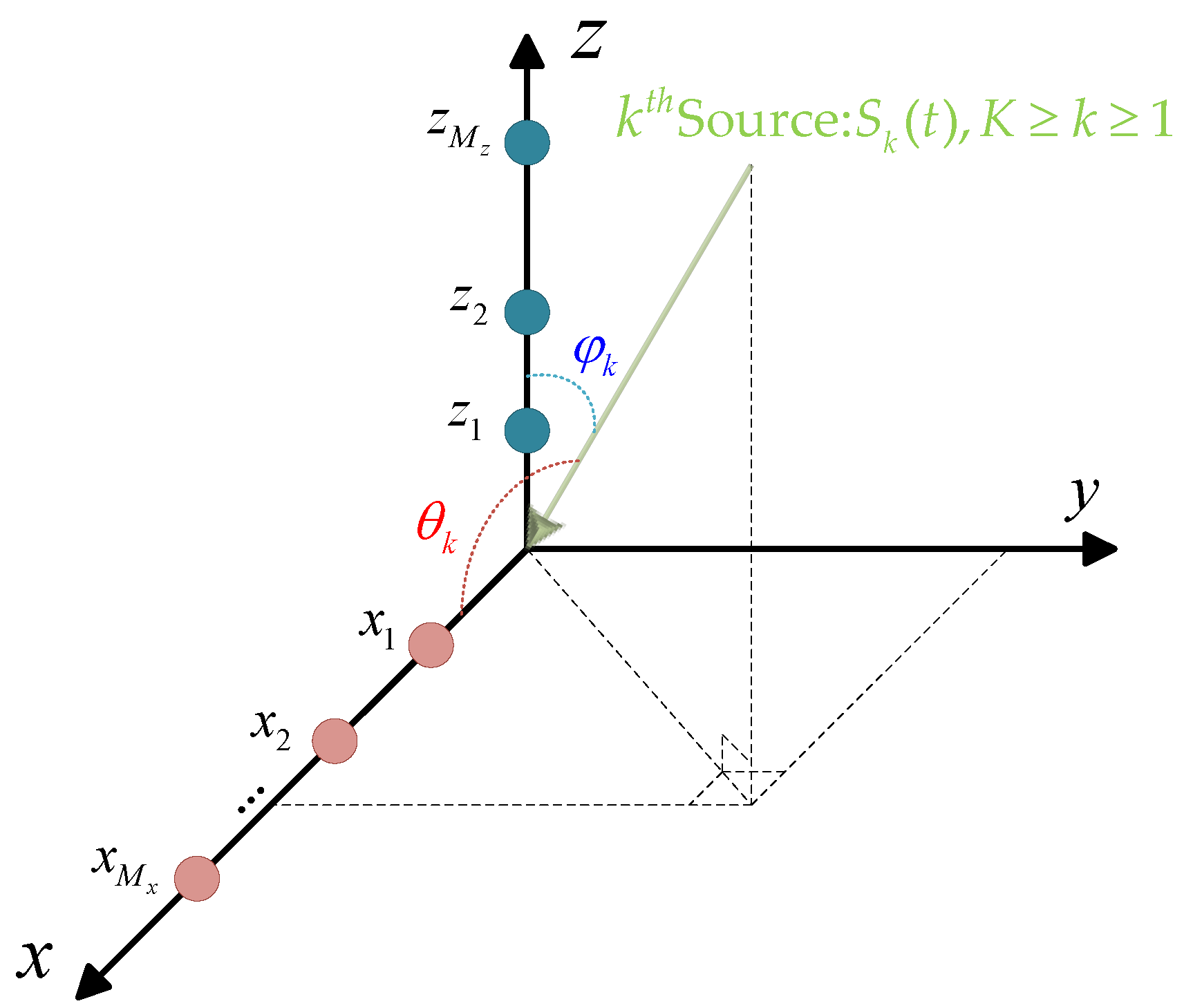
Let us consider an L-shaped array composed of two linear orthogonal arrays, with
and
elements located at positions
and
, respectively, as shown in
Figure 1. We further assume that
narrowband far-field sources are in the surveillance region, impinging on the L-shaped array from
,
, where
represents the angle between the incident direction and the
-axis, while
is the angle relative to the
-axis. Then, the received signals on the L-shaped array in the
-axis and
-axis subarrays are obtained as
where
denotes the random signal received vector.
and
represent the vectors of additive noise of the
-axis and
-axis subarrays, which are temporally and spatially white complex Gaussian with zero mean and variance
and are uncorrelated with incident signals. The matrices
and
are the so-called array manifold matrices, whose
columns contain the angle information from the
source (at location
,
) to the
-axis and
-axis, respectively. Columns
of
, for
, are called steering vectors. We similarly define
of
. The steering vectors of the
source for the
-axis and
-axis subarrays can be represented by
where
is the signal wavelength and
denotes the transpose operation.
From (1), we can see that
is only included in the received data of the
-axis subarray, while
is only included in the received data of the
-axis subarray. So, this representation allows us to exchange the problem of two-dimensional DOA estimation for the problem of two one-dimensional linear array estimations. In addition, it can be seen that
and
have the same structure. To simplify the analysis, we consider only the
-axis subarray for the remainder of this section. In order to improve the performance of DOA estimation, especially at low SNR, we consider the statistics of the received signal. For the
-axis subarray, the covariance matrix
is defined as the second-order statistic of the received signal
:
where
is the conjugate transpose operation and
is the covariance matrix of the signal sources. According to the description of noise in (1), the noise covariance matrix is given by
Therefore, the covariance matrix of the received signal
can be expressed as
In real applications, the ideal covariance matrix is not available, which is estimated by the sample covariance matrix with a finite number of snapshots. We can obtain the estimation of
as follows:
where the estimated values for quantities are expressed as
and
is the number of snapshots. Similarly, the estimation of the covariance matrix for the
-axis subarray can be calculated as
Except for the mappings
and
, there is another very important issue, which is the angular pairing, that needs to be addressed to obtain the knowledge of the location of the sources. Here, we introduce the cross-covariance matrix
, which describes the correlation between the signals of the
-axis and
-axis subarrays, defined as follows:
is used to match
and
to complete two-dimensional DOA estimation. In practice,
is estimated as
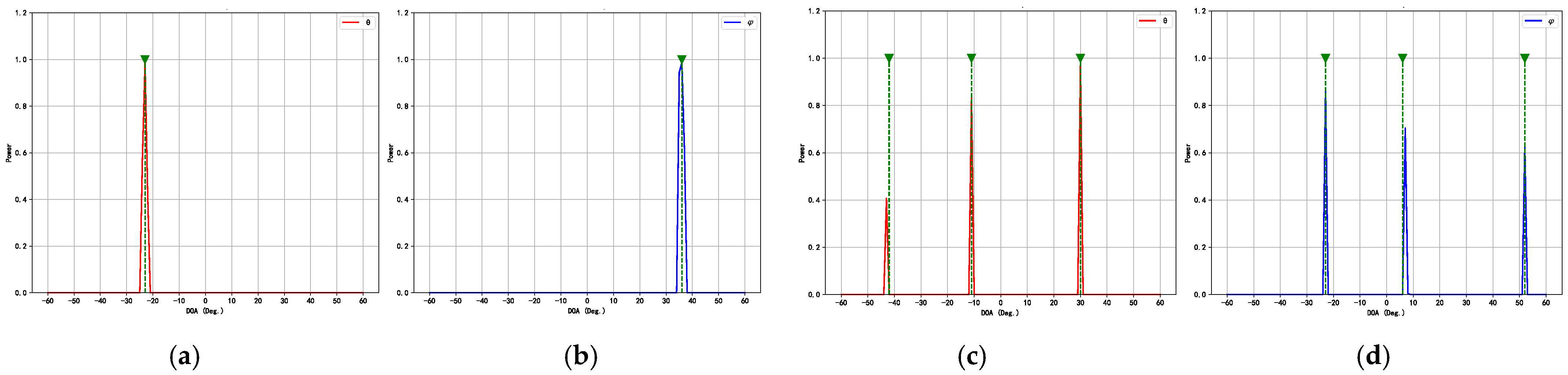
The graphical properties of the cross-covariance matrix
can guide the network in associating
with the correct
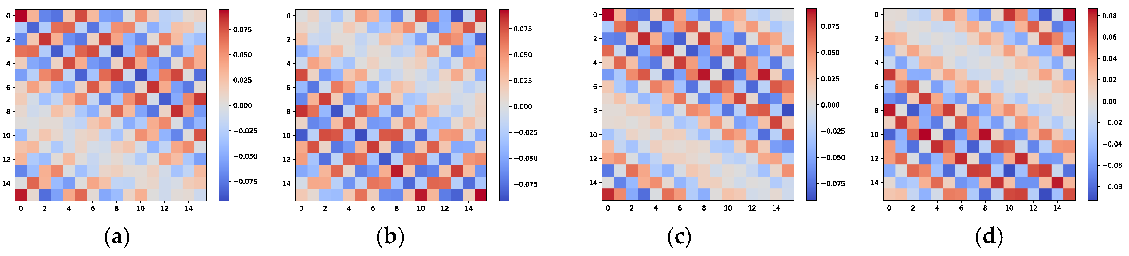
. An example is presented below to demonstrate this. Let us consider an L-shaped array arranged as shown in
Figure 1, where each uniformly spaced linear array includes 16 ideal array elements. Two independent and identically distributed signals,
and
, are present in space, with their azimuth and elevation incident angles taking values in the sets
and
, respectively. According to combinatorial principles,
and
have two possible combinations. The image characteristics of the cross-covariance matrix
corresponding to these two signal arrangements are shown in
Figure 2. To provide a more intuitive visualization of the angular relationships contained in the cross-covariance matrix, we adopt 16 array elements in this illustrative example. It is apparent that the image characteristics of the cross-covariance matrix
for different signal combinations, while similar, exhibit noticeable texture differences, such as in the orientation of the patterns and the positions of larger elements. These differences can be detected by the neural network and incorporated into the parameter matching process.
As explained in the proposed method, we perform 2D-DOA estimation by using , , and .
3. Proposed Method
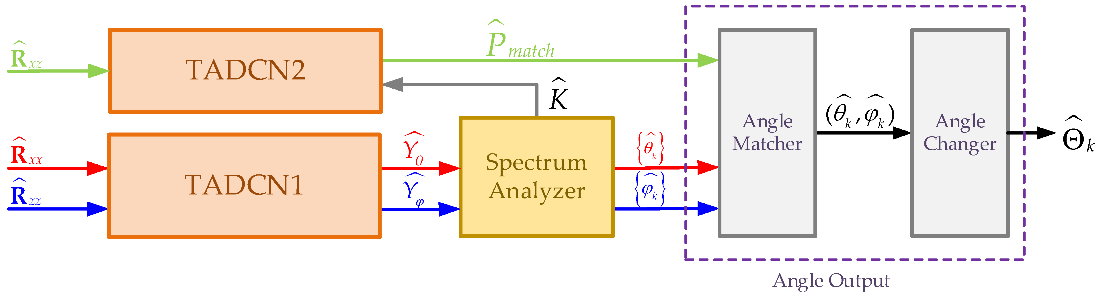
For simplicity, we assume that and that the spacing of the adjacent elements of each subarray is . However, it is important to note that this assumption is made for convenience. The proposed algorithm establishes a mapping between the covariance matrix and DOA and can be applied to any arbitrary L-shaped array, including non-uniform arrays, as long as the covariance matrix can be computed. In this paper, we propose a new TADCN model which is used to train two neural networks: one for DOA estimation and the other for angle combination matching. This process can effectively reduce complexity and improve the accuracy of 2D-DOA estimation. Typically, 2D-DOA estimation requires the network to generate a 2D spatial spectrum. For example, the angle space in and is discretized, which results in the 2D spatial spectrum becoming a matrix of size , where and represent the grid sizes of the angles and , respectively. Such an extensive size of output is hard to deal with. Moreover, the complexity of peak identification within the network is approximately . By using separate networks for angle estimation and matching, the overall complexity is reduced to . The proposed method consists of four consecutive steps, outlined as follows, with detailed descriptions of each step being provided in the subsequent sections:
The estimation covariance matrices and are used as the inputs of the angle estimation network (TADCN1), which outputs the pseudo-spectra and .
The estimation cross-covariance matrix of the received signals from the -axis and -axis subarrays is as the input of the angle matching network (TADCN2), which outputs the probabilities of different angle combinations generated by the possible values of all elements in the sets and .
By using the two pseudo-spectra (, ) from the angle estimation network, the spectrum analyzer module estimates the angle between the incident direction and the -axis , the angle relative to the -axis , and the number of signals .
Finally, the estimated
,
, and angle combinations
from the angle matching network are fed into the angle output module to convert the estimated angles into a suitable form (the azimuth angle and elevation angle) for practical applications (see
Figure 3).
3.1. The Architecture of the Proposed TADCN
As mentioned earlier, the architecture of the proposed method consists of two neural networks for estimation and matching, respectively, which are all based on the proposed TADCN model and different only after the flattening layer. Therefore, we take the angle estimation network (TADCN1) as an example to describe the framework in this section. The proposed TADCN model for DOA estimation is integrated by an innovative combination of triple attention mechanisms (TAMs) and deep convolutional networks (DCNs), which combines the advantages of convolutional layers and multi-dimensional feature interactions to accurately capture the angular characteristics of the signals in the space.
The inputs to the TADCN1 model are the estimation covariance matrices
and
, which are split into the real part and the imaginary part as two channels to facilitate network processing. The overall structure of the TADCN1 model is shown in
Figure 4. There are three network architectures with the same structure, PARTI, PARTII, and PARTIII, to deal with the two channels including comprehensive signal feature information to progressively analyze and extract deeper angle information. As shown in
Figure 4, PARTI consists of a convolutional layer and a TAM layer. After each convolutional layer, a TAM module is added to enhance feature representation. Each layer uses the Leaky ReLU activation function, which is similar to ReLU but outputs a small linear portion when the input is less than or equal to zero. This process is especially useful in deep networks to avoid the ‘dead neuron’ problem. Finally, the features extracted from PARTIII are flattened into a one-dimensional vector which is fed into fully connected layers to reduce the dimensionality gradually and convert the features into an estimated pseudo-spectrum.
3.2. Triple Attention Mechanism
The TAM can be adopted to capture the complex dependencies among the three dimensions of the input tensor: channel (), height (), and width (). Although traditional channel attention mechanisms are computationally efficient and effective, they fail to capture spatial information within feature maps. They only compute scalar weights for each channel (e.g., via global average pooling), resulting in the spatial dimension typically being compressed into a single pixel per channel. In contrast to conventional attention mechanisms, the TAM is a nearly parameter-free attention mechanism that overcomes the limitations of independently computing channel and spatial attention in traditional methods by introducing the concept of cross-dimensional interaction. It captures the dependencies between the channel and spatial dimensions through three parallel branches and effectively compresses the channel dimension while preserving spatial information by using the Z-pool operation. This design not only enhances the ability of the model to integrate multi-dimensional information but also avoids the compression of spatial information in the input tensor. Therefore, the model we used can represent complex features to improve the estimate performance. The TAM, with its efficient and lightweight design, integrates multi-dimensional interactions between channels and spatial information without increasing the computational burden. This makes it possible to use the TAM to extract angular information from features in an efficient manner for DOA estimation tasks in complex signal environments.
The Z-pool operation is one of the key operations in the TAM. To facilitate subsequent lightweight computations while effectively preserving spatial information, Z-pool performs max pooling and average pooling along the zeroth dimension of the input tensor. Then, we concatenate the results along the zeroth dimension. This operation compresses the depth of the original tensor into two dimensions. Mathematically, the Z-pool operation can be expressed as
where
denotes the zeroth dimension. For example, given a tensor
, the output tensor will have the shape
.
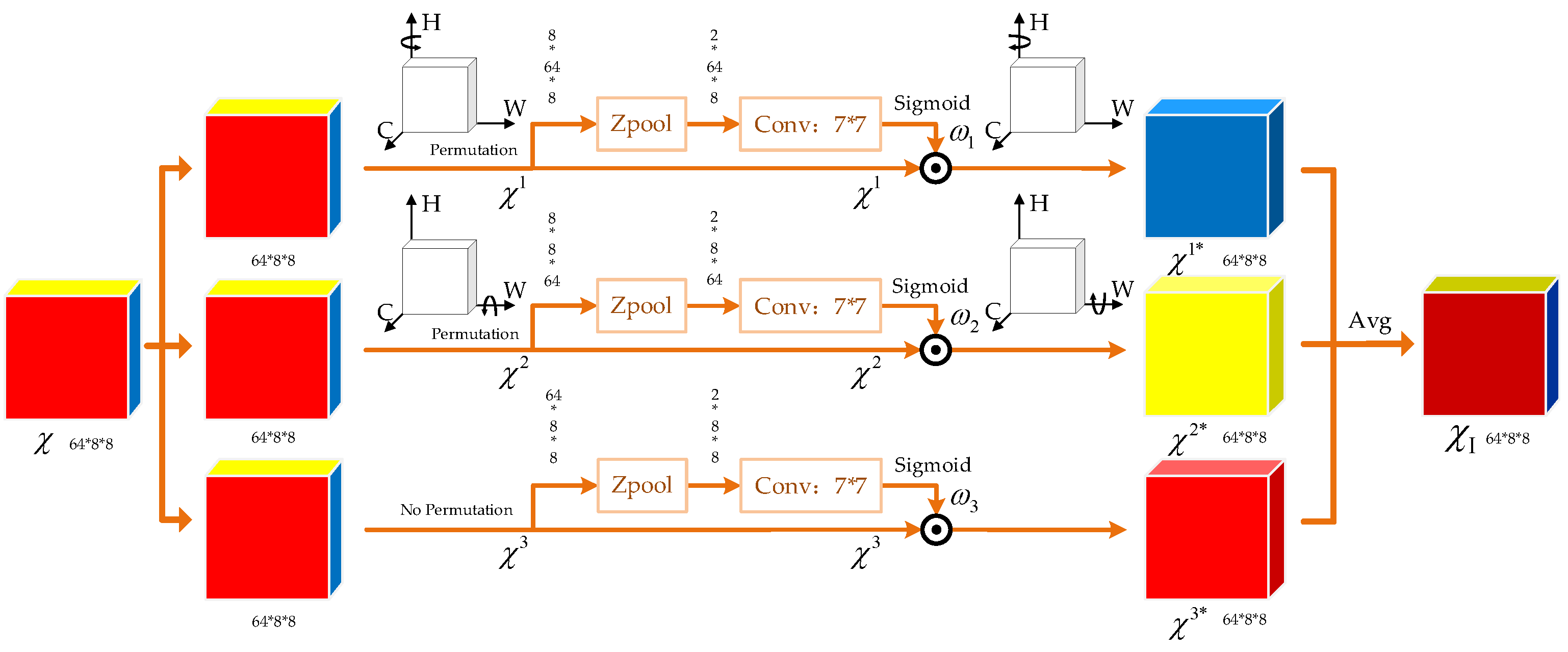
Based on the previously defined operations, the TAM model we use to estimate DOAs consists of three independent attention pathways, each receiving the input tensor and outputting a tensor of the same shape. Every pathway focuses on different dimensional interactions and reconstructs refined feature representations through attention weights. Given an input tensor with C = 64, H = 8, and W = 8, the detailed process is sequentially defined as follows.
In this branch, the input tensor is rotated anticlockwise along the height axis, denoted by , which is used to reconstruct the relationship between the channel and height dimensions. After using the Z-pool operation to compress the width dimension, the tensor undergoes convolution and generates the attention weight multiplied by the rotated tensor . Then, we rotate the multiplication clockwise to ensure that the output tensor has the same dimension as the input tensor, denoted by .
- 2.
Channel–Width Branch
Similarly, the input tensor is rotated along the width axis in this branch, denoted by , which is used to model the dependency between the channel and width dimensions. After the Z-pool operation, the shape of the input tensor becomes and then passes through a convolutional layer with sigmoid activation to generate the attention weight , which is multiplied by . Subsequently, the output of the multiplier is rotated clockwise to restore its original shape, denoted by .
- 3.
Spatial Attention Branch
For the third branch, the Z-pool operation is directly applied to compress the channel dimension to 2, thereby generating attention weight along the spatial dimensions of height and width. The weight is directly multiplied by the input tensor to capture dependencies in the spatial dimensions, denoted by .
The final attention-optimized tensor is obtained by averaging the outputs of the three branches:
The resulting tensor
captures the interdependencies across all three dimensions, enabling a more comprehensive feature representation. This TAM module that makes multi-dimensional interactions possible is essential to improving performance in DOA estimation tasks. The processing flow of the TAM after receiving
is shown in
Figure 5.
3.3. Spectrum Analyzer
In the proposed method, we analyze the spatial spectrum from TADCN1 and employ an angle estimation technique based on linear interpolation to obtain precise estimation results. First, a copy of the original spatial spectrum
is constructed as
, where the values at the indexes of the main peaks with
are set to zero. This operation is performed to suppress the influence of the main peaks on the search for the secondary peaks and to facilitate an accurate search for the position of the secondary peaks within a small range near the main peaks. The position of the secondary peak
is determined by identifying the maximum value within the local region surrounding the main peak index
, specifically in the range from
to
. Formula (12) gives the index of the secondary peak
:
where
denotes the index of the maximum value within a subinterval around the main peak
. Since the search range is localized relative to the main peak (i.e., within the interval
), the returned index corresponds to a local index. The adjustment
is added to convert this into a position in the global spatial spectrum. Upon determining the indices of the main and secondary peaks, the corresponding amplitudes are recorded. The amplitude of the main peak is denoted by
, and the amplitude of the secondary peak is
. By using these amplitudes, the contribution weights of each peak to the final angle estimate are calculated. Specifically, the contribution weights
and
for the main and secondary peaks are computed as follows:
where
and
represent the relative contributions of the main and secondary peaks to angle estimation. Given that the contributions of the main and secondary peaks are unequal, these weight coefficients effectively reflect the relative influence of each peak. The final angle estimate is obtained by computing the weighted average of the main and secondary peak indices. Precisely, the angle estimate
is calculated as follows:
The adjustment term accounts for the offset in the angle range. Unlike traditional methods that rely solely on the main peak, the proposed spectrum analyzer reduces quantization errors by employing the weighted linear interpolation approach using both peaks. This operation will provide greater stability and accuracy, particularly in scenarios with peak overlap or significant noise interference.
3.4. Angle Output
The angle output module of the proposed method comprises two components: the angle matcher and the angle changer. The angle matcher is used to perform angle matching, and the angle changer converts the incident directions relative to the
-axis and
-axis into azimuth and elevation angles. The values
and
derived from the spectrum analyzer is entered into the angle matching network, which outputs the most probable angle pair to provide the final 2D-DOA estimation. For
, the specific procedure is described in Algorithm 1.
| Algorithm 1: Angle matching process. |
- Inputs:
- Output:
Construct possible angle combinations: Select the optimal combination:
|
In practical applications, however, to more accurately describe the DOA of the signal, it is necessary to define the azimuth
as the angle between the incident direction of signal and its projection onto the z–y plane and the elevation
as the angle between the incident direction of signal and its projection onto the x–y plane. This angle can be derived as follows:
Upon completing these tasks, the angle changer outputs , facilitating the subsequent signal angle localization.
4. Data Generation and Network Training
The configuration of the antenna array and the TADCN model have been described in detail earlier. Here, we focus on data generation and network training. A diverse dataset is generated based on random source positions to train the angle estimation network and the angle matching network. For the subsequent simulation experiments, it is assumed that each sample contains two signal sources, i.e., . The incident angles of the signals are randomly selected with the angle range defined as [−60°, 60°]. This angle range is chosen based on practical application scenarios. It effectively covers the spatial region observable by the L-shaped array and avoids the edge degradation commonly observed near detection boundaries. The grid scale is chosen as 1°, resulting in a total of 121 discrete angle values to balance computational efficiency and estimation accuracy. This generation scheme allows the training data to cover the entire spatial domain. The SNR is randomly selected within the range dB, and the number of snapshots is set to . According to the sample design rules outlined above, 50,000 samples were generated randomly, and the dataset is split into training and test sets in a 0.8:0.2 ratio.
We employ the Adam optimizer with a fixed learning rate of 0.0012. At the end of each epoch, the loss trend is recorded to track learning progress and convergence. The training process of the TADCN model for angle estimation and matching is detailed in Algorithm 2, where
,
, and
denote the initial models for
,
, and angle matching processes before any optimization. The symbol
represents the loss function used to train the models in the estimation and matching tasks. The batch size during training is denoted by
B.
and
represent the number of epochs used for training the models related to DOA estimation and the angle matching process, respectively. The binary cross-entropy loss (BCELoss) function is used to quantify the discrepancy between predicted probabilities and true labels. The mathematical expression for BCELoss is given as
where
is the true label,
is the predicted value, and
is the number of samples.
| Algorithm 2: Training process for DOA estimation and angle matching. |
- Inputs
- Outputs
do do Optimizer Adam.step() Optimizer Adam.zero_grad() of size B do Optimizer Adam.step() Optimizer Adam.zero_grad() do of size B do Optimizer Adam.step() Optimizer Adam.zero_grad()
|
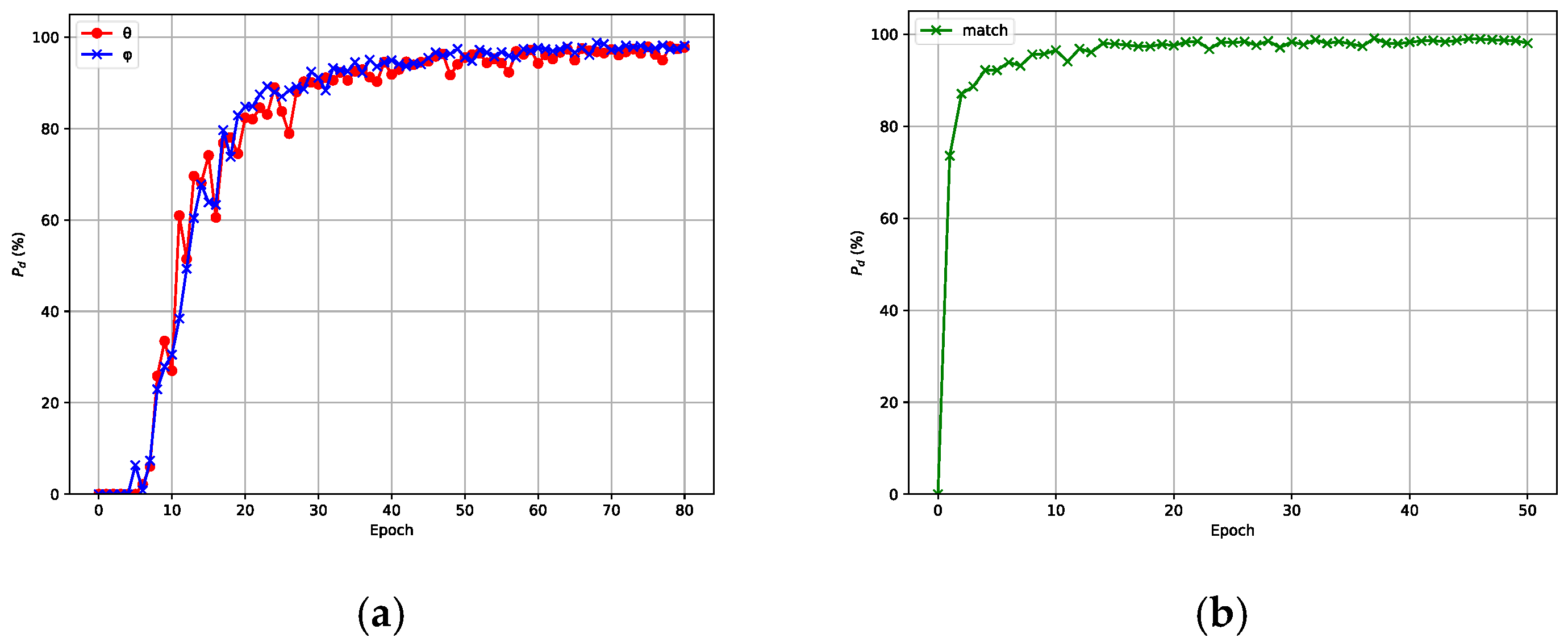
By definition, the two signals are estimated accurately in a single trial if the absolute estimation error for both angles is no more than
. The accuracy
is defined as
where
,
is the number of successful estimation samples, and
is the total number of test samples. The accuracy curve of the model with respect to the number of training iterations is shown in
Figure 6, where (a) corresponds to the angle estimation network and (b) corresponds to the angle matching network. From
Figure 6, we can see that the accuracy will not increase very much when the epoch number reaches a certain value. Considering the training cost and overall performance, the number of epochs for the angle estimation network was designed as 70, while the number of epochs for the angle matching network was set to 45.
Table 1 shows the network structures of the angle estimation and matching networks trained under the aforementioned parameter settings and procedures.


 ,
, 


