Segmented Estimation of Road Adhesion Coefficient Based on Multimodal Vehicle Dynamics Fusion in a Large Steering Angle Range


Abstract
1. Introduction
2. Vehicle Dynamics Modeling
2.1. Tire Model
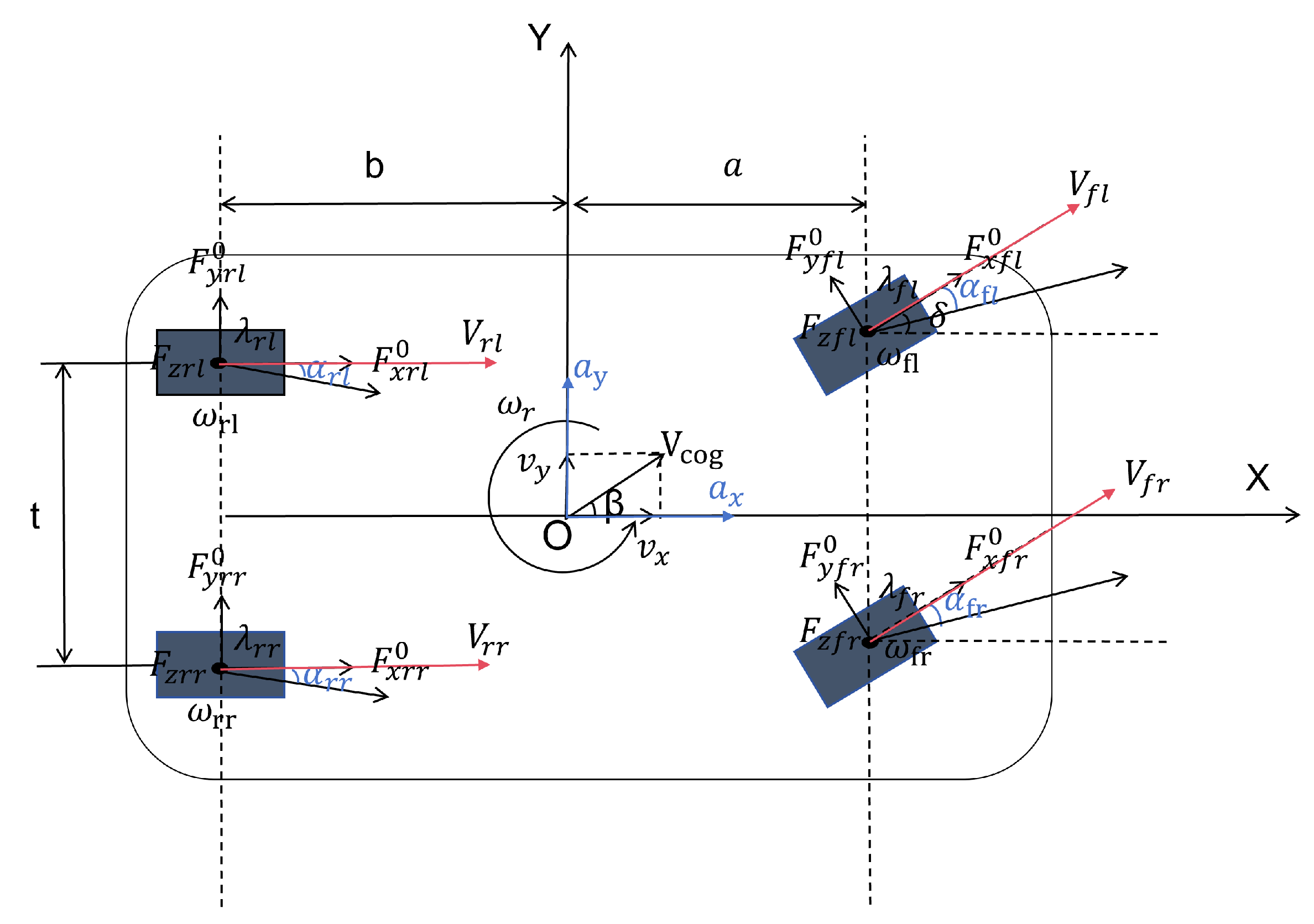
2.2. Vehicle Model
3. Piecewise Combination Estimation of Road Surface Friction Coefficient Based on Dynamics Model Fusion
3.1. Principle of Adaptive Unscented Kalman Filtering
Basic Process of AUKF (Adaptive Unscented Kalman Filter)
3.2. Road Surface Friction Coefficient Estimation Based on Adaptive Unscented Kalman Filtering
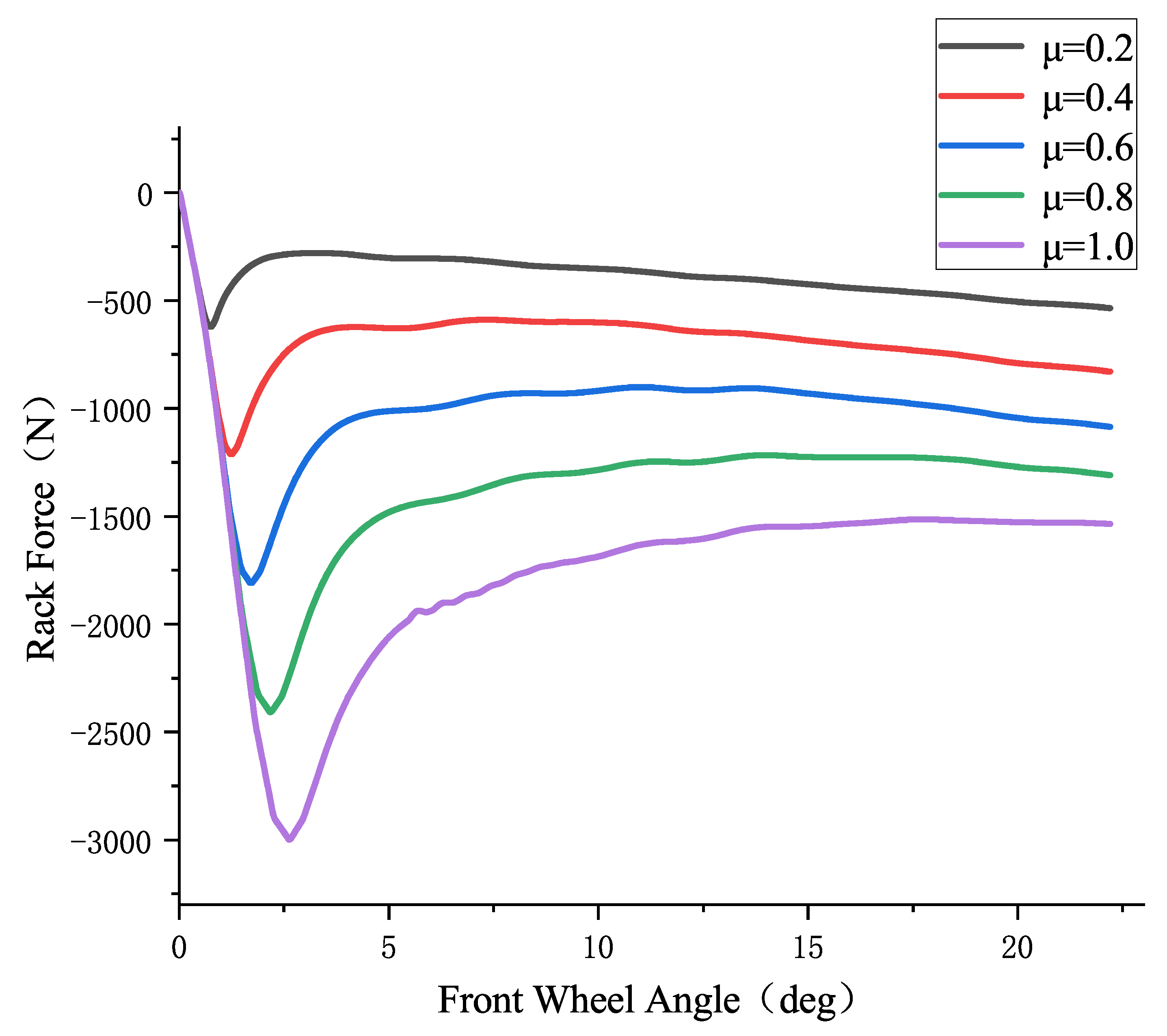
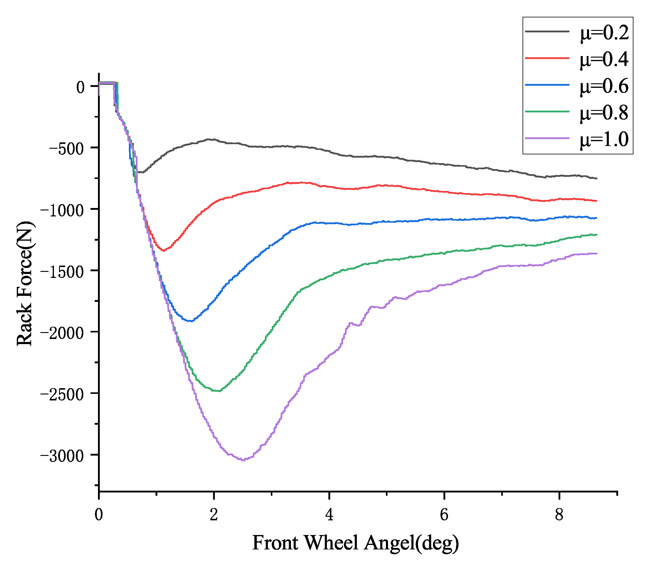
3.3. Road Surface Friction Coefficient Estimation Based on Steering Rack Force
3.3.1. Steering Rack Force Observer Design
3.3.2. Road Surface Friction Coefficient Estimation Based on Steering Rack Force
4. Simulation Experiment and Results Analysis
4.1. Estimation of Road Surface Friction Coefficient Based on the Combination of AUKF Algorithm and Rack Force Method
4.1.1. Joint Simulation of CarSim and Matlab/Simulink
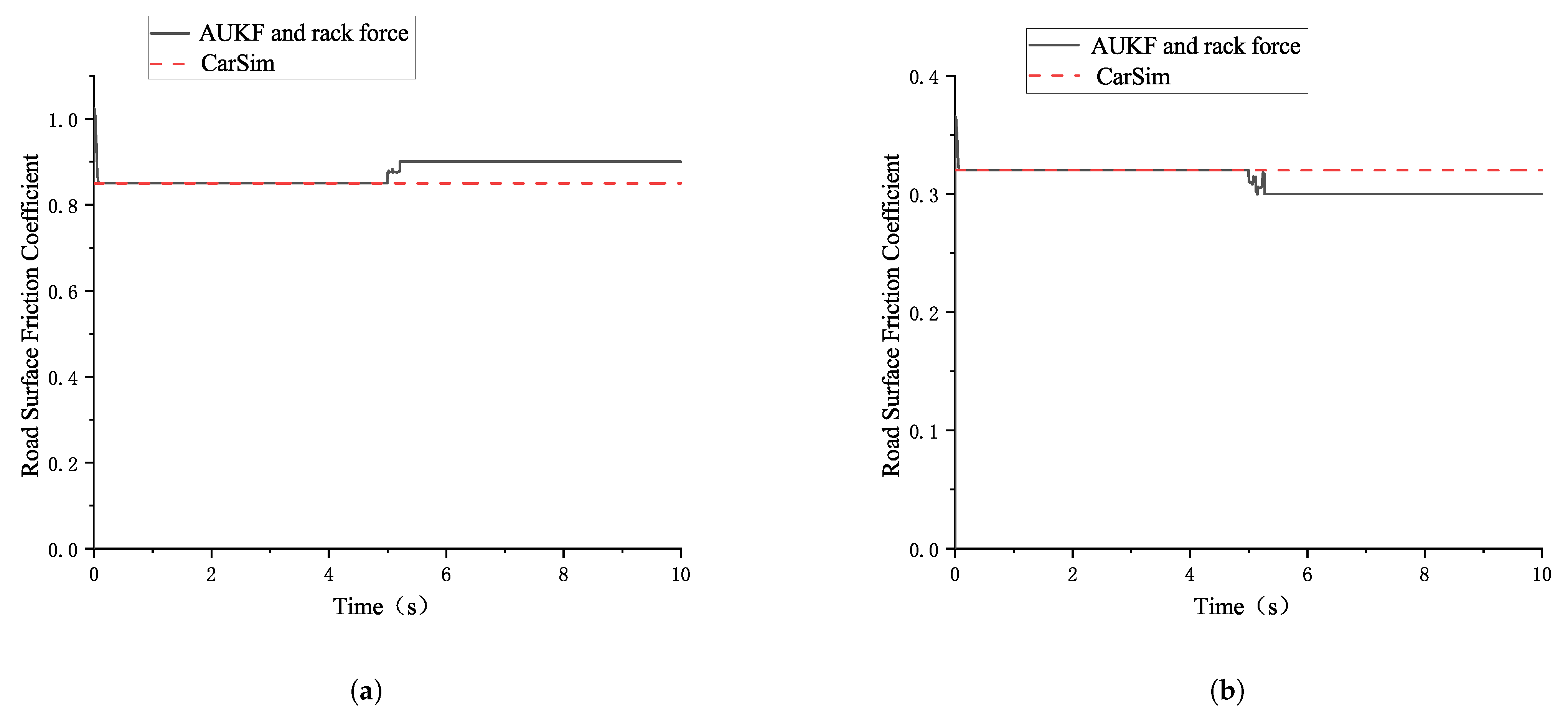
4.1.2. Results Analysis
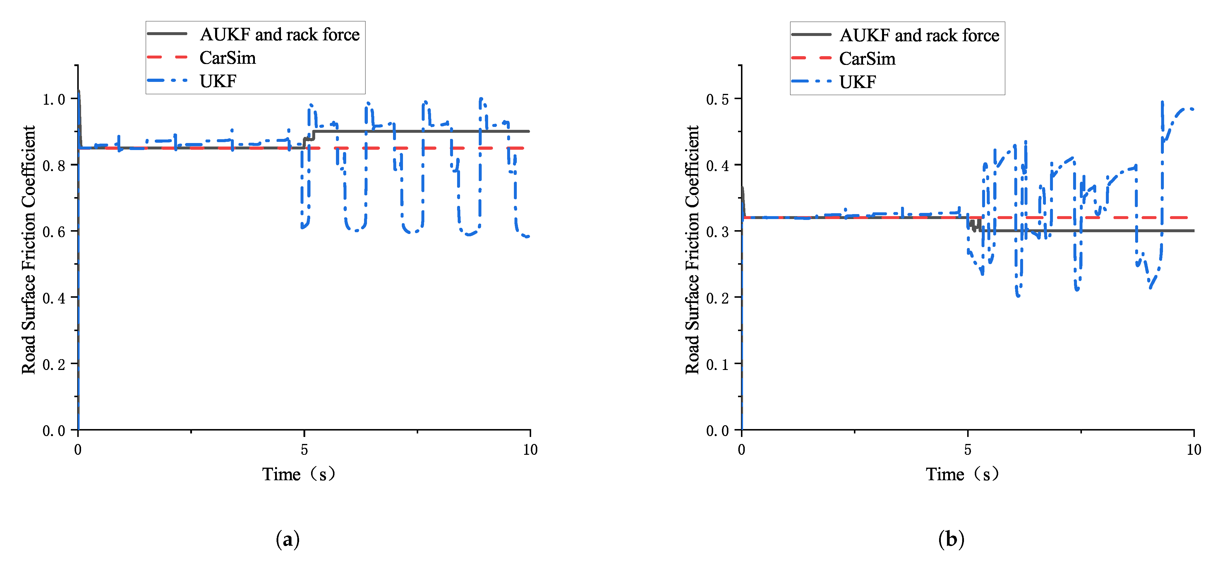
4.2. Comparison with the Unscented Kalman Filter Method Results
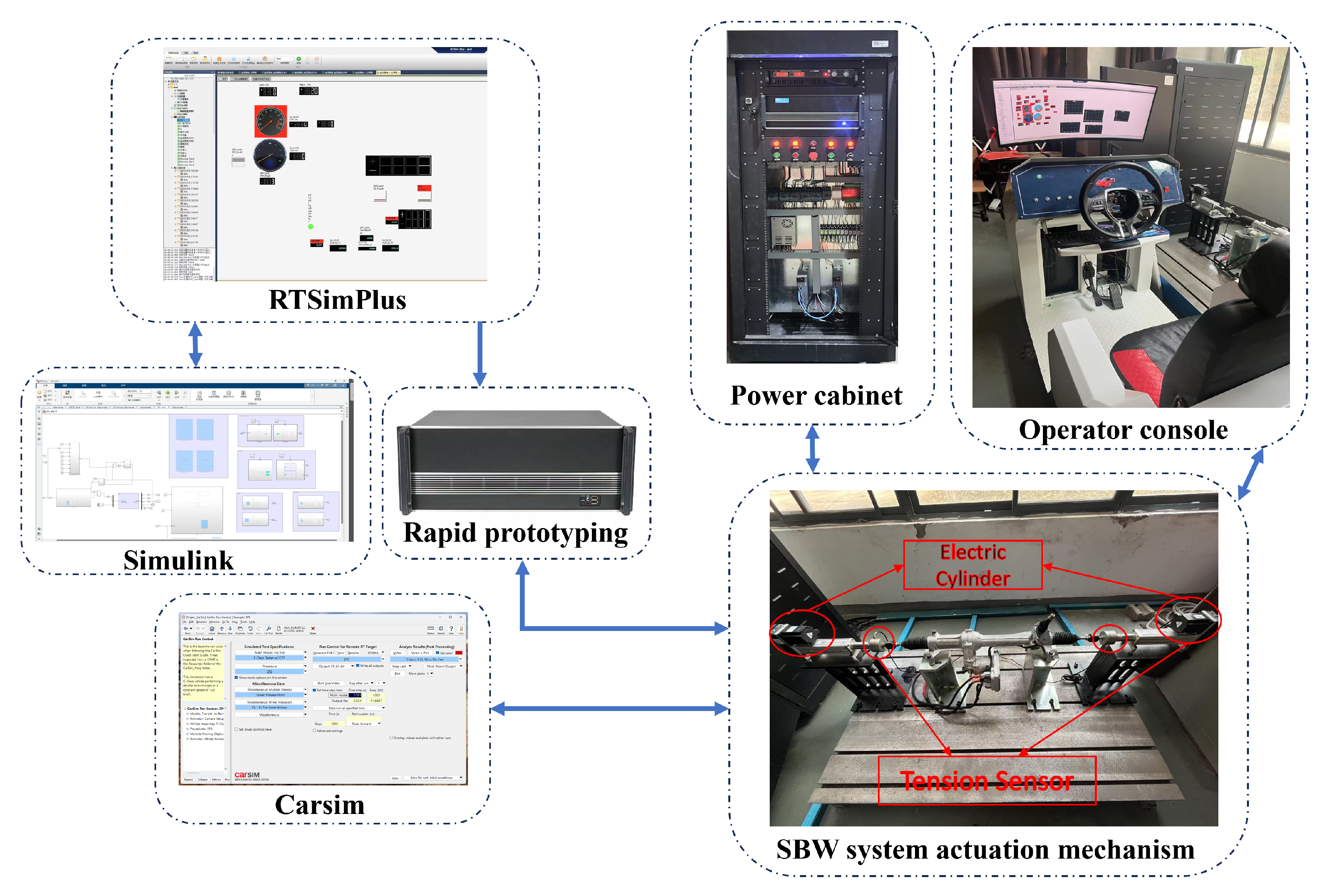
5. HIL Testing of the Steer-by-Wire System
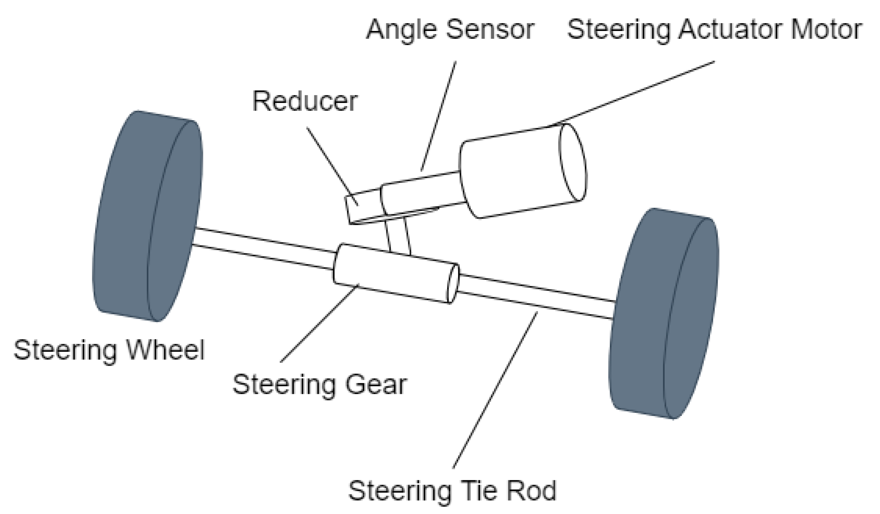
5.1. Composition and Functions of the Steer-by-Wire System HIL Test Rig
5.2. HIL Test of Road Surface Friction Coefficient Estimation Based on AUKF Algorithm and Rack Force Method
5.3. HIL Test Bench Comparison of the Dynamic Fusion Method and the Unscented Kalman Filter Algorithm Estimation Results
6. Conclusions
Author Contributions
Funding
Institutional Review Board Statement
Informed Consent Statement
Data Availability Statement
Conflicts of Interest
References
- Kanafi, M.M.; Kuosmanen, A.; Pellinen, T.K.; Tuononen, A.J. Macro- and micro-texture evolution of road pavements and correlation with friction. Int. J. Pavement Eng. 2015, 16, 168–179. [Google Scholar] [CrossRef]
- Langstrand, J.P.; Randem, H.O.; Thunem, H.; Hoffmann, M. Using Deep Learning to classify road surface conditions and to estimate the coefficient of friction. In Proceedings of the 2023 IEEE Intelligent Vehicles Symposium (IV), Anchorage, AK, USA, 4–7 June 2023; IEEE: Piscataway, NJ, USA, 2023; pp. 1–8. [Google Scholar]
- Otoofi, M.; Laine, L.; Henderson, L.; Midgley, W.J.B.; Justham, L.; Fleming, J. FrictionSegNet: Simultaneous Semantic Segmentation and Friction Estimation Using Hierarchical Latent Variable Models. IEEE Trans. Intell. Transp. Syst. 2024, 25, 19785–19795. [Google Scholar]
- Yan, Z.; Yue, L.; Luo, W.; Sun, J. Real-time detection of road surface friction coefficient: A new framework integrating diffusion model and Transformer in Transformer algorithms. Alex. Eng. J. 2025, 113, 620–632. [Google Scholar]
- Yu, M.; Liu, S.; You, Z.; Yang, Z.; Li, J.; Yang, L.; Chen, G. A prediction model of the friction coefficient of asphalt pavement considering traffic volume and road surface characteristics. Int. J. Pavement Eng. 2023, 24, 2160451. [Google Scholar]
- Jung, D. Experimental Validation of Artificial Neural Network based Road Condition Classifier and its Complementation. IEEE Access 2023, 11, 82696–82708. [Google Scholar]
- Tian, C.; Leng, B.; Hou, X.; Xiong, L.; Huang, C. Multi-sensor fusion based estimation of tire-road peak adhesion coefficient considering model uncertainty. Remote Sens. 2022, 14, 5583. [Google Scholar] [CrossRef]
- Du, Y.; Liu, C.; Song, Y.; Li, Y.; Shen, Y. Rapid estimation of road friction for anti-skid autonomous driving. IEEE Trans. Intell. Transp. Syst. 2019, 21, 2461–2470. [Google Scholar]
- Leng, B.; Jin, D.; Xiong, L.; Yang, X.; Yu, Z. Estimation of tire-road peak adhesion coefficient for intelligent electric vehicles based on camera and tire dynamics information fusion. Mech. Syst. Signal Process. 2021, 150, 107275. [Google Scholar]
- Singh, K.B.; Ali Arat, M.; Taheri, S. An intelligent tire based tire-road friction estimation technique and adaptive wheel slip controller for antilock brake system. J. Dyn. Syst. Meas. Control 2013, 135, 031002. [Google Scholar]
- Lampe, N.; Ziaukas, Z.; Westerkamp, C.; Jacob, H.G. Analysis of the potential of onboard vehicle sensors for model-based maximum friction coefficient estimation. In Proceedings of the 2023 American Control Conference (ACC), San Diego, CA, USA, 31 May–2 June 2023; IEEE: Piscataway, NJ, USA, 2023; pp. 1622–1628. [Google Scholar]
- Schäfke, H.; Lampe, N.; Kortmann, K.P. Transformer Neural Networks for Maximum Friction Coefficient Estimation of Tire-Road Contact using Onboard Vehicle Sensors. In Proceedings of the 2023 62nd IEEE Conference on Decision and Control (CDC), Singapore, 13–15 December 2023; IEEE: Piscataway, NJ, USA, 2023; pp. 5331–5338. [Google Scholar]
- Yang, S.; Chen, Y.; Shi, R.; Wang, R.; Cao, Y.; Lu, J. A survey of intelligent tires for tire-road interaction recognition toward autonomous vehicles. IEEE Trans. Intell. Veh. 2022, 7, 520–532. [Google Scholar]
- Gustafsson, F. Slip-based tire-road friction estimation. Automatica 1997, 33, 1087–1099. [Google Scholar] [CrossRef]
- Cui, G.; Dou, J.; Li, S.; Zhao, X.; Lu, X.; Yu, Z. Slip Control of Electric Vehicle Based on Tire-Road Friction Coefficient Estimation. Math. Probl. Eng. 2017, 2017, 3035124. [Google Scholar] [CrossRef]
- Yong, W.; Guan, X.; Wang, B.; Ding, M. Research on the real-time identification approach of longitudinal road slope and maximum road friction coefficient. Int. J. Veh. Des. 2019, 79, 18–42. [Google Scholar] [CrossRef]
- Yiğit, H.; Köylü, H.; Eken, S. Estimation of road surface type from brake pressure pulses of ABS. Expert Syst. Appl. 2023, 212, 118726. [Google Scholar] [CrossRef]
- Kageyama, I.; Kuriyagawa, Y.; Haraguchi, T.; Kaneko, T.; Asai, M.; Matsumoto, G. Study on the road friction database for automated driving: Fundamental consideration of the measuring device for the road friction database. Appl. Sci. 2021, 12, 18. [Google Scholar] [CrossRef]
- Lampe, N.; Ehlers, S.F.; Kortmann, K.P.; Westerkamp, C.; Seel, T. Model-Based Maximum Friction Coefficient Estimation for Road Surfaces with Gradient or Cross-Slope. In Proceedings of the 2024 IEEE Intelligent Vehicles Symposium (IV), Jeju Island, Republic of Korea, 2–5 June 2024; IEEE: Piscataway, NJ, USA, 2024; pp. 2141–2147. [Google Scholar]
- Sun, X.; Xiao, Z.; Wang, Z.; Zhang, X.; Fan, J. Acceleration Slip Regulation Control Method for Distributed Electric Drive Vehicles under Icy and Snowy Road Conditions. Appl. Sci. 2024, 14, 6803. [Google Scholar] [CrossRef]
- Han, Y.; Lu, Y.; Liu, J.; Zhang, J. Research on tire/road peak friction coefficient estimation considering effective contact characteristics between tire and three-dimensional road surface. Machines 2022, 10, 614. [Google Scholar] [CrossRef]
- Xu, Z.; Lu, Y.; Chen, N.; Han, Y. Integrated adhesion coefficient estimation of 3D road surfaces based on dimensionless data-driven tire model. Machines 2023, 11, 189. [Google Scholar] [CrossRef]
- Vella, A.D.; Tota, A.; Vigliani, A. On the Road Profile Estimation from Vehicle Dynamics Measurements. SAE Int. 2021. [Google Scholar] [CrossRef]
- Galvagno, E.; Mauro, S.; Pastorelli, S.; Servetti, A.; Tota, A. A Smart Measuring System for Vehicle Dynamics Testing. SAE Int. 2020. [Google Scholar] [CrossRef]
- Reina, G.; Galati, R. Slip-based terrain estimation with a skid-steer vehicle. Veh. Syst. Dyn. 2016, 54, 1384–1404. [Google Scholar]
- Dugoff, H.; Fancher, P.S.; Segel, L. An analysis of tire traction properties and their influence on vehicle dynamic performance. In SAE Transactions; SAE International: Warrendale, PA, USA, 1970; pp. 1219–1243. [Google Scholar]
- Ma, Y.; Guo, H.; Wang, F.; Chen, H. An modular sideslip angle and road grade estimation scheme for four-wheel drive vehicles. In Proceedings of the 2016 35th Chinese Control Conference (CCC), Chengdu, China, 27–29 July 2016; IEEE: Piscataway, NJ, USA, 2016; pp. 8962–8967. [Google Scholar]
- Zhu, A.D.; He, G.N.; Duan, S.C.; Li, W.H.; Bai, X.X.F. Phase Portrait Trajectory of a Three Degree-of-Freedom Vehicular Dynamic Model. J. Dyn. Syst. Meas. Control 2022, 144, 051002. [Google Scholar]
- Song, M.; Astroza, R.; Ebrahimian, H.; Moaveni, B.; Papadimitriou, C. Adaptive Kalman filters for nonlinear finite element model updating. Mech. Syst. Signal Process. 2020, 143, 106837. [Google Scholar]
- Li, M.; Gao, H.; Zhao, M.; Mao, H. Development and Experimentation of a Real-Time Greenhouse Positioning System Based on IUKF-UWB. Agriculture 2024, 14, 1479. [Google Scholar] [CrossRef]
- Zhu, C.; Liu, X.; Chen, H.; Tian, X. Automatic cruise system for water quality monitoring. Int. J. Agric. Biol. Eng. 2018, 11, 244–250. [Google Scholar] [CrossRef]
- Wang, Y.; Liu, Y.; Wang, Y.; Chai, T. Neural output feedback control of automobile steer-by-wire system with predefined performance and composite learning. IEEE Trans. Veh. Technol. 2023, 72, 5906–5921. [Google Scholar]
- Mi, J.; Wang, T.; Lian, X. A system-level dual-redundancy steer-by-wire system. Proc. Inst. Mech. Eng. Part D J. Automob. Eng. 2021, 235, 3002–3025. [Google Scholar]


| Parameter | Value | Unit |
|---|---|---|
| Motor Moment of Inertia | 0.00085 | ·· |
| Motor Viscous Damping Coefficient | 0.00022 | · |
| Drive Shaft Torsional Stiffness | 20,000 | Nm/rad |
| Gearbox Reduction Ratio | 16.5 | - |
| Pitch Circle Radius | 7.8 | mm |
| Rack Mass | 2.25 | kg |
| Rack Damping | 651 | · |
| Parameter | Value | Unit |
|---|---|---|
| Vehicle Mass | 1765 | kg |
| Distance from the Center of Gravity to Front Axle | 1.2 | m |
| Distance from the Center of Gravity to Rear Axle | 1.4 | m |
| Center of Gravity Height | 0.5 | m |
| Distance from Front Axle to Rear Axle | 2.6 | m |
| Track Width | 1.6 | m |
| Wheel Radius | 0.354 | m |
| Wheel Longitudinal Stiffness | 10,803,737 | N/rad |
| Wheel Lateral Stiffness | 105,344 | N/rad |
| Road Surface Friction Coefficient | Relative Error Between Simulation and Set Friction Coefficient in CarSim (Small Front Wheel Angle) | Relative Error Between Simulation and Set Friction Coefficient in CarSim (Small Front Wheel Angle) | Relative Error Between Simulation and Set Friction Coefficient in CarSim (Large Front Wheel Angle) | Absolute Error Between Simulation and Set Friction Coefficient in CarSim (Large Front Wheel Angle) |
|---|---|---|---|---|
| 0.85 | 2.9% | 0.025 | 5.9% | 0.05 |
| 0.32 | 5.3% | 0.017 | 6.25% | 0.02 |
| Road Surface Friction Coefficient | Relative Error Between HIL Test Result and Set Friction Coefficient in CarSim (Small Front Wheel Angle) | Absolute Error Between HIL Test Result and Set Friction Coefficient in CarSim (Small Front Wheel Angle) | Relative Error Between HIL Test Result and Set Friction Coefficient in CarSim (Large Front Wheel Angle) | Absolute Error Between HIL Test Result and Set Friction Coefficient in CarSim (Large Front Wheel Angle) |
|---|---|---|---|---|
| 0.85 | 2.3% | 0.02 | 5.9% | 0.05 |
| 0.32 | 9.4% | 0.017 | 6.25% | 0.02 |
Disclaimer/Publisher’s Note: The statements, opinions and data contained in all publications are solely those of the individual author(s) and contributor(s) and not of MDPI and/or the editor(s). MDPI and/or the editor(s) disclaim responsibility for any injury to people or property resulting from any ideas, methods, instructions or products referred to in the content. |
© 2025 by the authors. Licensee MDPI, Basel, Switzerland. This article is an open access article distributed under the terms and conditions of the Creative Commons Attribution (CC BY) license (https://creativecommons.org/licenses/by/4.0/).
Share and Cite
Jiang, H.; Shen, T.; Tang, B.; Yang, K. Segmented Estimation of Road Adhesion Coefficient Based on Multimodal Vehicle Dynamics Fusion in a Large Steering Angle Range. Sensors 2025, 25, 2234. https://doi.org/10.3390/s25072234
Jiang H, Shen T, Tang B, Yang K. Segmented Estimation of Road Adhesion Coefficient Based on Multimodal Vehicle Dynamics Fusion in a Large Steering Angle Range. Sensors. 2025; 25(7):2234. https://doi.org/10.3390/s25072234
Chicago/Turabian StyleJiang, Haobin, Tonghui Shen, Bin Tang, and Kun Yang. 2025. "Segmented Estimation of Road Adhesion Coefficient Based on Multimodal Vehicle Dynamics Fusion in a Large Steering Angle Range" Sensors 25, no. 7: 2234. https://doi.org/10.3390/s25072234
APA StyleJiang, H., Shen, T., Tang, B., & Yang, K. (2025). Segmented Estimation of Road Adhesion Coefficient Based on Multimodal Vehicle Dynamics Fusion in a Large Steering Angle Range. Sensors, 25(7), 2234. https://doi.org/10.3390/s25072234