Figure 1.
The proposed multi-source data fusion framework for surface vessels detection and tracking, consisting of a multi-stage detection and tracking module and multi-source trajectories fusion module.
Figure 1.
The proposed multi-source data fusion framework for surface vessels detection and tracking, consisting of a multi-stage detection and tracking module and multi-source trajectories fusion module.
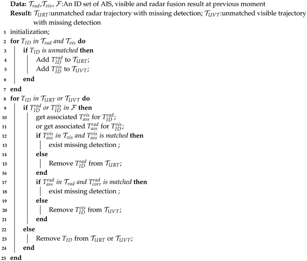
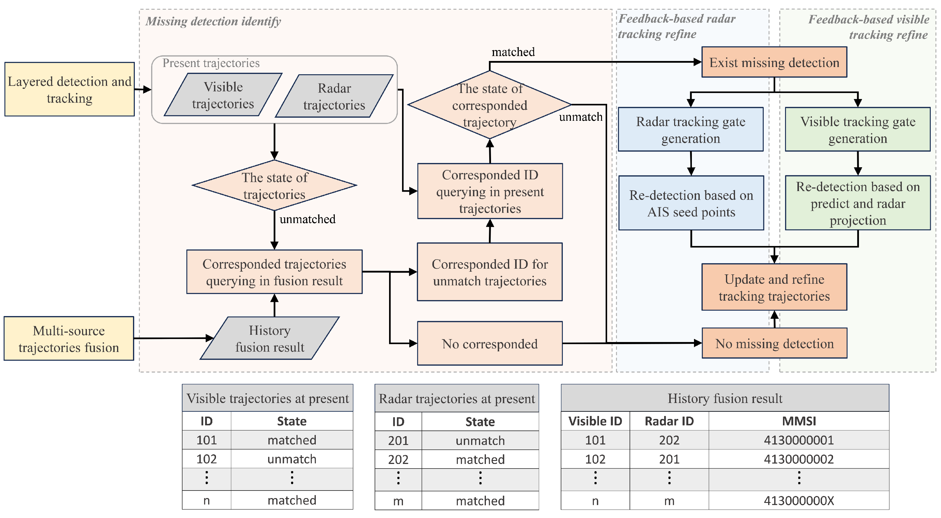
Figure 2.
The flowchart of the multi-stage detection and tracking method. The history fusion result feedback from the multi-source trajectories fusion module contains the MMSI, radar ID, and visible ID of the successfully fused target. By querying the fusion data of the previous and the layered detection and tracking results at present, it is determined whether single-modality data have missing detection. Re-detection and tracking with the help of multi-sources complementary data will update the missing trajectories.
Figure 3.
A typical radar scene of re-detection. The AIS data will be used as seed points to help complete the re-detection of radar echoes inside the tracking gate, avoiding clutter interference.
Figure 3.
A typical radar scene of re-detection. The AIS data will be used as seed points to help complete the re-detection of radar echoes inside the tracking gate, avoiding clutter interference.
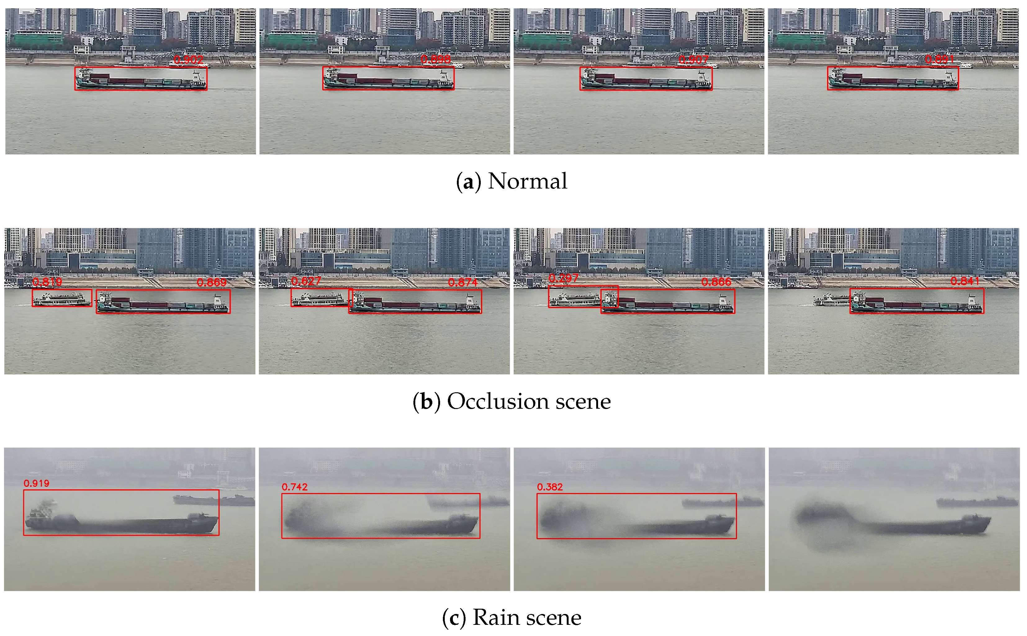
Figure 4.
Reduced confidence and missing detection caused by environmental interference. In a normal scene, detection boxes are stable and reliable, but environmental interference causes the target to be unable to recognize and the appearance features change dramatically, which will affect the tracking results.
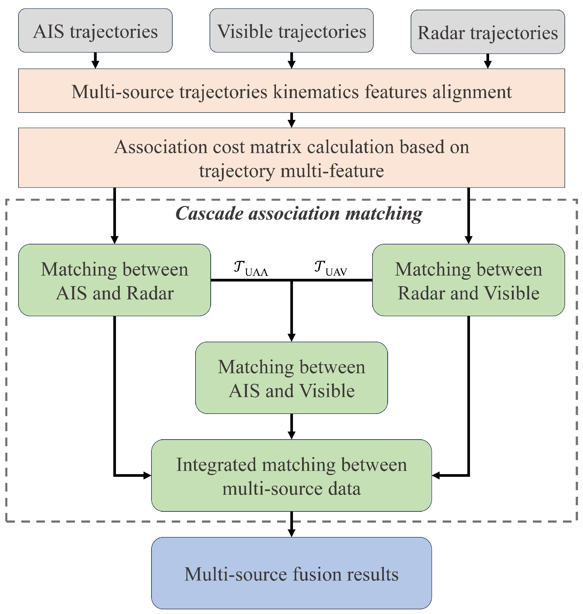
Figure 5.
The flowchart of multi-source trajectory fusion. We use the kinematics feature to measure trajectory similarity between multi-source data. And a cascade association matching method is specially designed to reduce the number of trajectories that need to be associated in a lower-precision coordinate system by associating the high-precision aligned data first.
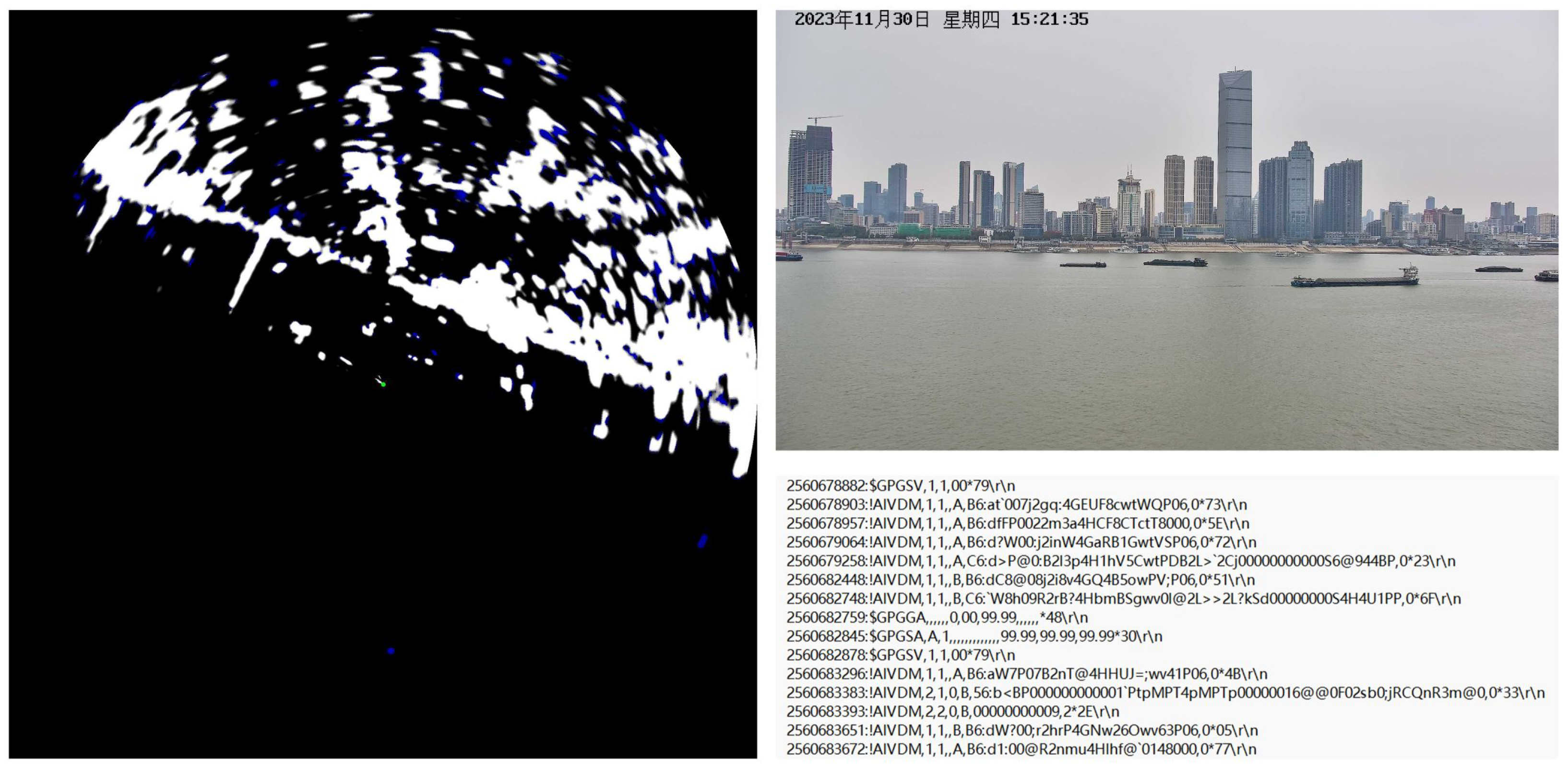
Figure 6.
Examples of collected data in WHUT-MSFVessel dataset, including radar images, visible images, and AIS coded messages.
Figure 6.
Examples of collected data in WHUT-MSFVessel dataset, including radar images, visible images, and AIS coded messages.
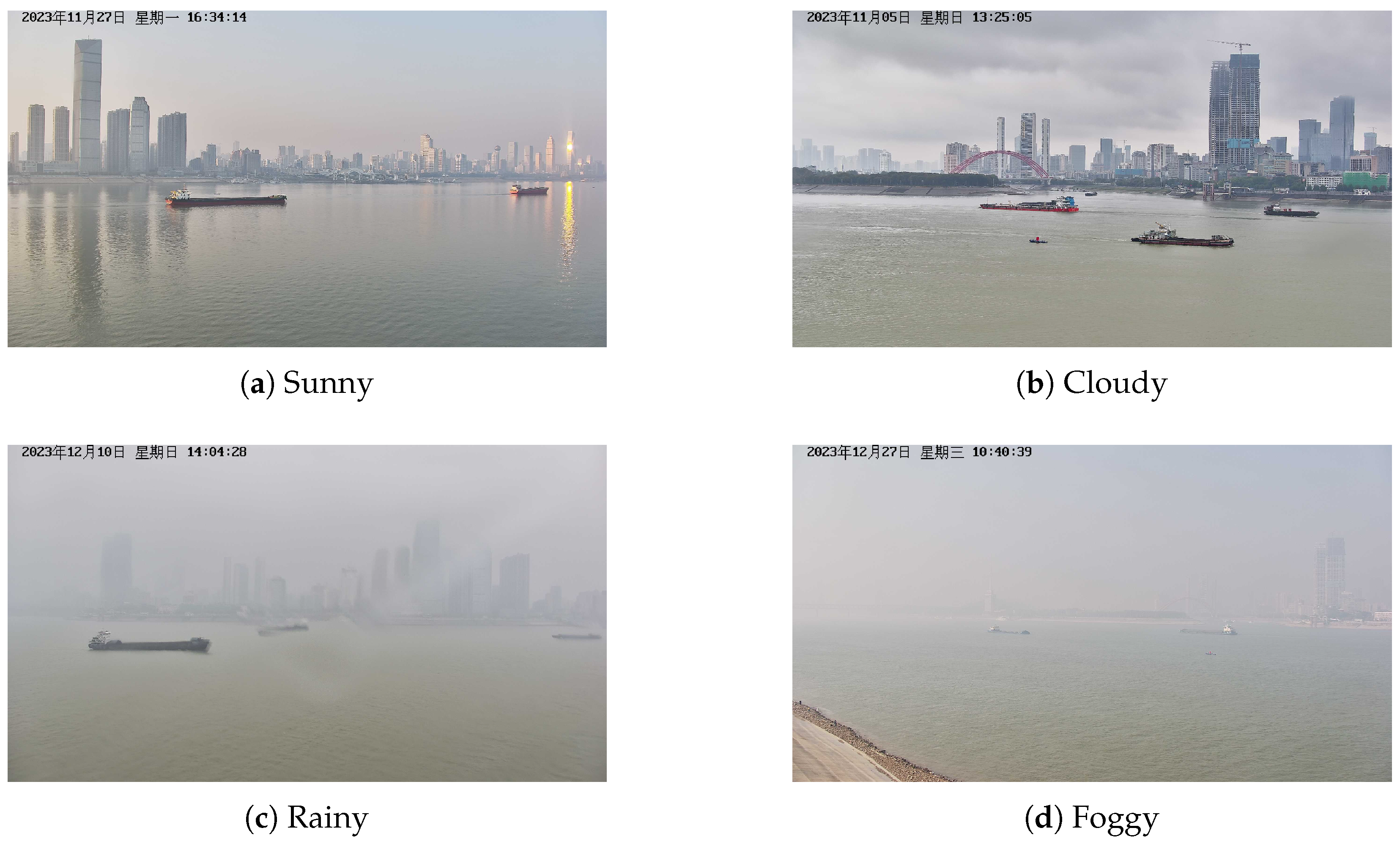
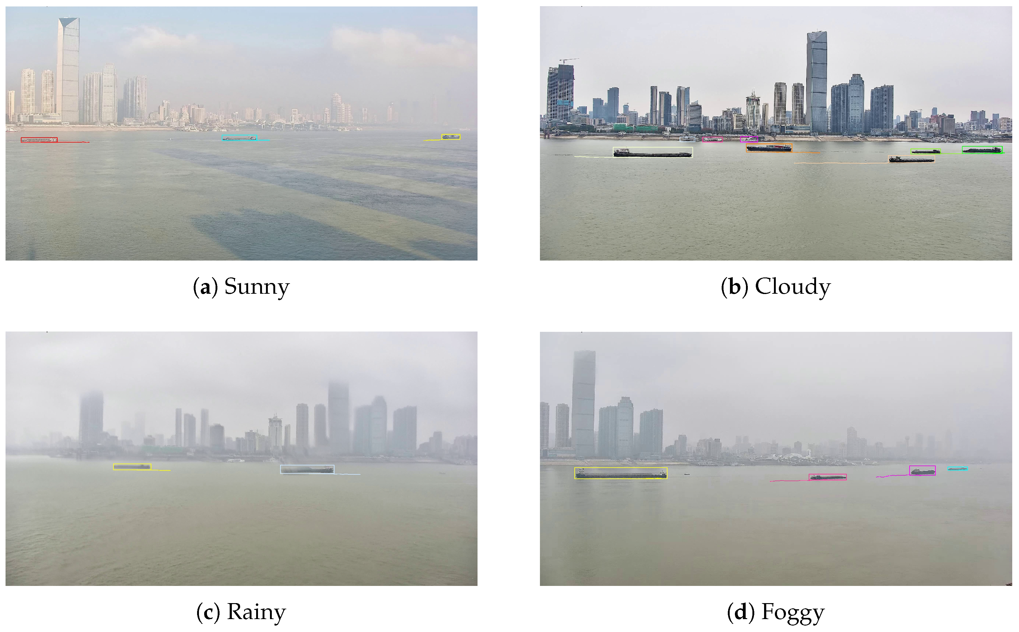
Figure 7.
Some samples of visible image representing different weather conditions in WHUT-MSFVessel dataset, including sunny, cloudy, rainy, and foggy.
Figure 7.
Some samples of visible image representing different weather conditions in WHUT-MSFVessel dataset, including sunny, cloudy, rainy, and foggy.
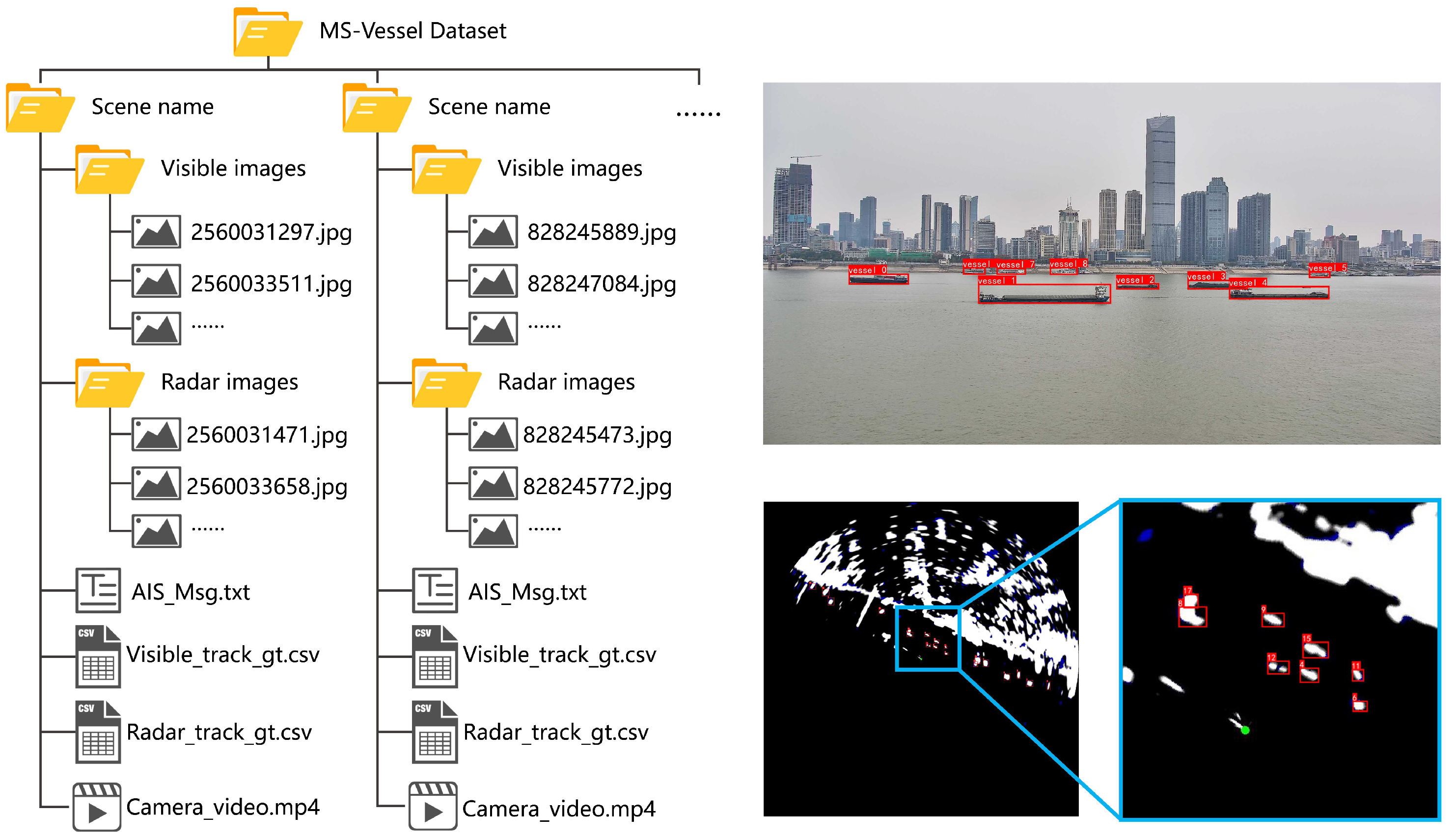
Figure 8.
The dataset structure and annotation examples. The data of each scene include AIS text file, synchronized visible and radar images, annotation data stored in csv files, and camera video. During the annotation process, bounding boxes are used to cover vessel targets, and each target is assigned a globally unique tracking ID.
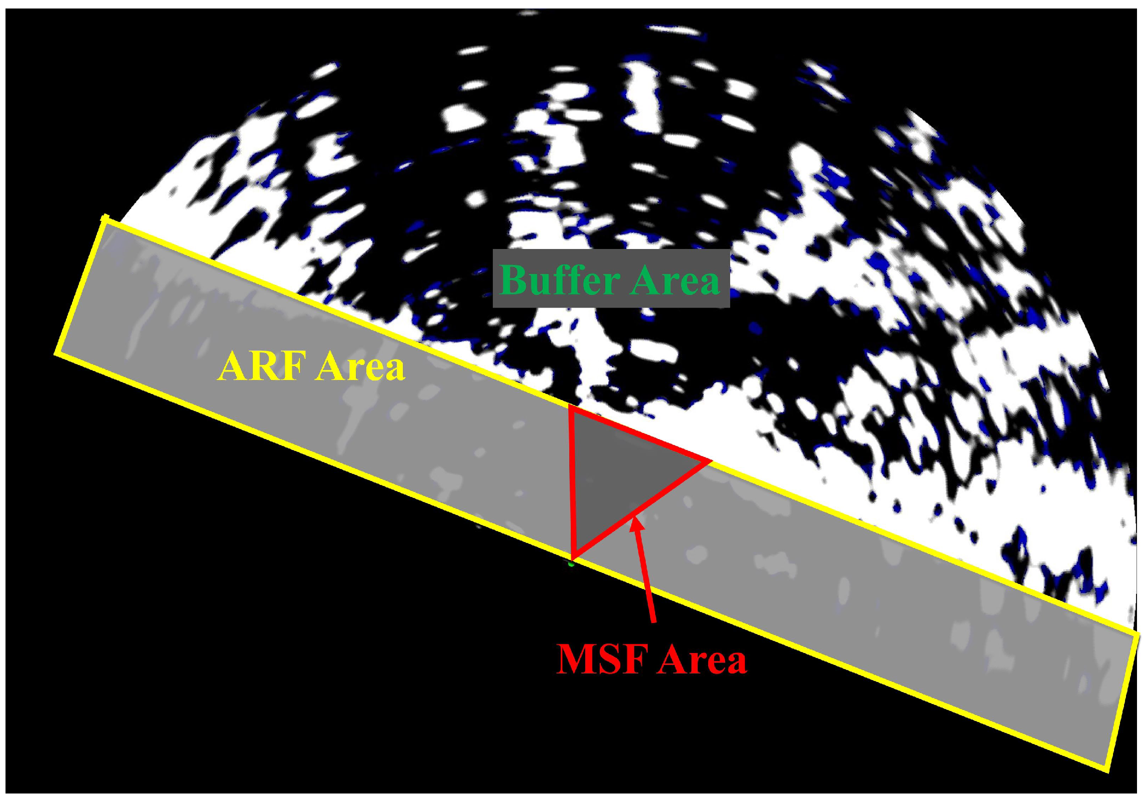
Figure 9.
Different areas in the multi-source perception scene. AIS data in the buffer area are cached before entering the fusion areas. In the ARF area, the AIS and radar trajectories are fused. The MSF area is the camera’s field of view; only this area contains AIS, radar, and visible data at the same time, so the multi-source fusion is carried out in this area.
Figure 10.
Radar tracking result compared with different methods. Errors in the tracking are marked by the red dotted circle. From top to bottom, the methods shown are (a) SORT, (b) Bytetrack, (c) BotSORT, and (d) our MSTrack.
Figure 10.
Radar tracking result compared with different methods. Errors in the tracking are marked by the red dotted circle. From top to bottom, the methods shown are (a) SORT, (b) Bytetrack, (c) BotSORT, and (d) our MSTrack.
Figure 11.
Some samples of radar tracking in different scenarios, including swerve, dense, and cross.
Figure 11.
Some samples of radar tracking in different scenarios, including swerve, dense, and cross.
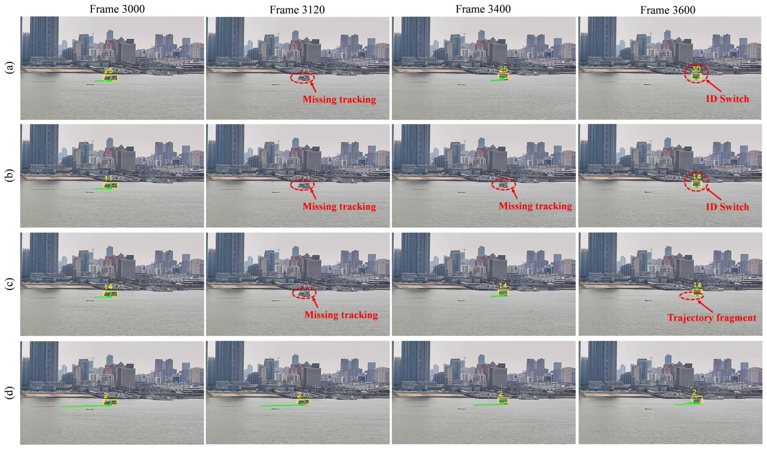
Figure 12.
Visible tracking result compared with different methods. Errors in the tracking are marked by the red dotted circle. From top to bottom, the methods shown are (a) DeepSORT, (b) Bytetrack, (c) BotSORT, and (d) our MSTrack.
Figure 12.
Visible tracking result compared with different methods. Errors in the tracking are marked by the red dotted circle. From top to bottom, the methods shown are (a) DeepSORT, (b) Bytetrack, (c) BotSORT, and (d) our MSTrack.
Figure 13.
Some samples of visible tracking in different weather conditions, including sunny, cloudy, rainy, and foggy.
Figure 13.
Some samples of visible tracking in different weather conditions, including sunny, cloudy, rainy, and foggy.
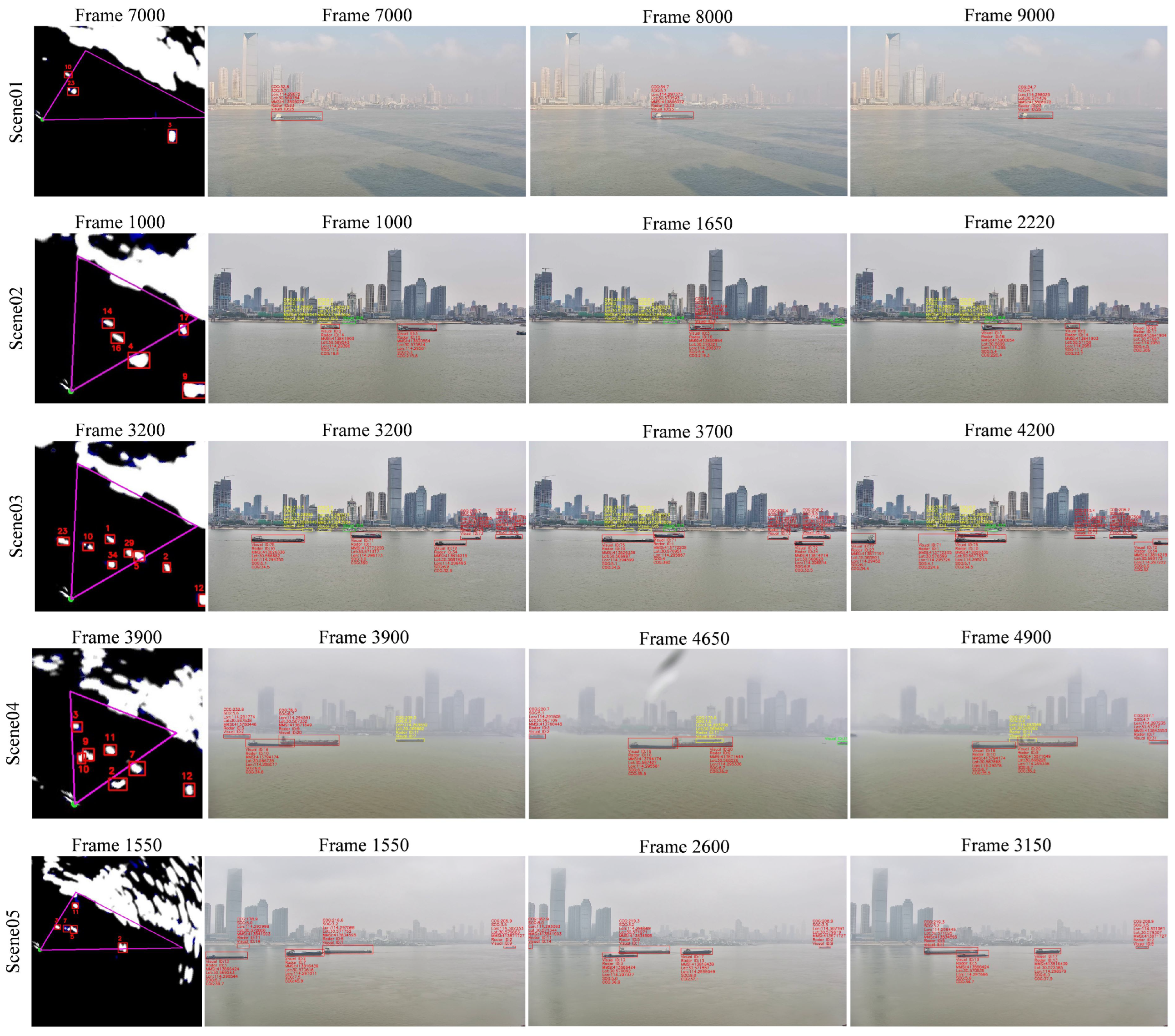
Figure 14.
The fusion result in the main view of visible images in different scenes.
Figure 14.
The fusion result in the main view of visible images in different scenes.
Table 1.
Most cited public accessible datasets for water surface perception compared with our WHUT-MSFVessel dataset.
Table 1.
Most cited public accessible datasets for water surface perception compared with our WHUT-MSFVessel dataset.
| Datasets | AIS | Radar | Visible |
|---|
| Piraeus AIS [47] | ✓ | | |
| OpenSARShip [48] | | ✓ | |
| HRSID [49] | | ✓ | |
| Seaship [50] | | | ✓ |
| MaSTr1325 [51] | | | ✓ |
| MaSTr1478 [52] | | | ✓ |
| FloW [53] | | ✓ | ✓ |
| FVessel [46] | ✓ | | ✓ |
| WHUT-MSFVessel (ours) | ✓ | ✓ | ✓ |
Table 2.
Detail of the WHUT-MSFVessel dataset. The “NR”, “NV”, “MN”, and “OC” represent the total number of radar targets, the total number of visible targets, the maximum number of targets in camera view, and the number of occluded targets, respectively.
Table 2.
Detail of the WHUT-MSFVessel dataset. The “NR”, “NV”, “MN”, and “OC” represent the total number of radar targets, the total number of visible targets, the maximum number of targets in camera view, and the number of occluded targets, respectively.
| Scene | Duration | NR | NV | MN | OC | Weather |
|---|
| scene01 | 09m06s | 12 | 4 | 3 | 1 | Sunny |
| scene02 | 04m20s | 25 | 7 | 6 | 3 | Cloudy |
| scene03 | 08m20s | 21 | 10 | 9 | 1 | Cloudy |
| scene04 | 07m01s | 17 | 6 | 5 | 4 | Rainy |
| scene05 | 07m16s | 15 | 6 | 5 | 2 | Foggy |
| scene06 | 15m20s | 32 | 10 | 6 | 4 | Sunny |
| scene07 | 11m50s | 11 | 5 | 3 | 0 | Sunny |
| scene08 | 14m54s | 30 | 11 | 6 | 4 | Sunny |
| scene09 | 18m38s | 17 | 10 | 5 | 3 | Sunny |
| scene10 | 10m07s | 19 | 8 | 4 | 2 | Cloudy |
| scene11 | 21m22s | 12 | 8 | 6 | 0 | Cloudy |
| scene12 | 13m21s | 20 | 12 | 6 | 4 | Cloudy |
| scene13 | 18m16s | 18 | 7 | 3 | 0 | Rainy |
| scene14 | 14m48s | 21 | 5 | 4 | 1 | Rainy |
| scene15 | 21m23s | 25 | 6 | 4 | 2 | Rainy |
| scene16 | 17m02s | 18 | 7 | 3 | 2 | Rainy |
| scene17 | 23m12s | 33 | 9 | 6 | 3 | Rainy |
| scene18 | 30m17s | 19 | 6 | 2 | 2 | Foggy |
| scene19 | 21m45s | 15 | 5 | 3 | 0 | Foggy |
| scene20 | 19m24s | 20 | 9 | 5 | 2 | Foggy |
| scene21 | 31m36s | 27 | 9 | 6 | 0 | Foggy |
| scene22 | 41m07s | 31 | 12 | 5 | 4 | Foggy |
Table 3.
Quantitative evaluation results of various radar tracking methods for comparison in different scenes. The comparative tracking methods include SORT [
37], Bytetrack [
39], and BotSORT [
58].
Table 3.
Quantitative evaluation results of various radar tracking methods for comparison in different scenes. The comparative tracking methods include SORT [
37], Bytetrack [
39], and BotSORT [
58].
| Scene | Method | MOTA↑ | IDP↑ | IDR↑ | IDF1↑ | IDSw↓ | MT↑ | ML↓ |
|---|
| scece01 | SORT | 0.601 | 0.726 | 0.573 | 0.640 | 15 | 7 | 2 |
| Bytetrack | 0.688 | 0.734 | 0.572 | 0.643 | 14 | 8 | 1 |
| BotSORT | 0.691 | 0.736 | 0.574 | 0.645 | 14 | 8 | 1 |
| MSTrack | 0.830 | 0.776 | 0.724 | 0.749 | 7 | 10 | 0 |
| scece02 | SORT | 0.795 | 0.864 | 0.717 | 0.784 | 14 | 16 | 2 |
| Bytetrack | 0.802 | 0.866 | 0.743 | 0.801 | 12 | 18 | 2 |
| BotSORT | 0.802 | 0.897 | 0.769 | 0.828 | 11 | 18 | 2 |
| MSTrack | 0.912 | 0.891 | 0.886 | 0.888 | 5 | 23 | 1 |
| scene03 | SORT | 0.739 | 0.683 | 0.521 | 0.591 | 51 | 12 | 1 |
| Bytetrack | 0.758 | 0.792 | 0.631 | 0.703 | 24 | 14 | 1 |
| BotSORT | 0.762 | 0.796 | 0.634 | 0.706 | 23 | 14 | 1 |
| MSTrack | 0.896 | 0.798 | 0.739 | 0.767 | 23 | 19 | 0 |
| scene04 | SORT | 0.716 | 0.655 | 0.508 | 0.572 | 30 | 12 | 2 |
| Bytetrack | 0.701 | 0.712 | 0.530 | 0.607 | 23 | 13 | 2 |
| BotSORT | 0.700 | 0.711 | 0.529 | 0.607 | 21 | 13 | 1 |
| MSTrack | 0.869 | 0.855 | 0.807 | 0.830 | 11 | 17 | 0 |
| scene05 | SORT | 0.727 | 0.728 | 0.568 | 0.638 | 12 | 10 | 2 |
| Bytetrack | 0.703 | 0.807 | 0.588 | 0.680 | 13 | 10 | 2 |
| BotSORT | 0.732 | 0.812 | 0.597 | 0.688 | 12 | 10 | 2 |
| MSTrack | 0.875 | 0.869 | 0.879 | 0.874 | 6 | 14 | 0 |
| Average | SORT | 0.704 | 0.719 | 0.565 | 0.632 | 122 | 57 | 9 |
| Bytetrack | 0.723 | 0.774 | 0.601 | 0.676 | 86 | 63 | 8 |
| BotSORT | 0.729 | 0.779 | 0.607 | 0.682 | 81 | 63 | 7 |
| MSTrack | 0.872 | 0.828 | 0.794 | 0.811 | 52 | 83 | 1 |
Table 4.
Quantitative evaluation results of various visible tracking methods for comparison in different scenes. The comparative tracking methods include DeepSORT [
38], Bytetrack [
39], and BotSORT [
58].
Table 4.
Quantitative evaluation results of various visible tracking methods for comparison in different scenes. The comparative tracking methods include DeepSORT [
38], Bytetrack [
39], and BotSORT [
58].
| Scene | Method | MOTA↑ | IDP↑ | IDR↑ | IDF1↑ | IDSw↓ | MT↑ | ML↓ |
|---|
| scece01 | DeepSORT | 0.846 | 0.855 | 0.742 | 0.795 | 10 | 3 | 0 |
| Bytetrack | 0.844 | 0.982 | 0.838 | 0.904 | 6 | 4 | 0 |
| BotSORT | 0.885 | 0.987 | 0.855 | 0.917 | 4 | 4 | 0 |
| MSTrack | 0.941 | 0.979 | 0.907 | 0.942 | 3 | 4 | 0 |
| scece02 | DeepSORT | 0.906 | 0.868 | 0.810 | 0.838 | 14 | 5 | 1 |
| Bytetrack | 0.906 | 0.875 | 0.813 | 0.843 | 12 | 5 | 0 |
| BotSORT | 0.908 | 0.890 | 0.827 | 0.858 | 7 | 5 | 0 |
| MSTrack | 0.935 | 0.964 | 0.947 | 0.956 | 5 | 6 | 0 |
| scene03 | DeepSORT | 0.935 | 0.947 | 0.945 | 0.946 | 13 | 9 | 1 |
| Bytetrack | 0.98 | 0.962 | 0.959 | 0.961 | 6 | 9 | 1 |
| BotSORT | 0.979 | 0.963 | 0.960 | 0.961 | 4 | 9 | 1 |
| MSTrack | 0.981 | 0.986 | 0.994 | 0.990 | 1 | 10 | 0 |
| scene04 | DeepSORT | 0.848 | 0.619 | 0.569 | 0.593 | 28 | 5 | 0 |
| Bytetrack | 0.858 | 0.762 | 0.696 | 0.728 | 17 | 5 | 0 |
| BotSORT | 0.870 | 0.778 | 0.710 | 0.742 | 14 | 6 | 0 |
| MSTrack | 0.914 | 0.895 | 0.882 | 0.889 | 4 | 6 | 0 |
| scene05 | DeepSORT | 0.833 | 0.678 | 0.593 | 0.633 | 17 | 3 | 2 |
| Bytetrack | 0.835 | 0.846 | 0.738 | 0.788 | 9 | 4 | 1 |
| BotSORT | 0.836 | 0.792 | 0.691 | 0.738 | 9 | 4 | 1 |
| MSTrack | 0.911 | 0.889 | 0.871 | 0.880 | 2 | 5 | 0 |
| Average | DeepSORT | 0.882 | 0.796 | 0.733 | 0.763 | 82 | 25 | 4 |
| Bytetrack | 0.884 | 0.894 | 0.814 | 0.852 | 50 | 27 | 2 |
| BotSORT | 0.897 | 0.889 | 0.815 | 0.850 | 38 | 28 | 2 |
| MSTrack | 0.938 | 0.939 | 0.920 | 0.929 | 15 | 31 | 0 |
Table 5.
Quantitative evaluation results of multi-source heterogeneous data fusion in different scenes.
Table 5.
Quantitative evaluation results of multi-source heterogeneous data fusion in different scenes.
| Scene | TPF | PPF | FPF | FNF | Accuracy |
|---|
| scene01 | 263 | 0 | 4 | 12 | 0.943 |
| scene02 | 559 | 6 | 2 | 49 | 0.917 |
| scene03 | 1254 | 27 | 15 | 89 | 0.904 |
| scene04 | 807 | 5 | 5 | 60 | 0.920 |
| scene05 | 598 | 9 | 6 | 69 | 0.883 |
Table 6.
Processing time of different modules in multiple scenes, including detection, tracking, fusion and overall process (unit: ms).
Table 6.
Processing time of different modules in multiple scenes, including detection, tracking, fusion and overall process (unit: ms).
| Scene | Trajectory Num | Detection | Tracking | Fusion | Overall |
|---|
| scene01 | 16 | 16.6 | 2.8 | 2.4 | 24.5 |
| scene02 | 32 | 17.1 | 5.6 | 5.3 | 33.2 |
| scene03 | 31 | 17.2 | 5.8 | 5.9 | 34.8 |
| scene04 | 23 | 16.8 | 4.2 | 4.7 | 31.7 |
| scene05 | 21 | 16.7 | 4.0 | 4.5 | 31.2 |
| Average | - | 16.9 | 4.5 | 4.6 | 31.1 |

 ,
, 


