

Quantifying and Forecasting Emission Reductions in Urban Mobility: An IoT-Driven Bike-Sharing Analysis


Abstract
1. Introduction
- RQ1: What is the state-of-the-art of machine learning models for estimating GHG emissions in large cities?
- RQ2: How can IoT sensors and predictive machine learning models be used to accurately quantify the environmental impact of the bike-sharing system in Madrid, specifically in terms of CO2 and NOx emission reductions?
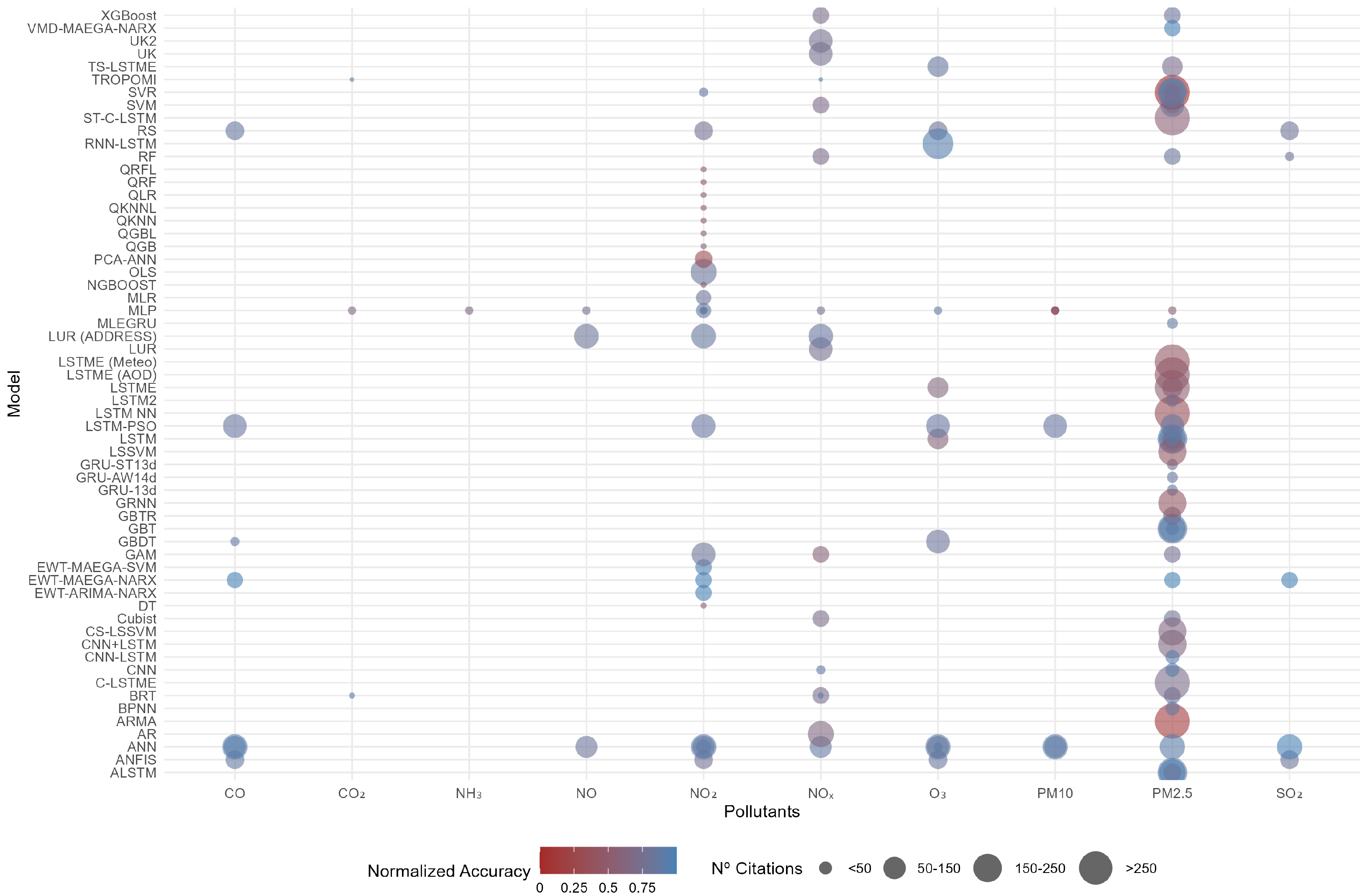
2. Machine Learning Models for Urban GHG Prediction
Comparative Analysis of Predictive Models for Urban Air Pollution
3. Methods
3.1. Data
3.2. Materials
3.3. Procedure
3.4. Analysis
4. Results
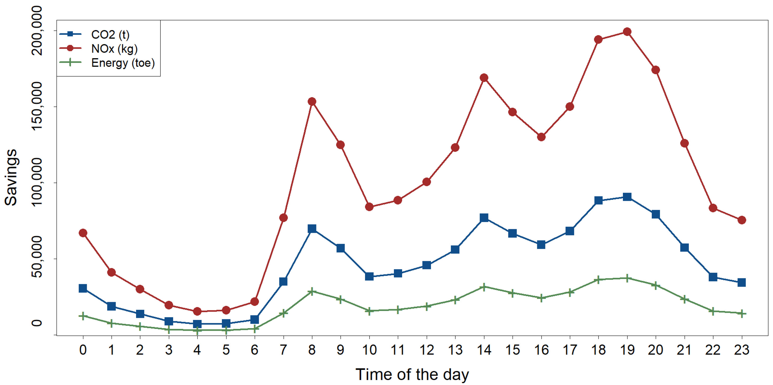
4.1. Quantifying Greenhouse Gas Emission Savings
4.2. Anticipating Greenhouse Gas Emission Savings
5. Discussion and Conclusions
Author Contributions
Funding
Institutional Review Board Statement
Informed Consent Statement
Data Availability Statement
Conflicts of Interest
Appendix A. Machine Learning Models Anticipating Pollutants in Urban Areas

| Reference | Model | Pollutants | Accuracy /RMSE |
|---|---|---|---|
| Zhang et al. [24] | TROPOMI | 0.97 / — | |
| TROPOMI | 0.97 / — | ||
| Li et al. [26] | SVM | PM2.5 | 0.75 / — |
| GAM | 0.76 / — | ||
| RF | 0.83 / — | ||
| BRT | 0.83 / — | ||
| XGBoost | 0.82 / — | ||
| Cubist | 0.81 / — | ||
| SVM | 0.69 / — | ||
| GAM | 0.59 / — | ||
| RF | 0.71 / — | ||
| BRT | 0.71 / — | ||
| XGBoost | 0.70 / — | ||
| Cubist | 0.70 / — | ||
| Wen et al. [27] | BRT | 0.93 / — | |
| BRT | 0.9 / — | ||
| Zeinalnezhad et al. [28] | ANFIS | CO | 0.8693 / — |
| RS | CO | 0.8445 / — | |
| ANFIS | 0.8011 / — | ||
| RS | 0.8001 / — | ||
| ANFIS | O3 | 0.8350 / — | |
| RS | O3 | 0.7830 / — | |
| ANFIS | NO2 | 0.7640 / — | |
| RS | NO2 | 0.7602 / — | |
| Arhami et al. [29] | ANN | CO | 0.92 / — |
| ANN | O3 | 0.77 / — | |
| ANN | 0.87 / — | ||
| ANN | 0.87 / — | ||
| ANN | 0.85 / — | ||
| ANN | NO | 0.82 / — | |
| Goulier et al. [30] | MLP | 0.685 / — | |
| MLP | 0.648 / — | ||
| MLP | NO | 0.751 / — | |
| MLP | 0.915 / — | ||
| MLP | 0.751 / — | ||
| MLP | O3 | 0.871 / — | |
| MLP | 0.315 / — | ||
| MLP | 0.587 / — | ||
| MLP | 0.536 / — | ||
| MLP | 0.449 / — | ||
| Shi and Harrison [31] | OLS | 0.83 / — | |
| AR | 0.65 / — | ||
| Vasseur and Aznarte [32] | QRF | — / 22.62 | |
| QRFL | — / 19.12 | ||
| QKNN | — / 20.73 | ||
| QKNNL | — / 18.4 | ||
| QGB | — / 16.09 | ||
| QGBL | — / 16.14 | ||
| QLR | — / 19.44 | ||
| MLP | — / 18.16 | ||
| NGBOOST | — / 18.52 | ||
| DT | — / 18.69 | ||
| Liu et al. [33] | EWT-MAEGA-NARX | — / 0.1793 | |
| EWT-MAEGA-NARX | — / 0.0347 | ||
| EWT-MAEGA-NARX | — / 0.0969 | ||
| EWT-MAEGA-NARX | CO | — / 0.0041 | |
| VMD-MAEGA-NARX | — / 0.3361 | ||
| EWT-MAEGA-SVM | — / 0.9451 | ||
| EWT-ARIMA-NARX | — / 0.3548 | ||
| Mercer et al. [47] | UK | 0.75 / — | |
| LUR | 0.74 / — | ||
| UK2 | 0.75 / — | ||
| Su et al. [46] | LUR (ADDRESS) | NO | 0.81 / — |
| LUR (ADDRESS) | 0.86 / — | ||
| LUR (ADDRESS) | 0.85 / — | ||
| Wen et al. [36] | C-LSTME | — / 12.08 | |
| ST-C-LSTM | — / 17.76 | ||
| LSTME | — / 18.25 | ||
| LSTME (AOD) | — / 21.17 | ||
| LSTME (Meteo) | — / 22.22 | ||
| LSTM NN | — / 25.95 | ||
| ARMA | — / 34.40 | ||
| SVR | — / 39.92 | ||
| Mao et al. [34] | TS-LSTME | 0.72 / — | |
| TS-LSTME | O3 | 0.86 / — | |
| LSTME | 0.52 / — | ||
| LSTME | O3 | 0.63 / — | |
| LSTM | 0.52 / — | ||
| LSTM | O3 | 0.60 / — | |
| Chang et al. [37] | GBT | 0.83 / — | |
| SVR | 0.73 / — | ||
| LSTM | 0.71 / — | ||
| LSTM2 | 0.73 / — | ||
| Chang et al. [38] | GBT | 0.86 / — | |
| SVR | 0.87 / — | ||
| LSTM | 0.85 / — | ||
| ALSTM | 0.88 / — | ||
| Rybarczyk and Zalakeviciute [64] | GBT | — / 1.59 | |
| SVR | — / 2.77 | ||
| LSTM | — / 1.59 | ||
| ALSTM | — / 0.44 | ||
| Masih [39] | LSTM | 0.78 / — | |
| SVR | 0.73 / — | ||
| GBTR | 0.76 / — | ||
| ALSTM | 0.82 / — | ||
| Mokhtari et al. [40] | LSTM | 0.91 / — | |
| SVR | 0.85 / — | ||
| ANN | O3 | 0.89 / — | |
| RF | 0.82 / — | ||
| GBDT | CO | 0.87 / — | |
| CNN | 0.88 / — | ||
| Lin et al. [41] | GRU-13d | 0.91 / — | |
| GRU-AW14d | 0.85 / — | ||
| GRU-ST13d | 0.78 / — | ||
| MLEGRU | 0.88 / — | ||
| Al-Janabi et al. [65] | LSTM-PSO | 0.85 / — | |
| LSTM-PSO | 0.85 / — | ||
| LSTM-PSO | 0.85 / — | ||
| LSTM-PSO | CO | 0.85 / — | |
| LSTM-PSO | O3 | 0.85 / — | |
| SVM | 0.78 / — | ||
| GAM | 0.81 / — | ||
| GBDT | O3 | 0.82 / — | |
| Mishra and Goyal [66] | PCA-ANN | 0.318 / — | |
| Freeman et al. [67] | RNN-LSTM | O3 | — / 2.5 |
| Qin et al. [68] | CNN+LSTM | — / 14.3 | |
| Sun and Sun [69] | CS-LSSVM | — / 14.47 | |
| LSSVM | — / 21.75 | ||
| GRNN | — / 22.89 | ||
| Yang et al. [43] | CNN | 0.931 / — | |
| LSTM | 0.92 / — | ||
| CNN-LSTM | 0.92 / — | ||
| BPNN | 0.875 / — | ||
| Maleki et al. [44] | ANN | O3 | 0.90 / — |
| ANN | 0.91 / — | ||
| ANN | 0.99 / — | ||
| ANN | 0.91 / — | ||
| ANN | 0.91 / — | ||
| ANN | CO | 0.94 / — | |
| Shams et al. [45] | ANN | 0.89 / — | |
| MLR | 0.81 / — | ||
| MLP | 0.89 / — |
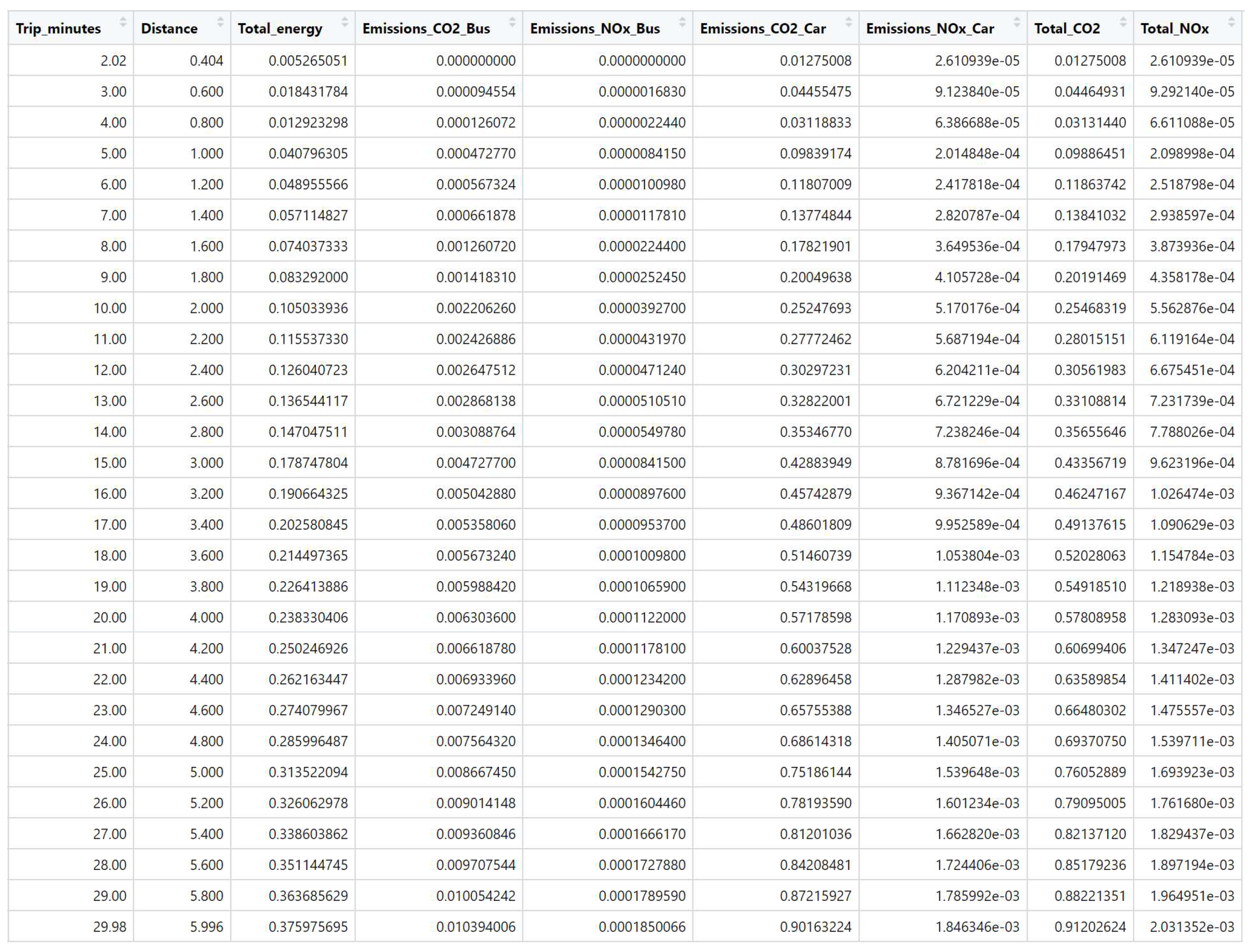
Appendix B. Equivalent Energy Savings
Appendix C. Structure of the Working Dataset
| CHARACTER | ||||
|---|---|---|---|---|
| skim_variable | n_missing | complete_rate | min | max |
| geolocation_unlock | 0 | 1.0 | 53 | 75 |
| address_unlock | 0 | 1.0 | 15 | 68 |
| geolocation_lock | 0 | 1.0 | 53 | 75 |
| address_lock | 0 | 1.0 | 15 | 68 |
| unlock_station_name | 0 | 1.0 | 10 | 58 |
| lock_station_name | 0 | 1.0 | 10 | 58 |
| day | 0 | 1.0 | 2 | 2 |
| hour | 0 | 1.0 | 2 | 2 |
| daysweek | 0 | 1.0 | 5 | 9 |
| DATE | ||||
| skim_variable | n_missing | complete_rate | min | max |
| date | 0 | 1.0 | 2023-01-01 | 2023-01-31 |
| FACTOR | ||||
| skim_variable | n_missing | complete_rate | ordered | n_unique |
| station_unlock | 0 | 1.0 | FALSE | 260 |
| dock_unlock | 0 | 1.0 | FALSE | 30 |
| station_lock | 0 | 1.0 | FALSE | 260 |
| dock_lock | 0 | 1.0 | FALSE | 30 |
| NUMERIC | ||||
| skim_variable | n_missing | complete_rate | mean | sd |
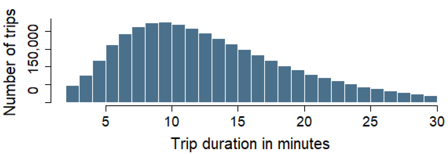
| trip_minutes | 0 | 1.0 | 12.20849 | 5.980459 |
| POSIXCT | ||||
| skim_variable | n_missing | complete_rate | min | max |
| unlock_date | 0 | 1.0 | 2022-01-01 00:01:45 | 2022-12-31 23:59:44 |
| lock_date | 0 | 1.0 | 2022-01-01 00:10:05 | 2022-12-31 19:02:43 |
Appendix D. Extended Analysis of BSS in Madrid
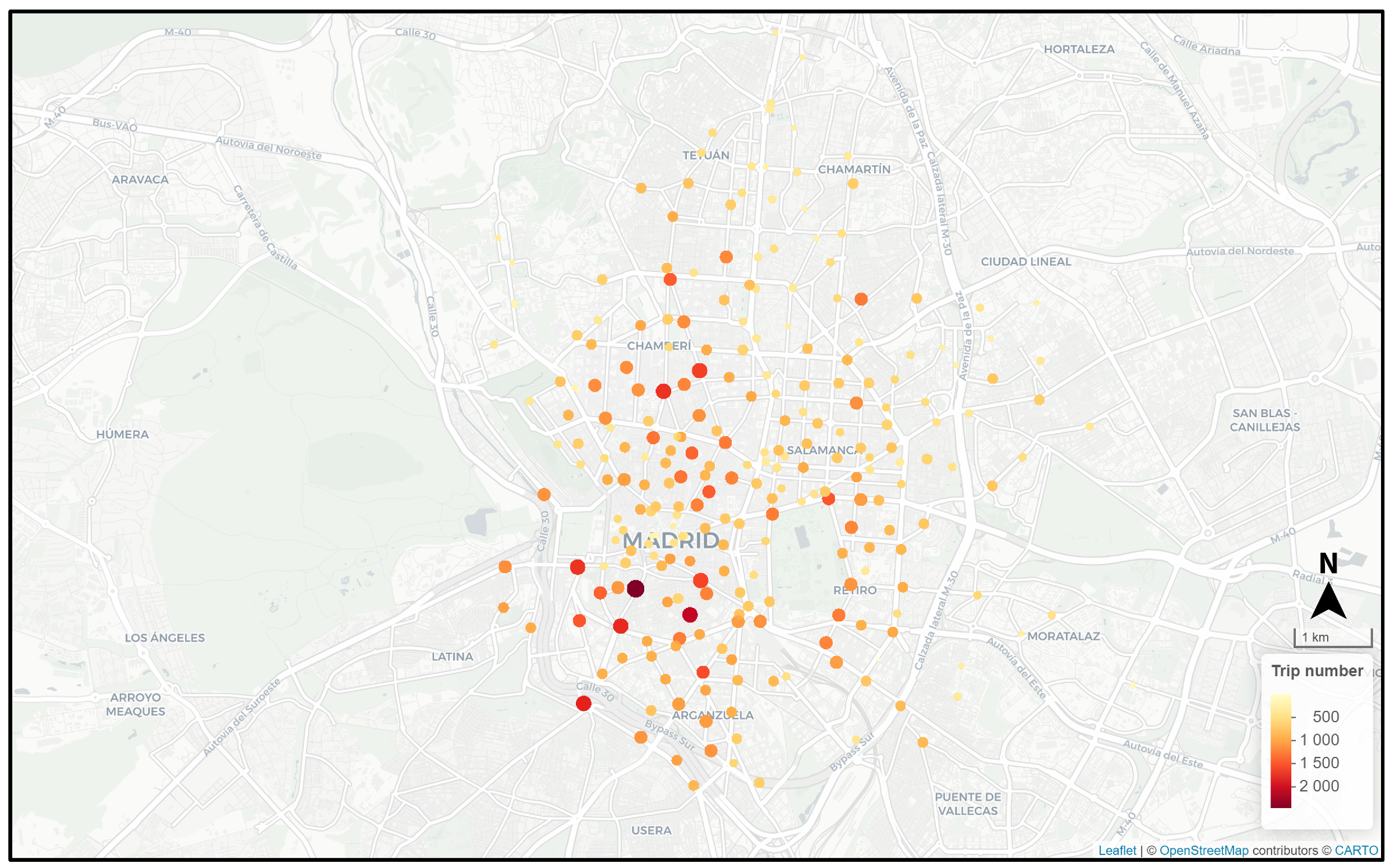
Appendix D.1. Docking Station Usage Distribution
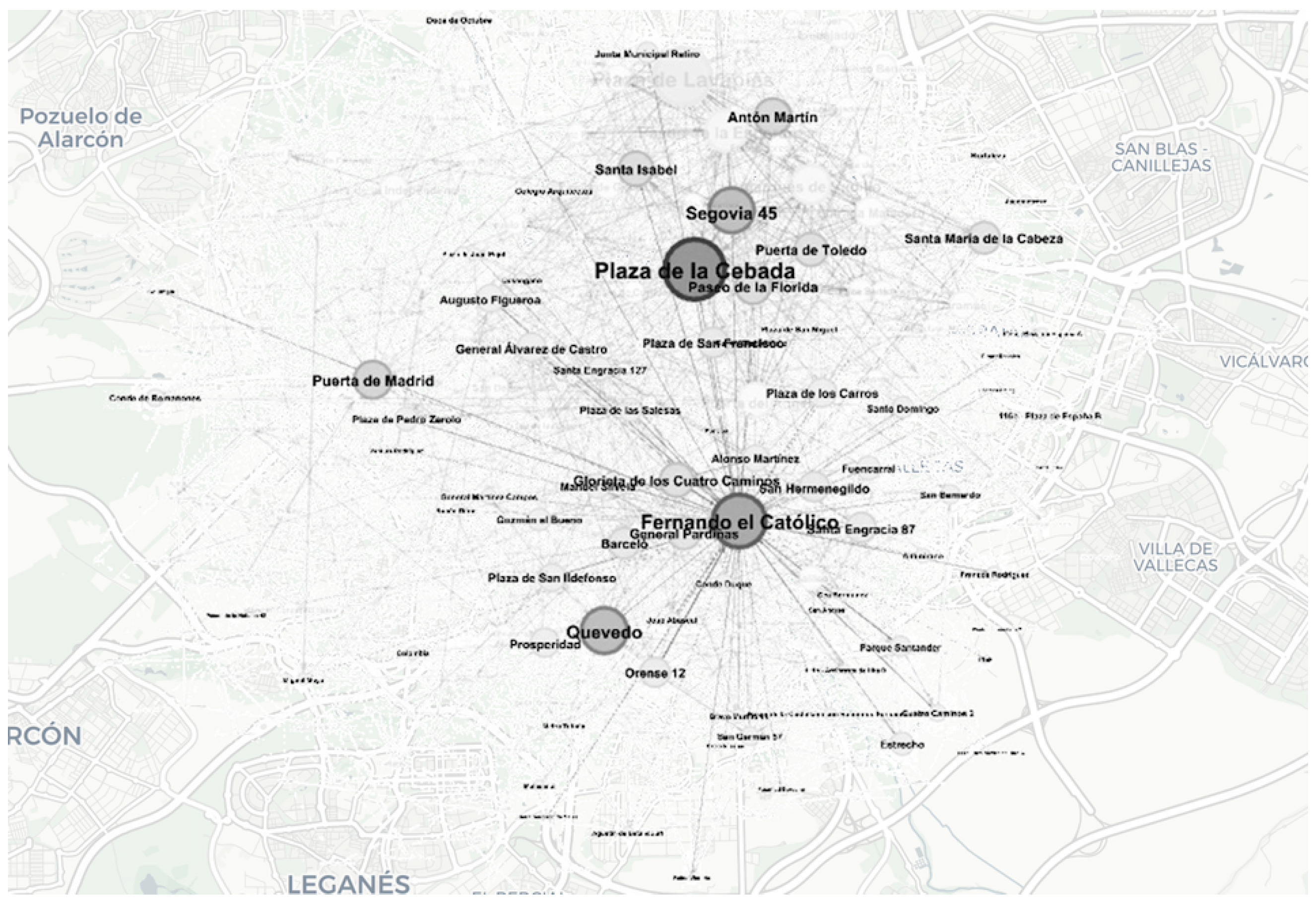
Appendix D.2. Connectivity of Docking Stations
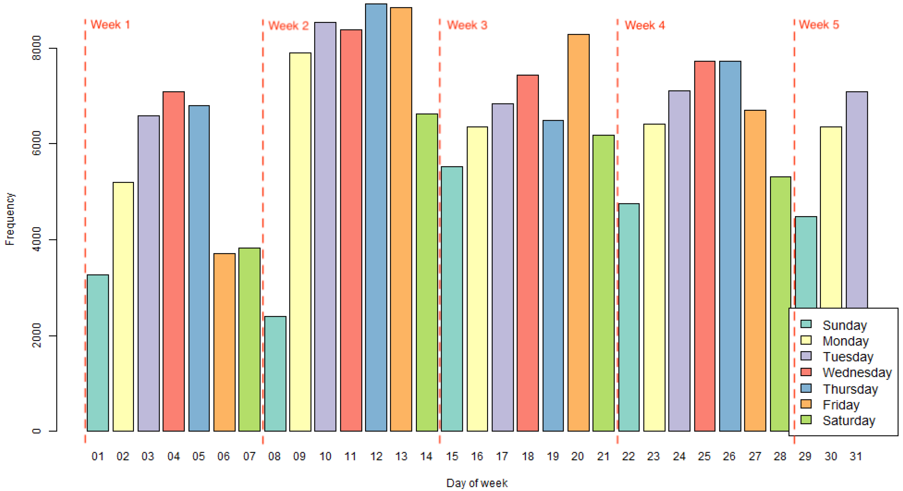
Appendix D.3. Weekly and Monthly Usage Patterns
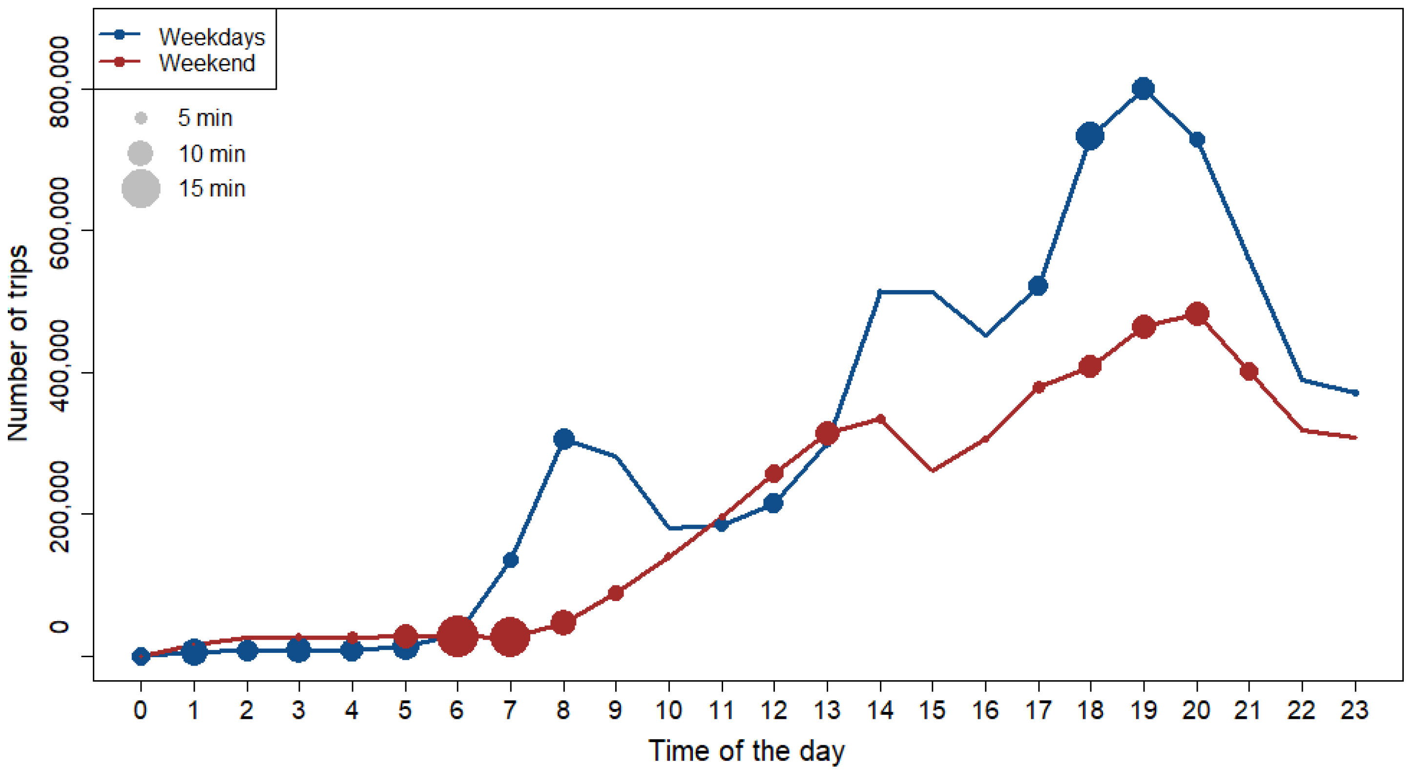
Appendix D.4. Daily Usage Patterns

Appendix D.5. Leisure and Working Days
References
- GrowLondon. Smart Mobility—Grow London. 2024. Available online: https://www.grow.london/set-up-in-london/sectors/urban/smart-mobility (accessed on 6 September 2024).
- AytoMadrid. Movilidad Sostenible—Madrid 360. 2024. Available online: https://www.madrid360.es/movilidad-sostenible/ (accessed on 6 September 2024).
- NYCityDept. New York City Mobility Report. 2024. Available online: https://www.nyc.gov/html/dot/html/about/mobilityreport.shtml (accessed on 6 September 2024).
- ParisRegion. Mobility & Transportation—Choose Paris Region. 2024. Available online: https://www.chooseparisregion.org/industries/Mobility-Transportation (accessed on 6 September 2024).
- Drosouli, I.; Voulodimos, A.; Mastorocostas, P.; Miaoulis, G.; Ghazanfarpour, D. A Spatial-Temporal Graph Convolutional Recurrent Network for Transportation Flow Estimation. Sensors 2023, 23, 7534. [Google Scholar] [CrossRef] [PubMed]
- Lee, J.S.; Chen, Z.H.; Hong, Y. Enhancing Urban Mobility with Self-Tuning Fuzzy Logic Controllers for Power-Assisted Bicycles in Smart Cities. Sensors 2024, 24, 1552. [Google Scholar] [CrossRef]
- Zguira, Y.; Rivano, H.; Meddeb, A. Internet of Bikes: A DTN Protocol with Data Aggregation for Urban Data Collection. Sensors 2018, 18, 2819. [Google Scholar] [CrossRef] [PubMed]
- Puyol, J.L.M.; Baeza, V.M. Bicycle sharing system using an iot network. In Proceedings of the 2021 Global Congress on Electrical Engineering (GC-ElecEng), Valencia, Spain, 10–12 December 2021; IEEE: Piscataway, NJ, USA, 2021; pp. 131–135. [Google Scholar]
- Kon, F.; Ferreira, É.C.; de Souza, H.A.; Duarte, F.; Santi, P.; Ratti, C. Abstracting mobility flows from bike-sharing systems. Public Transp. 2022, 14, 545–581. [Google Scholar]
- Gao, P.; Li, J. Understanding sustainable business model: A framework and a case study of the bike-sharing industry. J. Clean. Prod. 2020, 267, 122229. [Google Scholar]
- Karthika, K.; Nithya, A.; Sujatha, M.; Kovarasan, R.K.; Mahesh, A.; Murugan, S. Advancing Bike Sharing Security with SVM and IoT-Enabled Tracking and Anti-Theft Measures. In Proceedings of the 2024 2nd International Conference on Sustainable Computing and Smart Systems (ICSCSS), Coimbatore, India, 10–12 July 2024; IEEE: Piscataway, NJ, USA, 2024; pp. 351–356. [Google Scholar]
- Guo, D.; Yao, E.; Liu, S.; Chen, R.; Hong, J.; Zhang, J. Exploring the role of passengers’ attitude in the integration of dockless bike-sharing and public transit: A hybrid choice modeling approach. J. Clean. Prod. 2023, 384, 135627. [Google Scholar]
- Guo, Y.; He, S.Y. Built environment effects on the integration of dockless bike-sharing and the metro. Transp. Res. Part D Transp. Environ. 2020, 83, 102335. [Google Scholar]
- Zhang, H.; Zhuge, C.; Jia, J.; Shi, B.; Wang, W. Green travel mobility of dockless bike-sharing based on trip data in big cities: A spatial network analysis. J. Clean. Prod. 2021, 313, 127930. [Google Scholar]
- Wang, L.; Zhou, K.; Zhang, S.; Moudon, A.V.; Wang, J.; Zhu, Y.G.; Sun, W.; Lin, J.; Tian, C.; Liu, M. Designing bike-friendly cities: Interactive effects of built environment factors on bike-sharing. Transp. Res. Part D Transp. Environ. 2023, 117, 103670. [Google Scholar]
- Qiu, L.Y.; He, L. Bike Sharing and the Economy, the Environment, and Health-Related Externalities. Sustainability 2018, 10, 1145. [Google Scholar] [CrossRef]
- Guo, Y.; Yang, L.; Chen, Y. Bike Share Usage and the Built Environment: A Review. Front. Public Health 2022, 10, 848169. [Google Scholar] [CrossRef] [PubMed]
- Tao, J.; Zhou, Z. Evaluation of Potential Contribution of Dockless Bike-sharing Service to Sustainable and Efficient Urban Mobility in China. Sustain. Prod. Consum. 2021, 27, 921–932. [Google Scholar] [CrossRef]
- Zhang, Y.; Mi, Z. Environmental benefits of bike sharing: A big data-based analysis. Appl. Energy 2018, 220, 296–301. [Google Scholar] [CrossRef]
- Chen, Y.; Zhang, Y.; Coffman, D.; Mi, Z. An environmental benefit analysis of bike sharing in New York City. Cities 2022, 121, 103475. [Google Scholar] [CrossRef]
- Raposo, M.; Silva, C. City-Level E-Bike Sharing System Impact on Final Energy Consumption and GHG Emissions. Energies 2022, 15, 672. [Google Scholar] [CrossRef]
- Sun, S.; Ertz, M. Contribution of bike-sharing to urban resource conservation: The case of free-floating bike-sharing. J. Clean. Prod. 2021, 280, 124416. [Google Scholar] [CrossRef]
- Lu, M.; Hsu, S.; Chen, P.C.; yu Lee, W. Improving the sustainability of integrated transportation system with bike-sharing: A spatial agent-based approach. Sustain. Cities Soc. 2018, 41, 44–51. [Google Scholar] [CrossRef]
- Zhang, Q.; Boersma, K.F.; Zhao, B.; Eskes, H.; Chen, C.; Zheng, H.; Zhang, X. Quantifying daily NOx and CO2 emissions from Wuhan using satellite observations from TROPOMI and OCO-2. Atmos. Chem. Phys. 2023, 23, 551–563. [Google Scholar] [CrossRef]
- Magazzino, C.; Mele, M.; Schneider, N. A machine learning approach on the relationship among solar and wind energy production, coal consumption, GDP, and CO2 emissions. Renew. Energy 2021, 167, 99–115. [Google Scholar] [CrossRef]
- Li, Z.; Yim, S.; Ho, K. High temporal resolution prediction of street-level PM2.5 and NOx concentrations using machine learning approach. J. Clean. Prod. 2020, 268, 121975. [Google Scholar] [CrossRef]
- Wen, H.T.; Lu, J.H.; Jhang, D. Features Importance Analysis of Diesel Vehicles’ NOx and CO2 Emission Predictions in Real Road Driving Based on Gradient Boosting Regression Model. Int. J. Environ. Res. Public Health 2021, 18, 13044. [Google Scholar] [CrossRef] [PubMed]
- Zeinalnezhad, M.; Chofreh, A.G.; Goni, F.A.; Klemeš, J. Air pollution prediction using semi-experimental regression model and Adaptive Neuro-Fuzzy Inference System. J. Clean. Prod. 2020, 261, 121218. [Google Scholar] [CrossRef]
- Arhami, M.; Kamali, N.; Rajabi, M. Predicting hourly air pollutant levels using artificial neural networks coupled with uncertainty analysis by Monte Carlo simulations. Environ. Sci. Pollut. Res. 2013, 20, 4777–4789. [Google Scholar] [CrossRef]
- Goulier, L.; Paas, B.; Ehrnsperger, L.; Klemm, O. Modelling of Urban Air Pollutant Concentrations with Artificial Neural Networks Using Novel Input Variables. Int. J. Environ. Res. Public Health 2020, 17, 2025. [Google Scholar] [CrossRef]
- Shi, J.P.; Harrison, R. Regression modelling of hourly NOx and NO2 concentrations in urban air in London. Atmos. Environ. 1997, 31, 4081–4094. [Google Scholar] [CrossRef]
- Vasseur, S.P.; Aznarte, J. Comparing quantile regression methods for probabilistic forecasting of NO2 pollution levels. Sci. Rep. 2021, 11, 11592. [Google Scholar] [CrossRef]
- Liu, H.; Wu, H.; Lv, X.; Zhiren, R.; Liu, M.; Li, Y.; Shi, H. An intelligent hybrid model for air pollutant concentrations forecasting: Case of Beijing in China. Sustain. Cities Soc. 2019, 47, 101471. [Google Scholar] [CrossRef]
- Mao, W.; Wang, W.; Jiao, L.; Zhao, S.; Liu, A. Modeling air quality prediction using a deep learning approach: Method optimization and evaluation. Sustain. Cities Soc. 2020, 65, 102567. [Google Scholar] [CrossRef]
- Gu, J.; Yang, B.J.; Brauer, M.; Zhang, K.M. Enhancing the Evaluation and Interpretability of Data-Driven Air Quality Models. Atmos. Environ. 2021, 246, 118125. [Google Scholar] [CrossRef]
- Wen, C.; Liu, S.; Yao, X.; Peng, L.; Li, X.; Hu, Y.; Chi, T. A novel spatiotemporal convolutional long short-term neural network for air pollution prediction. Sci. Total. Environ. 2019, 654, 1091–1099. [Google Scholar] [CrossRef]
- Chang, Y.S.; Abimannan, S.; Chiao, H.T.; Lin, C.Y.; Huang, Y.P. An ensemble learning based hybrid model and framework for air pollution forecasting. Environ. Sci. Pollut. Res. 2020, 27, 38155–38168. [Google Scholar] [CrossRef]
- Chang, Y.S.; Chiao, H.T.; Abimannan, S.; Huang, Y.P.; Tsai, Y.T.; Lin, K.M. An LSTM-based aggregated model for air pollution forecasting. Atmos. Pollut. Res. 2020, 11, 1451–1463. [Google Scholar] [CrossRef]
- Masih, A. Machine learning algorithms in air quality modeling. Glob. J. Environ. Sci. Manag. 2019, 5, 515–534. [Google Scholar] [CrossRef]
- Mokhtari, I.; Bechkit, W.; Rivano, H.; Yaici, M.R. Uncertainty-Aware Deep Learning Architectures for Highly Dynamic Air Quality Prediction. IEEE Access 2021, 9, 14765–14778. [Google Scholar] [CrossRef]
- Lin, C.Y.; Chang, Y.S.; Abimannan, S. Ensemble multifeatured deep learning models for air quality forecasting. Atmos. Pollut. Res. 2021, 12, 101045. [Google Scholar] [CrossRef]
- Liu, H.; Yan, G.; Duan, Z.; Chen, C. Intelligent modeling strategies for forecasting air quality time series: A review. Appl. Soft Comput. 2021, 102, 106957. [Google Scholar]
- Yang, J.; Yan, R.; Nong, M.; Liao, J.; Li, F.; Sun, W. PM2.5 concentrations forecasting in Beijing through deep learning with different inputs, model structures and forecast time. Atmos. Pollut. Res. 2021, 12, 101168. [Google Scholar]
- Maleki, H.; Sorooshian, A.; Goudarzi, G.; Baboli, Z.; Birgani, Y.T.; Rahmati, M. Air pollution prediction by using an artificial neural network model. Clean Technol. Environ. Policy 2019, 21, 1341–1352. [Google Scholar] [CrossRef]
- Shams, S.R.; Jahani, A.; Kalantary, S.; Moeinaddini, M.; Khorasani, N. Artificial intelligence accuracy assessment in NO2 concentration forecasting of metropolises air. Sci. Rep. 2021, 11, 1805. [Google Scholar] [CrossRef]
- Su, J.G.; Jerrett, M.; Beckerman, B.; Wilhelm, M.; Ghosh, J.; Ritz, B. Predicting traffic-related air pollution in Los Angeles using a distance decay regression selection strategy. Environ. Res. 2009, 109 6, 657–670. [Google Scholar] [CrossRef]
- Mercer, L.; Szpiro, A.; Sheppard, L.; Lindström, J.; Adar, S.; Allen, R.; Avol, E.; Oron, A.; Larson, T.; Liu, L.; et al. Comparing universal kriging and land-use regression for predicting concentrations of gaseous oxides of nitrogen (NOx) for the Multi-Ethnic Study of Atherosclerosis and Air Pollution (MESA Air). Atmos. Environ. 2011, 45, 4412–4420. [Google Scholar] [CrossRef] [PubMed]
- EMT Madrid. BICIMAD Static Data. 2024. Available online: https://opendata.emtmadrid.es (accessed on 6 September 2024).
- Bastian, M.; Heymann, S.; Jacomy, M. Gephi: An open source software for exploring and manipulating networks. In Proceedings of the International AAAI Conference on Web and Social Media, San Jose, CA, USA, 17–20 May 2009; Volume 3, pp. 361–362. [Google Scholar]
- DatosGob. Análisis de Redes Sobre Viajes en BICIMAD. 2023. Available online: https://datos.gob.es/es/documentacion/analisis-de-redes-sobre-viajes-en-bicimad (accessed on 7 September 2024).
- Scheiner, J. Interrelations between travel mode choice and trip distance: Trends in Germany 1976–2002. J. Transp. Geogr. 2010, 18, 75–84. [Google Scholar] [CrossRef]
- Magazzino, C.; Mele, M.; Schneider, N. A new artificial neural networks algorithm to analyze the nexus among logistics performance, energy demand, and environmental degradation. Struct. Change Econ. Dyn. 2022, 60, 315–328. [Google Scholar] [CrossRef]
- Zhang, G.; Patuwo, B.E.; Hu, M.Y. Forecasting with artificial neural networks: The state of the art. Int. J. Forecast. 1998, 14, 35–62. [Google Scholar] [CrossRef]
- Box, G.E.; Jenkins, G.M.; Reinsel, G.C.; Ljung, G.M. Time Series Analysis: Forecasting and Control; John Wiley & Sons: Hoboken, NJ, USA, 2015. [Google Scholar]
- White, H. An additional hidden unit test for neglected nonlinearity in multilayer feedforward networks. In Advances in Econometric Theory; Edward Elgar Publishing: Cheltenham, UK, 1998; pp. 212–225. [Google Scholar]
- Lee, T.H.; White, H.; Granger, C.W. Testing for neglected nonlinearity in time series models: A comparison of neural network methods and alternative tests. J. Econom. 1993, 56, 269–290. [Google Scholar] [CrossRef]
- Teräsvirta, T.; Lin, C.F.; Granger, C.W. Power of the neural network linearity test. J. Time Ser. Anal. 1993, 14, 209–220. [Google Scholar] [CrossRef]
- Velásquez, J.D.; Zambrano, C.; Vélez, L. ARNN: Un paquete para la predicción de series de tiempo usando redes neuronales autorregresivas. Rev. Av. Sist. Inform. 2011, 8, 177–181. [Google Scholar]
- Chandra, P.; Singh, Y. An activation function adapting training algorithm for sigmoidal feedforward networks. Neurocomputing 2004, 61, 429–437. [Google Scholar] [CrossRef]
- Dubey, S.R.; Singh, S.K.; Chaudhuri, B.B. Activation functions in deep learning: A comprehensive survey and benchmark. Neurocomputing 2022, 503, 92–108. [Google Scholar] [CrossRef]
- EMT. Resumen Ejecutivo BiciMAD. 2017. Available online: https://www.emtmadrid.es/Ficheros/Informes-Anuales/resumen_ejectutivo_2017_ESP.aspx (accessed on 17 May 2024).
- Song, J.; Han, K.; Stettler, M.E.J. Deep-MAPS: Machine-Learning-Based Mobile Air Pollution Sensing. IEEE Internet Things J. 2021, 8, 7649–7660. [Google Scholar] [CrossRef]
- Bergantino, A.S.; Intini, M.; Tangari, L. Influencing factors for potential bike-sharing users: An empirical analysis during the COVID-19 pandemic. Res. Transp. Econ. 2021, 86, 101028. [Google Scholar] [CrossRef]
- Rybarczyk, Y.; Zalakeviciute, R. Machine Learning Approaches for Outdoor Air Quality Modelling: A Systematic Review. Appl. Sci. 2018, 8, 2570. [Google Scholar] [CrossRef]
- Al-Janabi, S.; Mohammad, M.; Al-Sultan, A. A new method for prediction of air pollution based on intelligent computation. Soft Comput. 2020, 24, 661–680. [Google Scholar] [CrossRef]
- Mishra, D.; Goyal, P. Development of artificial intelligence based NO2 forecasting models at Taj Mahal, Agra. Atmos. Pollut. Res. 2015, 6, 99–106. [Google Scholar] [CrossRef]
- Freeman, B.S.; Taylor, G.; Gharabaghi, B.; Thé, J. Forecasting air quality time series using deep learning. J. Air Waste Manag. Assoc. 2018, 68, 866–886. [Google Scholar]
- Qin, D.; Yu, J.; Zou, G.; Yong, R.; Zhao, Q.; Zhang, B. A novel combined prediction scheme based on CNN and LSTM for urban PM 2.5 concentration. IEEE Access 2019, 7, 20050–20059. [Google Scholar]
- Sun, W.; Sun, J. Daily PM2. 5 concentration prediction based on principal component analysis and LSSVM optimized by cuckoo search algorithm. J. Environ. Manag. 2017, 188, 144–152. [Google Scholar]
| km | On Foot | Bicycle | Bus | Car |
|---|---|---|---|---|
| ≤0.2 | 94% | 5% | 0% | 1% |
| 0.2–0.4 | 81% | 11% | 0% | 7% |
| 0.4–0.6 | 64% | 19% | 0% | 17% |
| 0.6–0.8 | 38% | 19% | 1% | 40% |
| 0.8–1 | 56% | 21% | 1% | 21% |
| 1.0–1.5 | 25% | 19% | 3% | 53% |
| 1.5–2.0 | 18% | 17% | 5% | 60% |
| 2–3 | 10% | 14% | 7% | 68% |
| 3–5 | 4% | 9% | 10% | 77% |
| 5–7 | 1% | 6% | 11% | 81% |
| 7–10 | 1% | 4% | 12% | 82% |
| 10–20 | 0% | 2% | 10% | 87% |
| >20 | 1% | 1% | 13% | 85% |
| Symbol | Parameters | Units | Bus | Car |
|---|---|---|---|---|
| p | Fuel consumption | L/km | 0.006 | 0.088 |
| Fuel density | kg/L | 0.85 | 0.72 | |
| Combustion efficiency | — | 0.93 | 0.87 | |
| Transport efficiency | — | 0.99 | 0.95 | |
| Carbon dioxide emission factor | kg/kg | 3.09 | 2.93 | |
| Emission factor for nitrogen oxides | kg/kg | 0.055 | 0.006 |
Disclaimer/Publisher’s Note: The statements, opinions and data contained in all publications are solely those of the individual author(s) and contributor(s) and not of MDPI and/or the editor(s). MDPI and/or the editor(s) disclaim responsibility for any injury to people or property resulting from any ideas, methods, instructions or products referred to in the content. |
© 2025 by the authors. Licensee MDPI, Basel, Switzerland. This article is an open access article distributed under the terms and conditions of the Creative Commons Attribution (CC BY) license (https://creativecommons.org/licenses/by/4.0/).
Share and Cite
Uche-Soria, M.; Tabuenca, B.; Halcón-Gibert, G.; Núñez-Guerrero, Y. Quantifying and Forecasting Emission Reductions in Urban Mobility: An IoT-Driven Bike-Sharing Analysis. Sensors 2025, 25, 2163. https://doi.org/10.3390/s25072163
Uche-Soria M, Tabuenca B, Halcón-Gibert G, Núñez-Guerrero Y. Quantifying and Forecasting Emission Reductions in Urban Mobility: An IoT-Driven Bike-Sharing Analysis. Sensors. 2025; 25(7):2163. https://doi.org/10.3390/s25072163
Chicago/Turabian StyleUche-Soria, Manuel, Bernardo Tabuenca, Gonzalo Halcón-Gibert, and Yilsy Núñez-Guerrero. 2025. "Quantifying and Forecasting Emission Reductions in Urban Mobility: An IoT-Driven Bike-Sharing Analysis" Sensors 25, no. 7: 2163. https://doi.org/10.3390/s25072163
APA StyleUche-Soria, M., Tabuenca, B., Halcón-Gibert, G., & Núñez-Guerrero, Y. (2025). Quantifying and Forecasting Emission Reductions in Urban Mobility: An IoT-Driven Bike-Sharing Analysis. Sensors, 25(7), 2163. https://doi.org/10.3390/s25072163