

Wavelet-Based Topological Loss for Low-Light Image Denoising


Abstract
1. Introduction
- A novel denoising loss function that incorporates topological invariants and leverages textural information from the image wavelet domain. The proposed framework effectively integrates both the underlying structural information and spatial characteristics of images.
- Evaluation of the proposed loss function with multiple denoising models on the BVI-Lowlight dataset, which is specifically designed for real noise distortions in low-light conditions.
2. Image Denoising Problem and Current Solutions
2.1. Image Denoising Problem
2.2. Current Image Denoising Methods
3. Topological Invariants of Image Data
- (i)
- , the set lies in ;
- (ii)
- and , where β is also an element of . α and β are called a simplex and a face, respectively.
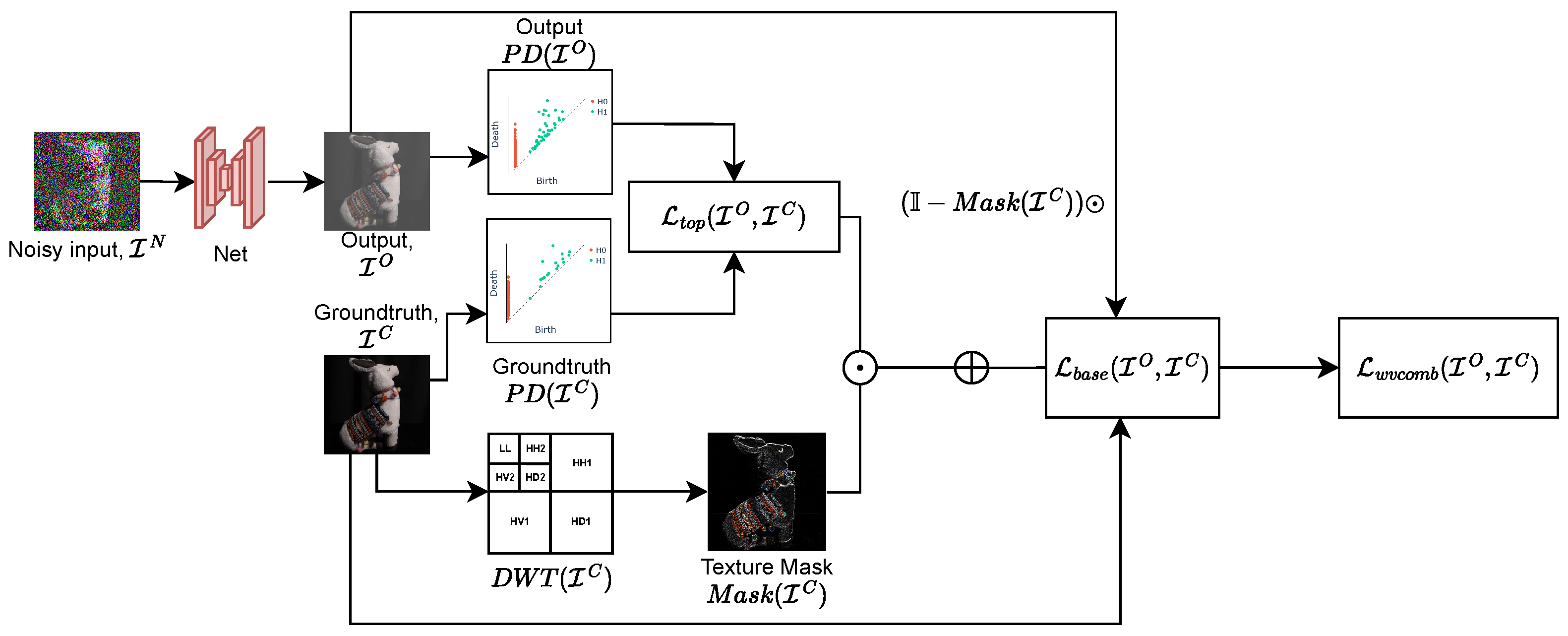
4. Wavelet-Based Topological Loss Function
4.1. Topological Loss Function
4.2. Texture Mask
| Algorithm 1: Wavelet Topological Image Denoising |
| Input: Noisy image , Groundtruth image , Trainable model Output: Optimised parameter set Step 1: Wavelet Decomposition; Perform wavelet decomposition on to obtain band wavelet coefficients; Step 2: Texture Mask Calculation; Calculate the texture mask; Step 3: Acquire model output ; Apply model to noisy image: Step 4: Persistence Diagram Calculation; Calculate the persistence diagrams and of and , respectively; Step 5: Topological Loss Term Calculation; Calculate the total persistence values and for and , respectively; Calculate the topological loss component : Step 6: Base Loss Term Calculation; Calculate the base loss component as the loss between and ; Step 7: Combined Loss Calculation; Calculate the pixelwise mask-weighted topological loss to enforce the topological guidance in textured areas: and in remaining “plain” areas tune it down: Calculate the combined wavelet loss as the (-weighted) sum of the mask-weighted losses with gain ; Step 8: Find the parameters of the network, minimising combined loss; return ; |
5. Experiments and Discussion
5.1. Dataset
5.2. Training
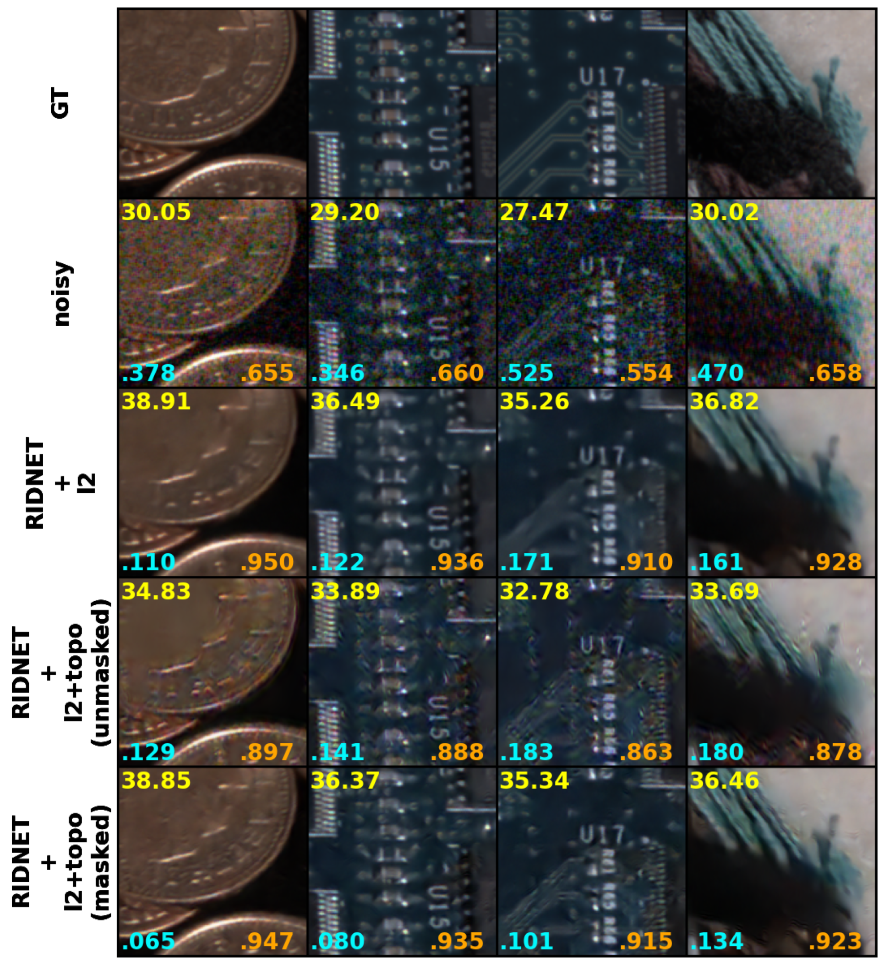
5.3. Results
6. Conclusions and Future Work
Supplementary Materials
Author Contributions
Funding
Institutional Review Board Statement
Informed Consent Statement
Data Availability Statement
Conflicts of Interest
References
- Buades, A.; Coll, B.; Morel, J.M. A non-local algorithm for image denoising. In Proceedings of the 2005 IEEE Computer Society Conference on Computer Vision and Pattern Recognition (CVPR’05), San Diego, CA, USA, 20–25 June 2005; Volume 2, pp. 60–65. [Google Scholar]
- Dabov, K.; Foi, A.; Katkovnik, V.; Egiazarian, K. BM3D image denoising with shape-adaptive principal component analysis. In Proceedings of the SPARS’09 Signal Processing with Adaptive Sparse Structured Representations, Saint-Malo, France, 6–9 April 2009. [Google Scholar]
- Anantrasirichai, N.; Bull, D. Artificial intelligence in the creative industries: A review. Artif. Intell. Rev. 2022, 55, 589–656. [Google Scholar]
- Krull, A.; Buchholz, T.O.; Jug, F. Noise2void-learning denoising from single noisy images. In Proceedings of the IEEE/CVF Conference on Computer Vision and Pattern Recognition, Long Beach, CA, USA, 16–17 June 2019; pp. 2129–2137. [Google Scholar]
- Batson, J.; Royer, L. Noise2self: Blind denoising by self-supervision. In Proceedings of the 36th International Conference on Machine Learning, Long Beach, CA, USA, 9–15 June 2019; pp. 524–533. [Google Scholar]
- Ulyanov, D.; Vedaldi, A.; Lempitsky, V. Deep image prior. In Proceedings of the 2018 IEEE/CVF Conference on Computer Vision and Pattern Recognition, Salt Lake City, UT, USA, 16 December 2018; pp. 9446–9454. [Google Scholar]
- Wang, Z.; Liu, J.; Li, G.; Han, H. Blind2Unblind: Self-Supervised Image Denoising With Visible Blind Spots. In Proceedings of the IEEE/CVF Conference on Computer Vision and Pattern Recognition (CVPR), New Orleans, LA, USA, 18–24 June 2022; pp. 2027–2036. [Google Scholar]
- Jang, H.; Park, J.; Jung, D.; Lew, J.; Bae, H.; Yoon, S. PUCA: Patch-Unshuffle and Channel Attention for Enhanced Self-Supervised Image Denoising. In Advances in Neural Information Processing Systems; Oh, A., Naumann, T., Globerson, A., Saenko, K., Hardt, M., Levine, S., Eds.; Curran Associates, Inc.: Red Hook, NY, USA, 2023; Volume 36, pp. 19217–19229. [Google Scholar]
- Anantrasirichai, N.; Bull, D. Contextual Colorization and Denoising for Low-Light Ultra High Resolution Sequences. In Proceedings of the 2021 IEEE International Conference on Image Processing (ICIP), Anchorage, AK, USA, 19–22 September 2021; pp. 1614–1618. [Google Scholar]
- Zhang, K.; Zuo, W.; Chen, Y.; Meng, D.; Zhang, L. Beyond a gaussian denoiser: Residual learning of deep cnn for image denoising. IEEE Trans. Image Process. 2017, 26, 3142–3155. [Google Scholar]
- Anwar, S.; Barnes, N. Real Image Denoising with Feature Attention. In Proceedings of the IEEE International Conference on Computer Vision (ICCV-Oral), Seoul, Republic of Korea, 27 October–2 November 2019. [Google Scholar]
- Abdelhamed, A.; Afifi, M.; Timofte, R.; Brown, M.S. NTIRE 2020 Challenge on Real Image Denoising: Dataset, Methods and Results. In Proceedings of the IEEE/CVF Conference on Computer Vision and Pattern Recognition (CVPR) Workshops, Seattle, WA, USA, 13–19 June 2020. [Google Scholar]
- Wu, W.; Liu, S.; Xia, Y.; Zhang, Y. Dual residual attention network for image denoising. Pattern Recognit. 2024, 149, 110291. [Google Scholar] [CrossRef]
- Jebur, R.S.; Zabil, M.H.B.M.; Hammood, D.A.; Cheng, L.K. A comprehensive review of image denoising in deep learning. Multimed. Tools Appl. 2024, 83, 58181–58199. [Google Scholar] [CrossRef]
- Malyugina, A.; Anantrasirichai, N.; Bull, D. A Topological Loss Function for Image Denoising on a new BVI-lowlight Dataset. Signal Process. 2023, 211, 109081. [Google Scholar] [CrossRef]
- Takeda, H.; Farsiu, S.; Milanfar, P. Kernel regression for image processing and reconstruction. IEEE Trans. Image Process. 2007, 16, 349–366. [Google Scholar]
- Wiener, N. Extrapolation, Interpolation and Smoothing of Stationary Time Series with Engineering Applications; The MIT Press: Cambridge, MA, USA, 1949. [Google Scholar]
- Tronicke, J.; Böniger, U. Steering kernel regression: An adaptive denoising tool to process GPR data. In Proceedings of the 2013 7th International Workshop on Advanced Ground Penetrating Radar, Nantes, France, 2–5 July 2013; pp. 1–4. [Google Scholar]
- Donoho, D.L.; Johnstone, J.M. Ideal spatial adaptation by wavelet shrinkage. Biometrika 1994, 81, 425–455. [Google Scholar]
- Chipman, H.A.; Kolaczyk, E.D.; McCulloch, R.E. Adaptive Bayesian wavelet shrinkage. J. Am. Stat. Assoc. 1997, 92, 1413–1421. [Google Scholar] [CrossRef]
- Shui, P.L. Image denoising using 2-D separable oversampled DFT modulated filter banks. IET Image Process. 2009, 3, 163–173. [Google Scholar] [CrossRef]
- Yu, G.; Sapiro, G. DCT image denoising: A simple and effective image denoising algorithm. Image Process. Line 2011, 1, 292–296. [Google Scholar]
- Foi, A.; Katkovnik, V.; Egiazarian, K. Pointwise shape-adaptive DCT for high-quality denoising and deblocking of grayscale and color images. IEEE Trans. Image Proc. 2007, 16, 1395–1411. [Google Scholar]
- Simoncelli, E.P.; Adelson, E.H. Noise removal via Bayesian wavelet coring. In Proceedings of the 3rd IEEE International Conference on Image Processing, Lausanne, Switzerland, 19 September 1996; Volume 1. [Google Scholar]
- Mihcak, M.K.; Kozintsev, I.; Ramchandran, K.; Moulin, P. Low-complexity image denoising based on statistical modeling of wavelet coefficients. IEEE Signal Process. Lett. 1999, 6, 300–303. [Google Scholar]
- Dabov, K.; Foi, A.; Katkovnik, V.; Egiazarian, K. Image denoising by sparse 3-D transform-domain collaborative filtering. IEEE Trans. Image Process. 2007, 16, 2080–2095. [Google Scholar]
- Dabov, K.; Foi, A.; Katkovnik, V.; Egiazarian, K. A Nonlocal and Shape-Adaptive Transform-Domain Collaborative Filtering. In Proceedings of the The 2008 International Workshop on Local and Non-Local Approximation in Image Processing, Lausanne, Switzerland, 23–24 August 2008. [Google Scholar]
- Aharon, M.; Elad, M.; Bruckstein, A. K-SVD: An algorithm for designing overcomplete dictionaries for sparse representation. IEEE Trans. Signal Process. 2006, 54, 4311. [Google Scholar]
- Chatterjee, P.; Milanfar, P. Clustering-based denoising with locally learned dictionaries. IEEE Trans. Image Process. 2009, 18, 1438–1451. [Google Scholar]
- Mairal, J.; Bach, F.; Ponce, J.; Sapiro, G.; Zisserman, A. Non-local sparse models for image restoration. In Proceedings of the 2009 IEEE 12th International Conference on Computer Vision, Kyoto, Japan, 29 September–2 October 2009; pp. 2272–2279. [Google Scholar]
- Fan, C.M.; Liu, T.J.; Liu, K.H. SUNet: Swin Transformer UNet for Image Denoising. In Proceedings of the 2022 IEEE International Symposium on Circuits and Systems (ISCAS), Austin, TX, USA, 27 May–1 June 2022; pp. 2333–2337. [Google Scholar] [CrossRef]
- Gurrola-Ramos, J.; Dalmau, O.; Alarcón, T.E. A Residual Dense U-Net Neural Network for Image Denoising. IEEE Access 2021, 9, 31742–31754. [Google Scholar] [CrossRef]
- Lehtinen, J.; Munkberg, J.; Hasselgren, J.; Laine, S.; Karras, T.; Aittala, M.; Aila, T. Noise2noise: Learning image restoration without clean data. arXiv 2018, arXiv:1803.04189. [Google Scholar]
- Byrne, N.; Clough, J.R.; Valverde, I.; Montana, G.; King, A.P. A Persistent Homology-Based Topological Loss for CNN-Based Multiclass Segmentation of CMR. IEEE Trans. Med. Imaging 2023, 42, 3–14. [Google Scholar] [CrossRef]
- Zomorodian, A.; Carlsson, G. Computing persistent homology. In Proceedings of the Twentieth Annual Symposium on Computational Geometry, Brooklyn, NY, USA, 8–11 June 2004. [Google Scholar]
- Edelsbrunner, H.; Letscher, D.; Zomorodian, A. Topological persistence and simplification. Discret. Comput. Geom. 2002, 28, 511–533. [Google Scholar]
- Epstein, C.; Carlsson, G.; Edelsbrunner, H. Topological data analysis. Inverse Probl. 2011, 27, 120201. [Google Scholar]
- Malyugina, A.; Anantrasirichai, N.; Bull, D. A Topological Loss Function: Image Denoising on a Low-Light Dataset. arXiv 2022, arXiv:2208.04573. [Google Scholar] [CrossRef]
- Carlsson, G.; Ishkhanov, T.; Silva, V.D.; Zomorodian, A. On the local behavior of spaces of natural images. Int. J. Comp. Vis. 2008, 76, 1–12. [Google Scholar] [CrossRef]
- Choe, S.; Ramanna, S. Cubical Homology-Based Machine Learning: An Application in Image Classification. Axioms 2022, 11, 112. [Google Scholar] [CrossRef]
- Anantrasirichai, N.; Burn, J.; Bull, D. Terrain Classification From Body-Mounted Cameras During Human Locomotion. IEEE Trans. Cybern. 2015, 45, 2249–2260. [Google Scholar] [CrossRef] [PubMed]
- Hill, P.; Anantrasirichai, N.; Achim, A.; Al-Mualla, M.; Bull, D. Undecimated Dual-Tree Complex Wavelet Transforms. Signal Process. Image Commun. 2015, 35, 61–70. [Google Scholar] [CrossRef]
- Schmidt, E. Zur Theorie der linearen und nichtlinearen Integralgleichungen. Math. Ann. 1907, 63, 433–476. [Google Scholar] [CrossRef]
- Anantrasirichai, N.; Burn, J.; Bull, D.R. Robust texture features based on undecimated dual-tree complex wavelets and local magnitude binary patterns. In Proceedings of the 2015 IEEE International Conference on Image Processing (ICIP), Quebec City, QC, Canada, 27–30 September 2015; pp. 3957–3961. [Google Scholar] [CrossRef]
- Malyugina, A.; Anantrasirichai, N.; Bull, D. BVI-LOWLIGHT, 2022. Available online: https://ieee-dataport.org/documents/bvi-lowlight-images (accessed on 30 October 2023).
- Ronneberger, O.; Fischer, P.; Brox, T. U-net: Convolutional networks for biomedical image segmentation. In Proceedings of the Medical Image Computing and Computer-Assisted Intervention—MICCAI 2015, Munich, Germany, 5–9 October 2015; Springer: Berlin/Heidelberg, Germany, 2015; pp. 234–241. [Google Scholar]
- Johnson, J.; Alahi, A.; Fei Fei, L. Perceptual Losses for Real-Time Style Transfer and Super-Resolution. arXiv 2016, arXiv:1603.08155. [Google Scholar] [CrossRef]
- Zhang, R.; Isola, P.; Efros, A.A.; Shechtman, E.; Wang, O. The Unreasonable Effectiveness of Deep Features as a Perceptual Metric. In Proceedings of the IEEE Conference on Computer Vision and Pattern Recognition, Salt Lake City, UT, USA, 18–23 June 2018. [Google Scholar]


| LPIPS | PSNR | SSIM | |
|---|---|---|---|
| Noisy | 0.430 | 29.19 | 0.632 |
| DnCNN+l1 | 0.172 | 35.26 | 0.918 |
| DnCNN+l1+vgg | 0.166 | 35.33 | 0.917 |
| DnCNN+l1+topo | 0.129 | 35.60 | 0.923 |
| DnCNN+l1+topo+vgg | 0.134 | 35.66 | 0.921 |
| DnCNN+l2 | 0.154 | 35.54 | 0.923 |
| DnCNN+l2+vgg | 0.186 | 34.83 | 0.914 |
| DnCNN+l2+topo | 0.131 | 35.42 | 0.918 |
| DnCNN+l2+topo+vgg | 0.124 | 35.55 | 0.919 |
| RIDNET+l1 | 0.119 | 36.97 | 0.934 |
| RIDNET+l1+vgg | 0.115 | 37.06 | 0.936 |
| RIDNET+l1+topo | 0.096 | 37.24 | 0.938 |
| RIDNET+l1+topo+vgg | 0.108 | 37.23 | 0.937 |
| RIDNET+l2 | 0.098 | 37.30 | 0.937 |
| RIDNET+l2+vgg | 0.098 | 37.23 | 0.939 |
| RIDNET+l2+topo | 0.094 | 36.65 | 0.928 |
| RIDNET+l2+topo+vgg | 0.089 | 36.91 | 0.933 |
| UNet+l1 | 0.180 | 35.36 | 0.916 |
| UNet+l1+vgg | 0.179 | 35.34 | 0.915 |
| UNet+l1+topo | 0.136 | 35.68 | 0.923 |
| UNet+l1+topo+vgg | 0.139 | 35.65 | 0.924 |
| UNet+l2 | 0.171 | 35.64 | 0.919 |
| UNet+l2+vgg | 0.165 | 35.75 | 0.922 |
| UNet+l2+topo | 0.121 | 35.82 | 0.919 |
| UNet+l2+topo+vgg | 0.116 | 35.88 | 0.923 |
Disclaimer/Publisher’s Note: The statements, opinions and data contained in all publications are solely those of the individual author(s) and contributor(s) and not of MDPI and/or the editor(s). MDPI and/or the editor(s) disclaim responsibility for any injury to people or property resulting from any ideas, methods, instructions or products referred to in the content. |
© 2025 by the authors. Licensee MDPI, Basel, Switzerland. This article is an open access article distributed under the terms and conditions of the Creative Commons Attribution (CC BY) license (https://creativecommons.org/licenses/by/4.0/).
Share and Cite
Malyugina, A.; Anantrasirichai, N.; Bull, D. Wavelet-Based Topological Loss for Low-Light Image Denoising. Sensors 2025, 25, 2047. https://doi.org/10.3390/s25072047
Malyugina A, Anantrasirichai N, Bull D. Wavelet-Based Topological Loss for Low-Light Image Denoising. Sensors. 2025; 25(7):2047. https://doi.org/10.3390/s25072047
Chicago/Turabian StyleMalyugina, Alexandra, Nantheera Anantrasirichai, and David Bull. 2025. "Wavelet-Based Topological Loss for Low-Light Image Denoising" Sensors 25, no. 7: 2047. https://doi.org/10.3390/s25072047
APA StyleMalyugina, A., Anantrasirichai, N., & Bull, D. (2025). Wavelet-Based Topological Loss for Low-Light Image Denoising. Sensors, 25(7), 2047. https://doi.org/10.3390/s25072047