
Projection Profiling: A Data Compressing Strategy in Three-Dimensional Liquid Chromatography for Quality Control of Traditional Herbal Medicine

Abstract
1. Introduction
2. Theory
2.1. Baseline Correction
2.2. Peak Detection and Peak Integration
2.3. Similarity Analysis
3. Materials and Methods
3.1. Materials and Reagents
3.2. Standards and Sample Preparation
3.3. HPLC Analysis
4. Results and Discussion
4.1. Effects of Wavelength and Integration on Analytical Method Validation
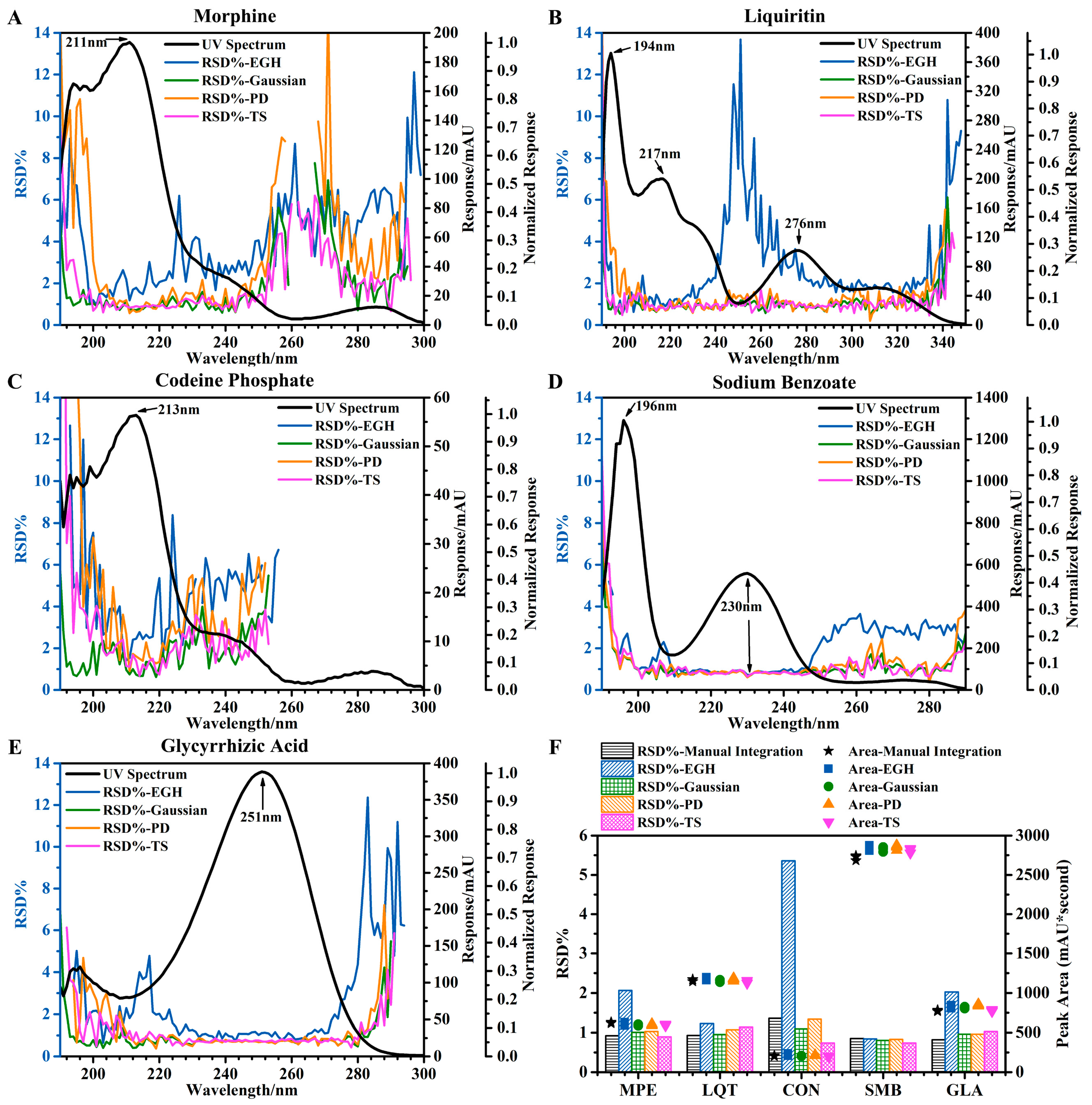
4.1.1. Precision (Repeatability)
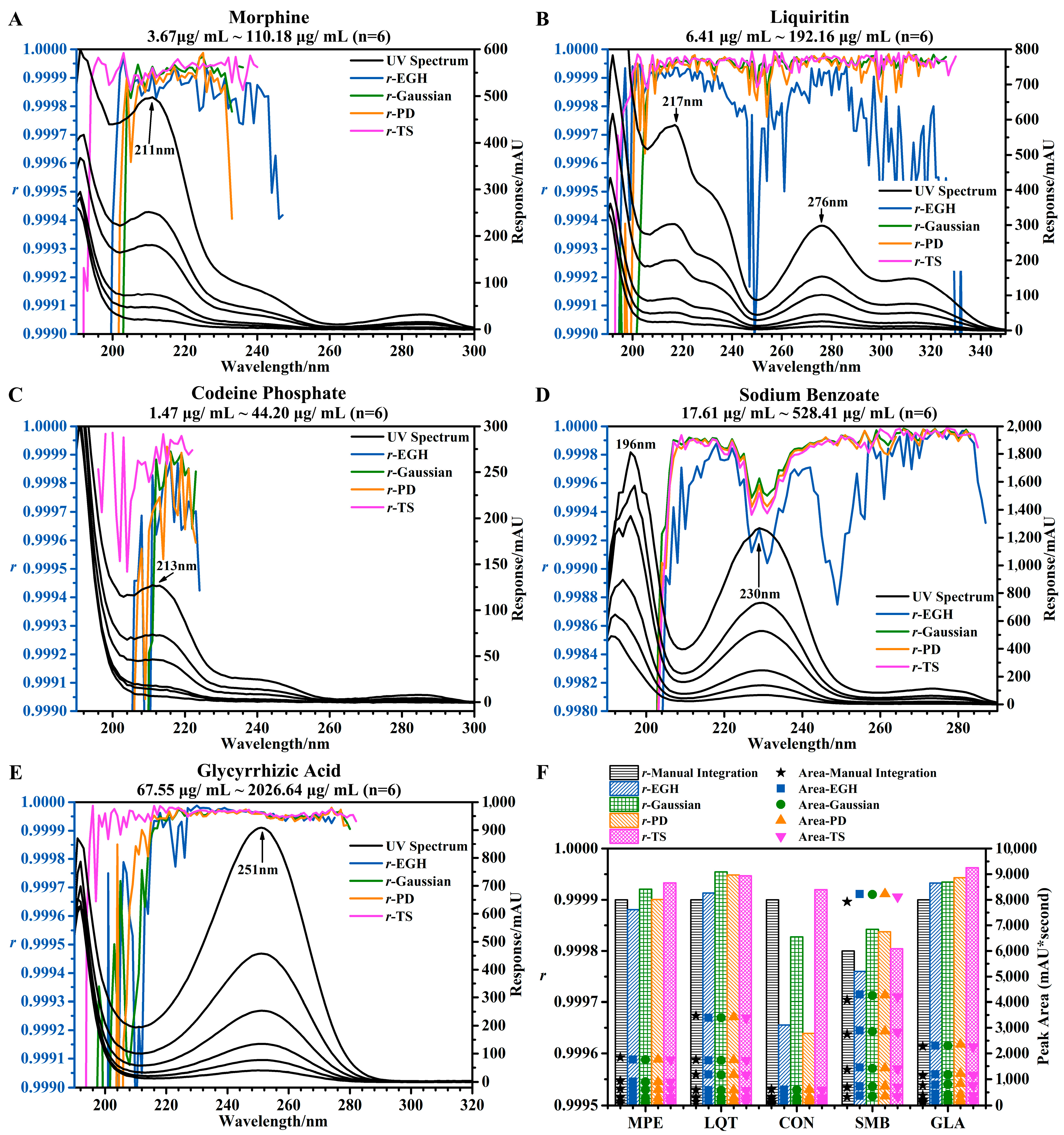
4.1.2. Linearity
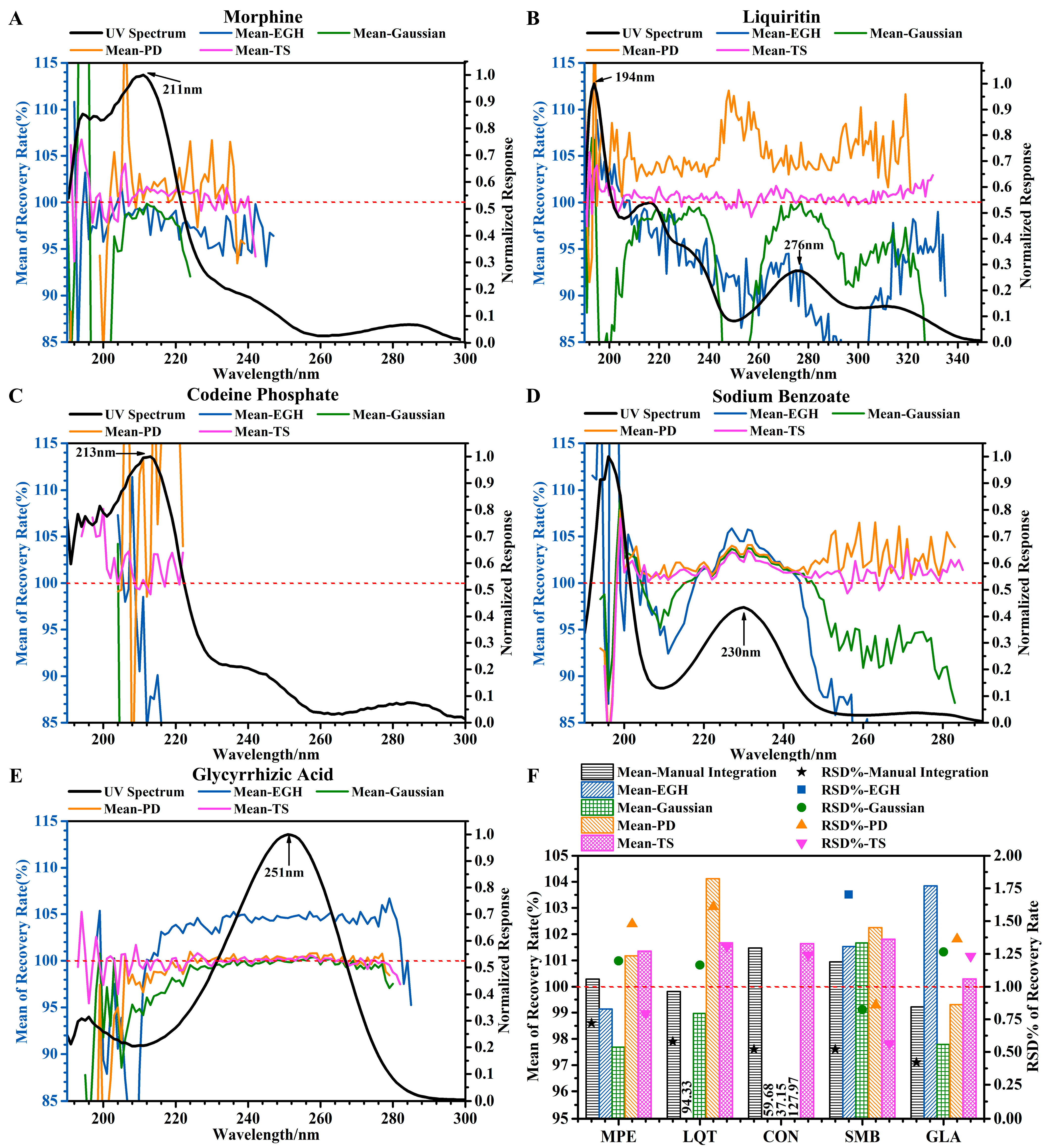
4.1.3. Accuracy
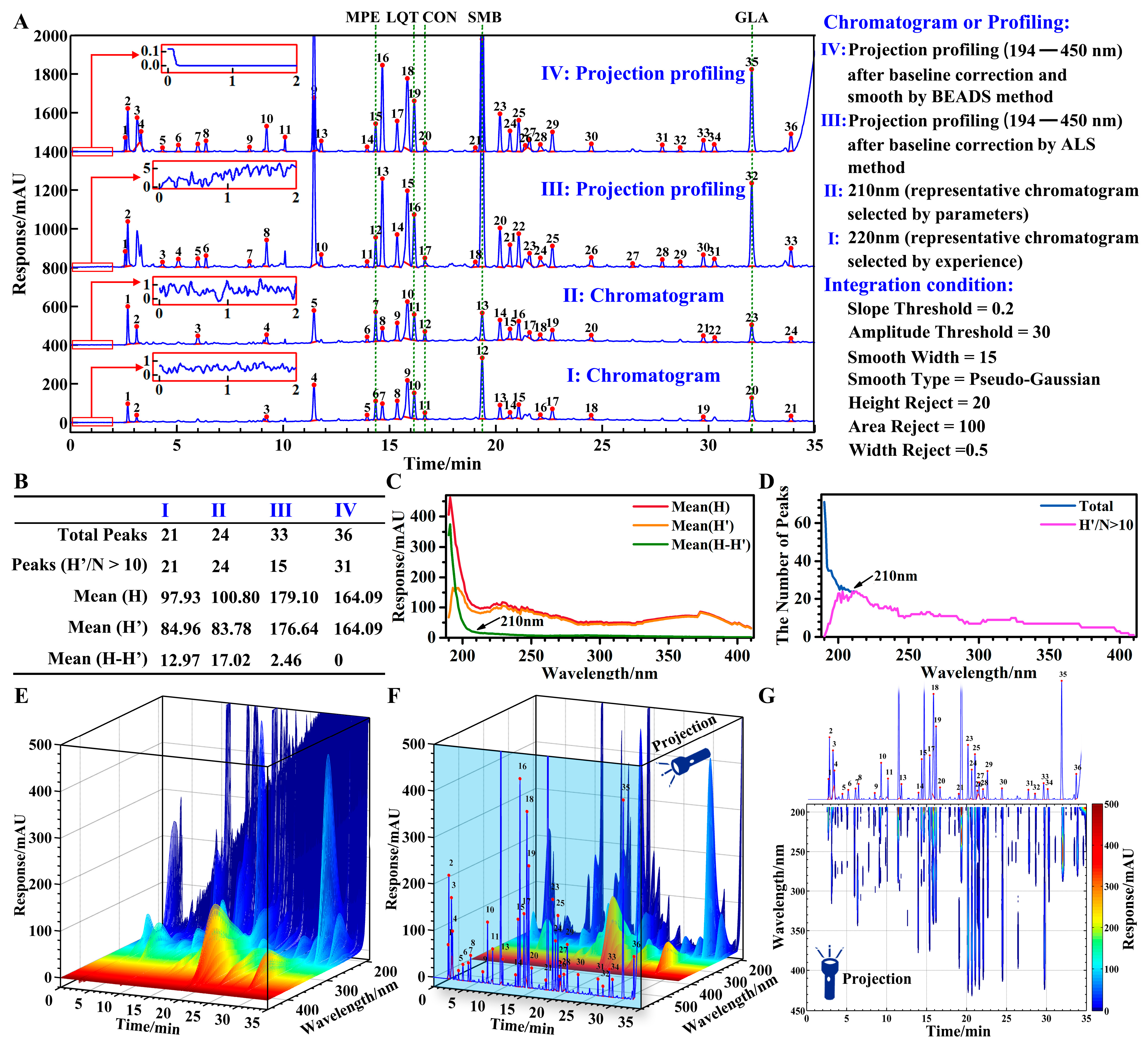
4.2. Chromatogram vs. Projection Profiling
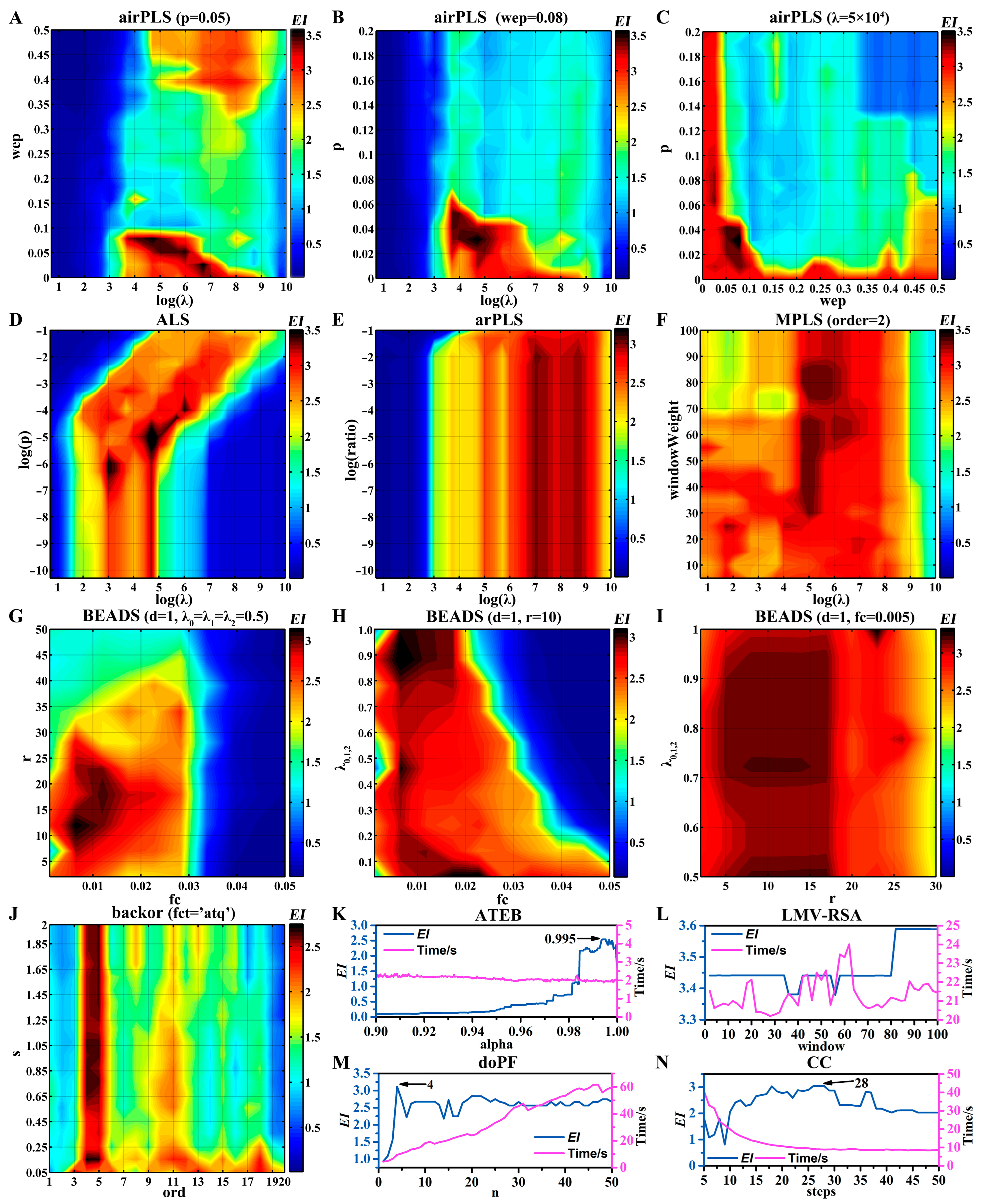
4.3. Baseline Correction
- A reduction in baseline noise results in a higher PN, approaching PALL, while a larger AN indicates greater proximity to AALL.
- Lower baseline drift leads to a higher PD, approaching PALL, while a larger AD suggests a closer proximity to AALL.
- Fewer distorted peaks lead to a smaller PB, approaching zero. When PB equals zero, the overfitting of the baseline is absent.
- Since projection profiling does not modify the original data, when PB equals zero, a larger AALL implies higher chromatographic accuracy.
- The EI value ranges from 0 to 4, with a higher EI indicating better baseline correction and more accurate quantitative analysis results. When EI equals 4, optimal baseline correction is achieved, accompanied by the highest chromatographic accuracy and reproducibility.
- Different baseline correction algorithms are founded on distinct principles and exhibit their respective advantages and disadvantages. Identical EI values can result in entirely different corrected baselines and projection profiles (or chromatograms). Therefore, when comparing different baseline correction algorithms, a higher EI does not necessarily correlate with improved chromatographic accuracy and reproducibility.
- EI can be used to compare different baseline correction algorithms and optimize parameters within a single algorithm. However, it is directly proportional only to the effectiveness of baseline correction and is correlated, but not directly proportional to chromatographic accuracy and reproducibility.
4.4. Effects of Wavelength on Similarity Analyses
5. Conclusions
Supplementary Materials
Funding
Institutional Review Board Statement
Informed Consent Statement
Data Availability Statement
Acknowledgments
Conflicts of Interest
Abbreviations
| airPLS | Adaptive iteratively reweighted penalized least squares |
| ALS | Asymmetric least squares |
| ANOVA | Analysis of variance |
| arPLS | asymmetrically reweighted penalized least squares |
| ATEB | Automatic two-side exponential baseline correction algorithm |
| backcor | Background correction by minimizing a non-quadratic cost function |
| BEADS | Baseline estimation and denoising with sparsity |
| CC | Corner-cutting |
| CLT | Compound licorice tablet |
| CON | Codeine |
| DAD | Diode array detector |
| EGH | Exponential-Gaussian hybrid |
| EI | Effective information |
| EMG | Exponentially modified Gaussian |
| GDCE | Generic drug consistency evaluation |
| HPLC | High-performance liquid chromatography |
| LMV-RSA | Local minimum values coupled with robust statistical analysis |
| LQT | Liquiritin |
| MPE | Morphine |
| MPLS | Morphologically weighted penalized least squares |
| PD | Perpendicular drop |
| PF | Polynomial fitting |
| RFP | Reference fingerprint |
| RSD | Relative standard deviation |
| SFP | Sample fingerprint |
| SMB | Sodium benzoate |
| SWiMA | Small-window moving average automated baseline correction |
| TS | Tangent skim |
| THM | Traditional herbal medicine |
References
- Li, Y.; Fan, J.; Jin, H.; Wei, F.; Ma, S. New vision for TCM quality control: Elemental fingerprints and key ingredient combination strategy for identification and evaluation of TCMs. Eur. J. Med. Chem. 2025, 281, 117006. [Google Scholar] [CrossRef] [PubMed]
- National Pharmacopoeia Commission. Pharmacopoeia of the People’s Republic of China: Volume II. Beijing; China Medical Science and Technology Press: Beijing, China, 2005; pp. 796–798. [Google Scholar]
- Park, Y.S.; Kang, S.M.; Kim, Y.J.; Lee, I.J. Exploring the dietary and therapeutic potential of licorice (Glycyrrhiza uralensis Fisch.) sprouts. J. Ethnopharmacol. 2024, 328, 118101. [Google Scholar] [CrossRef] [PubMed]
- Chen, Q.-H.; Zhou, Z.-Y.; Feng, M.-T.; He, J.-H.; Xu, Y.-Q.; Liao, B.-K. Unraveling the inhibitive performance and adsorption behavior of expired compound glycyrrhizin tablets as an eco-friendly corrosion inhibitor for copper in acidic medium. J. Taiwan Inst. Chem. Eng. 2025, 168, 105913. [Google Scholar] [CrossRef]
- Luo, Y.; Yang, H.; Tao, G. Systematic review on fingerprinting development to determine adulteration of Chinese herbal medicines. Phytomedicine 2024, 129, 155667. [Google Scholar] [CrossRef]
- Zhang, J.; Chen, S.; Sun, G. Spectral and chromatographic overall analysis: An insight into chemical equivalence assessment of traditional Chinese medicine. J. Chromatogr. A 2020, 1610, 460556. [Google Scholar] [CrossRef] [PubMed]
- Zhang, M.; Sun, J.; Chen, P. FlavonQ: An automated data processing tool for profiling flavone and flavonol glycosides with ultra-high-performance liquid chromatography-diode array detection-high resolution accurate mass-mass spectrometry. Anal. Chem. 2015, 87, 9974–9981. [Google Scholar] [CrossRef]
- Stevenson, P.G.; Conlan, X.A.; Barnett, N.W. Evaluation of the asymmetric least squares baseline algorithm through the accuracy of statistical peak moments. J. Chromatogr. A 2013, 1284, 107–111. [Google Scholar] [CrossRef]
- Zhang, Z.M.; Chen, S.; Liang, Y.Z. Baseline correction using adaptive iteratively reweighted penalized least squares. Analyst 2010, 135, 1138–1146. [Google Scholar] [CrossRef]
- Eilers, P.H.; Boelens, H.F. Baseline Correction with Asymmetric Least Squares Smoothing. Leiden Univ. Med. Cent. Rep. 2005, 1, 5. Available online: https://prod-dcd-datasets-public-files-eu-west-1.s3.eu-west-1.amazonaws.com/dd7c1919-302c-4ba0-8f88-8aa61e86bb9d (accessed on 11 March 2025).
- Baek, S.-J.; Park, A.; Ahn, Y.-J.; Choo, J. Baseline correction using asymmetrically reweighted penalized least squares smoothing. Analyst 2015, 140, 250–257. [Google Scholar] [CrossRef]
- Liu, X.; Zhang, Z.; Liang, Y.; Sousa, P.F.M.; Yun, Y.; Yu, L. Baseline correction of high resolution spectral profile data based on exponential smoothing. Chemom. Intell. Lab. Syst. 2014, 139, 97–108. [Google Scholar] [CrossRef]
- Mazet, V.; Carteret, C.; Brie, D.; Idier, J.; Humbert, B. Background removal from spectra by designing and minimising a non-quadratic cost function. Chemom. Intell. Lab. Syst. 2005, 76, 121–133. [Google Scholar] [CrossRef]
- Ning, X.; Selesnick, I.W.; Duval, L. Chromatogram baseline estimation and denoising using sparsity (BEADS). Chemom. Intell. Lab. Syst. 2014, 139, 156–167. [Google Scholar] [CrossRef]
- Liu, Y.J.; Zhou, X.G.; Yu, Y.D. A Concise Iterative Method with Bezier Technique for Baseline Construction. Analyst 2013, 140, 7984–7996. [Google Scholar] [CrossRef] [PubMed]
- Mani-Varnosfaderani, A.; Kanginejad, A.; Gilany, K.; Valadkhani, A. Estimating complicated baselines in analytical signals using the iterative training of Bayesian regularized artificial neural networks. Anal. Chim. Acta 2016, 940, 56–64. [Google Scholar] [CrossRef]
- Fu, H.Y.; Li, H.D.; Yu, Y.J.; Wang, B.; Lu, P.; Cui, H.P.; Liu, P.P.; She, Y.B. Simple automatic strategy for background drift correction in chromatographic data analysis. J. Chromatogr. A 2016, 1449, 89–99. [Google Scholar] [CrossRef]
- Li, Z.; Zhan, D.J.; Wang, J.J.; Huang, J.; Xu, Q.S.; Zhang, Z.M.; Zheng, Y.B.; Liang, Y.Z.; Wang, H. Morphological weighted penalized least squares for background correction. Analyst 2013, 138, 4483–4492. [Google Scholar] [CrossRef]
- Schulze, H.G.; Foist, R.B.; Okuda, K.; Ivanov, A.; Turner, R.F. A small-window moving average-based fully automated baseline estimation method for Raman spectra. Appl. Spectrosc. 2012, 66, 757–764. [Google Scholar] [CrossRef]
- Prakash, B.D.; Wei, Y.C. A fully automated iterative moving averaging (AIMA) technique for baseline correction. Analyst 2011, 136, 3130–3135. [Google Scholar] [CrossRef]
- Lan, K.; Jorgenson, J.W. A hybrid of exponential and gaussian functions as a simple model of asymmetric chromatographic peaks. J. Chromatogr. A 2001, 915, 1–13. [Google Scholar] [CrossRef]
- Johnsen, L.G.; Skov, T.; Houlberg, U.; Bro, R. An automated method for baseline correction, peak finding and peak grouping in chromatographic data. Analyst 2013, 138, 3502. [Google Scholar] [CrossRef] [PubMed]
- Whittaker, E.T. On a new method of graduation. Proc. Edinb. Math. Soc. 1992, 41, 63–75. [Google Scholar] [CrossRef]
- Eilers, P.H.C. A Perfect Smoother. Anal. Chem. 2003, 75, 3631–3636. [Google Scholar] [CrossRef] [PubMed]
- Eilers, P.H.C. Parametric Time Warping. Anal. Chem. 2004, 76, 404–411. [Google Scholar] [CrossRef]
- Erny, G.L.; Acunha, T.; Simó, C.; Cifuentes, A.; Alves, A. Finnee—A Matlab toolbox for separation techniques hyphenated high resolution mass spectrometry dataset. Chemom. Intell. Lab. Syst. 2016, 155, 138–144. [Google Scholar] [CrossRef]
- Zhang, J.; Sun, G. Assessment of quality consistency in traditional Chinese medicine using multi-wavelength fusion profiling by integrated quantitative fingerprint method: Niuhuang Jiedu pill as an example. J. Sep. Sci. 2019, 42, 509–521. [Google Scholar] [CrossRef]
- Devos, O.; Mouton, N.; Sliwa, M.; Ruckebusch, C. Baseline correction methods to deal with artifacts in femtosecond transient absorption spectroscopy. Anal. Chim. Acta 2011, 705, 64–71. [Google Scholar] [CrossRef]


| Baseline Correction Algorithms | Abbr. | Parameters a | Ref. | Open-Source ((Accessed on 13 March 2025)) |
|---|---|---|---|---|
| Adaptive iteratively reweighted penalized least squares | airPLS | lambda (λ, smoothness) I, order (order of differences) II, wep (weight) I, p (asymmetry) I, itermax (maximum iteration times) II | [9] | https://github.com/zmzhang/airPLS |
| Asymmetric least squares | ALS | lambda (λ, smoothness) I, p (asymmetry) I | [10] | https://github.com/chemplexity/chromatography/blob/master/Development/Parallel%20Computing/ParallelBaseline.m (parallel computing) |
| Asymmetrically reweighted penalized least squares | arPLS | lambda (λ, smoothness) I, ratio (termination condition) I | [11] | [11] |
| Automatic two-side exponential baseline correction algorithm | ATEB | alpha (α, smoothing factor) I | [12] | [12] Supplementary Materials |
| Background correction by minimizing a non-quadratic cost function | backcor | ord (the polynomial order) I, s (the threshold of the cost function) I, fct (cost functions) II | [13] | https://www.mathworks.com/matlabcentral/fileexchange/27429-background-correction?s_tid=FX_rc2_behav |
| Baseline estimation and denoising with sparsity | BEADS | d (filter order) II, fc (filter cut-off frequency) I, r (asymmetry ratio) I, lambdai (λi, i = 0, 1, 2, regularization parameters) II | [14] | https://www.mathworks.com/matlabcentral/fileexchange/49974-beads-baseline-estimation-and-denoising-with-sparsity?s_tid=FX_rc3_behav |
| A variant of polynomial fitting | doPF | n (order of the polynomial) II | None | https://github.com/glerny/Finnee2016/blob/master/List%20of%20Functions/Baseline%20corrections/doPF.m |
| Corner-Cutting | CC | steps (number of iterations) II | [15] | [16] Supplementary Materials |
| Local minimum values coupled with robust statistical analysis | LMV-RSA | w (window width) II | [17] | [17] Supplementary Materials |
| Morphologically weighted penalized least squares | MPLS | lambda (λ, smoothness) I, window weight (half the window width of the structuring element) I, order (order of differences) II, | [18] | https://code.google.com/archive/p/mpls/downloads |
| Small-window moving average automated baseline correction | SWiMA | NO parameters | [19] | https://www.mathworks.com/matlabcentral/fileexchange/69649-raman-spectrum-baseline-removal?s_tid=srchtitle |
| Baseline Correction Algorithms | The Number of Optimizations | Total Execution Time (s) | Execution Time per Optimization (s) a | EI Value Under Optimal Conditions | PALL | Fluctuation of Baseline Noise (mAU) b | Optimal Conditions |
|---|---|---|---|---|---|---|---|
| airPLS | 20 × 20 × 3 = 1200 | 11,604.4 | 9.67 | 3.19 | 31 | 1–5 | lambda = 5 × 10⁴, order = 2, wep = 0.08, p = 0.03, iterate = 20 |
| ALS | 20 × 20 = 400 | 1138.3 | 2.8 | 3.61 | 33 | 2–5 | lambda = 5 × 10⁴, p = 5 × 10⁻⁶ |
| arPLS | 20 × 20 = 400 | 3719.3 | 9.3 | 3.02 | 30 | 0–2 | lambda = 107, ratio = 10−2 |
| ATEB | 400 | 848.7 | 2.1 | 2.54 | 25 | 0.1–0.4 | alpha = 0.995 |
| backor | 20 × 20 = 400 | 925.4 | 2.3 | 2.72 | 28 | 0–0.5 | ord = 4, s = 0.15, fct = ‘atq’ |
| BEADS | 10 × 10 × 3 = 300 | 18,043.2 | 60.1 | 3.19 | 30 | 0–0.8 | d = 1, fc = 0.005, r = 10, lam0 = lam1 = lam2 = 0.7 |
| CC | 45 | 562.6 | 12.5 | 3.01 | 26 | 2–6 | steps = 28 |
| doPF | 50 | 1740.5 | 34.8 | 3.11 | 29 | 0–2 | n = 4 |
| LMV-RSA | 50 | 1067.1 | 21.3 | 3.59 | 30 | 0–3.5 | window = 100 |
| MPLS | 20 × 20 = 400 | 6756.3 | 16.9 | 3.34 | 32 | 1–4 | lambda = 105, windowWeight = 40, order = 2 |
| Type III Sum of Squares | Degrees of Freedom | Mean Square | F Value | Significance | |
|---|---|---|---|---|---|
| Corrected Model | 0.935 a | 54 | 0.017 | 13.698 | 0.000 |
| Intercept | 3966.296 | 1 | 3966.2 | 3,138,971.4 | 0.000 |
| Sample Number | 0.698 | 32 | 0.022 | 17.251 | 0.000 |
| Wavelengths b | 0.132 | 19 | 0.007 | 5.508 | 0.000 |
| Similarity Methods c | 0.000 | 2 | 0.000 | 0.187 | 0.829 |
| Quality or Quantity c | 0.104 | 1 | 0.104 | 82.655 | 0.000 |
| Error | 4.934 | 3905 | 0.001 | ||
| Total | 3972.165 | 3960 | |||
| Corrected Total | 5.869 | 3959 |
| Type III Sum of Squares | Degrees of Freedom | Mean Square | F Value | Significance | |
|---|---|---|---|---|---|
| Corrected Model | 0.048 a | 36 | 0.001 | 7.437 | 0.000 |
| Intercept | 397.937 | 1 | 397.9 | 2,210,895.3 | 0.000 |
| Sample Number | 0.042 | 32 | 0.001 | 7.359 | 0.000 |
| Chromatography in 210 nm or Projection Profiling b | 4.235 × 10⁻⁵ | 1 | 4.235 × 10⁻⁵ | 0.235 | 0.628 |
| Similarity Methods c | 1.225 × 10⁻⁵ | 2 | 6.127 × 10⁻⁶ | 0.034 | 0.967 |
| Quality or Quantity c | 0.006 | 1 | 0.006 | 31.945 | 0.000 |
| Error | 0.065 | 359 | 0.000 | ||
| Total | 398.050 | 396 | |||
| Corrected Total | 0.113 | 395 |
Disclaimer/Publisher’s Note: The statements, opinions and data contained in all publications are solely those of the individual author(s) and contributor(s) and not of MDPI and/or the editor(s). MDPI and/or the editor(s) disclaim responsibility for any injury to people or property resulting from any ideas, methods, instructions or products referred to in the content. |
© 2025 by the author. Licensee MDPI, Basel, Switzerland. This article is an open access article distributed under the terms and conditions of the Creative Commons Attribution (CC BY) license (https://creativecommons.org/licenses/by/4.0/).
Share and Cite
Zhang, J. Projection Profiling: A Data Compressing Strategy in Three-Dimensional Liquid Chromatography for Quality Control of Traditional Herbal Medicine. Sensors 2025, 25, 2015. https://doi.org/10.3390/s25072015
Zhang J. Projection Profiling: A Data Compressing Strategy in Three-Dimensional Liquid Chromatography for Quality Control of Traditional Herbal Medicine. Sensors. 2025; 25(7):2015. https://doi.org/10.3390/s25072015
Chicago/Turabian StyleZhang, Jing. 2025. "Projection Profiling: A Data Compressing Strategy in Three-Dimensional Liquid Chromatography for Quality Control of Traditional Herbal Medicine" Sensors 25, no. 7: 2015. https://doi.org/10.3390/s25072015
APA StyleZhang, J. (2025). Projection Profiling: A Data Compressing Strategy in Three-Dimensional Liquid Chromatography for Quality Control of Traditional Herbal Medicine. Sensors, 25(7), 2015. https://doi.org/10.3390/s25072015