
Energy Loss Reduction for Distribution Electric Power Systems with Renewable Power Sources, Reactive Power Compensators, and Electric Vehicle Charge Stations

Abstract
1. Introduction
1.1. Motivation
1.2. Literature Review
- (1)
- Minimizing the overall active power loss;
- (2)
- Minimizing the total capacity of all renewable power sources;
- (3)
- Minimizing the total voltage deviation index.
- -
- Apply newly published meta-heuristic algorithms, which were recently published: the purpose is to find the most suitable algorithm for the problem;
- -
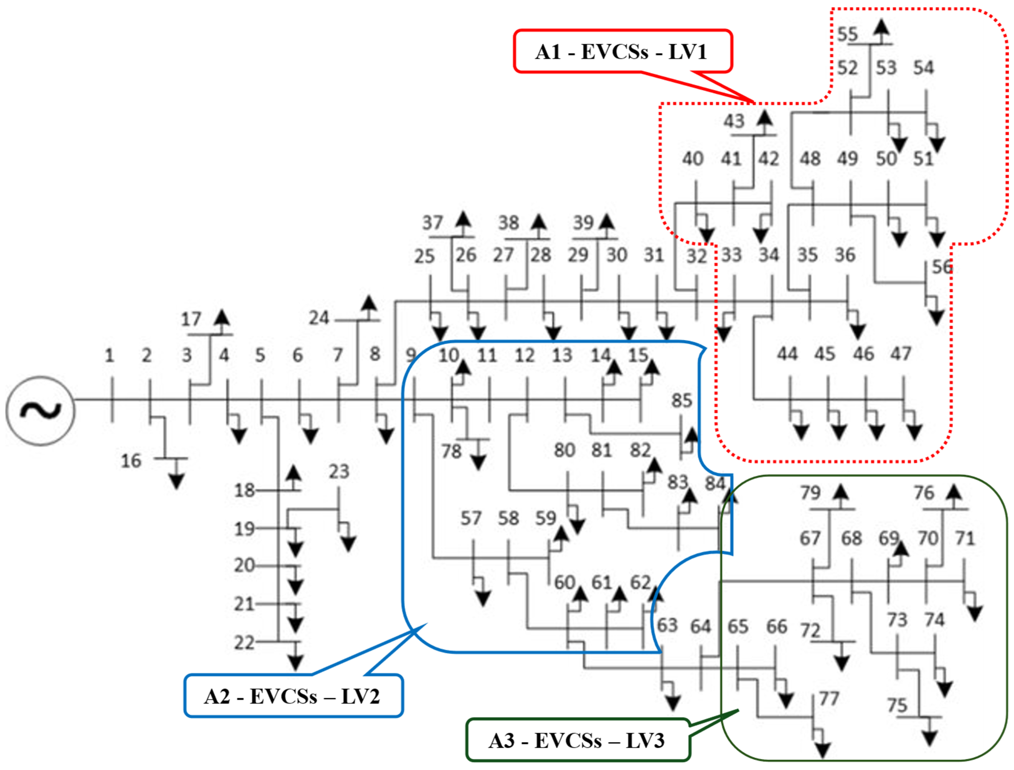
- Classify different zones in distribution electric power systems to install EVCSs: A group of distribution lines is selected to install several levels of EVCSs. The purpose is not to install many EVCSs close together;
- -
- Implement different penetration levels of EVCSs, with 25%, 50%, 75%, and 100%, in distribution electric power systems: the purpose is to survey the operating limits of the grids to avoid low voltage for base loads;
- -
- Implement the installation of capacitors in the distribution electric power systems corresponding to the different levels of EVCSs: the purpose is to enhance the operation limits of the grids with a low investment cost for installing capacitors;
- -
- Implement the installation of photovoltaic systems in distribution electric power systems corresponding to the different levels of EVCSs: the purpose is to enhance the operation limits of the grids with a higher investment cost for installing photovoltaic systems than capacitors;
- -
- Combine the simultaneous placement of capacitors and photovoltaic systems in distribution electric power systems: the use of both reactive and active power sources can improve voltage and reduce energy loss.
- -
- Determining the most effective meta-heuristic algorithm to find the optimal solution for each case study considered across all four scenarios implemented in the research;
- -
- Selecting the best penetration level of EVCSs in distribution electric power systems that can support electric vehicles highly and stabilize the operation of the distribution of electric power systems;
- -
- Selecting the most suitable power of capacitors for each penetration level of EVCSs: If capacitors can compensate for the voltage drop, their most optimal capacity is selected. In some cases, with very high penetration levels of EVCSs, capacitors cannot compensate for enough reactive power, and the grid is warned not to install more EVCSs;
- -
- Selecting the most suitable power of photovoltaic systems for each penetration level of EVCSs: For all cases with very high penetration levels of EVCSs, the system can compensate enough active power for the grid to still work stably and effectively; however, the high power of the systems can lead to high investment costs;
- -
- Using the simultaneous placement of capacitors and photovoltaic systems is very good for keeping voltage in a stable operation range, and the cost is more suitable than the use of only photovoltaic systems.
2. Problem Description
2.1. The Objective Function Considered
2.2. The Constraint Involved
- Power balance constraints: These constraints focus on ensuring the dynamic balance of the DEPS, which is represented by the correspondence between the total supplied power and the total demanded power with the loss amount. The constraints are applied for both active and reactive power, as shown by the following expressions:
- Operational voltage constraint: Voltage is a crucial factor that directly affects the operational status of all the electrical devices connected to the grid. Therefore, the voltage must be maintained in an allowed range between the minimum and maximum values to ensure the reliability and stability of a particular DEPS [30,31]. The constraint must meet the inequality below:
- Thermal constraint: This constraint mainly concerns the current amplitude circulated through a particular branch, which must be lower than the allowed value. Unlike voltage, the current amplitude needs to respect the maximum value only, as given in the expression below:
- Operating constraint of installed PV systems: This constraint means that PVs can inject a particular amount of active power into the grid within their minimum and maximum limits as described by the following equation:
- SC’s operational constraints: Similar to PV systems, the amount of reactive power supplied by SCs can only vary in an interval between the minimum and maximum bounds as follows:In addition, the total reactive power supplied by all capacitor banks must be lower or equal to the demands of loads and loss in lines, as expressed in the following inequality:
- Location constraints of PV systems: This constraint indicates that the placements of installed PV systems must satisfy the geography constraint. In the study, PV systems can be placed wherever, excluding the slack node, as shown in the following model:
- Location constraints of EVCSs: The study supposes that EVCSs are limited to the installed locations. This means that the EVCSs can be found in some feeders and not in others. The assumption is due to the difference of residences on different roads. Typically, EVCSs are really necessary for centers and not for rural areas. Thus, the locations of EVCSs are constrained by the following model:
3. The Applied Algorithm
3.1. Chameleon Swarm Algorithm
3.1.1. The Initialization
3.1.2. The Evaluation
3.1.3. The Update Process
- Stage 1: Seeking and detecting.
- Stage 2: Maneuvering and attacking.
3.1.4. The Boundary Check
3.1.5. The Refining Procedure
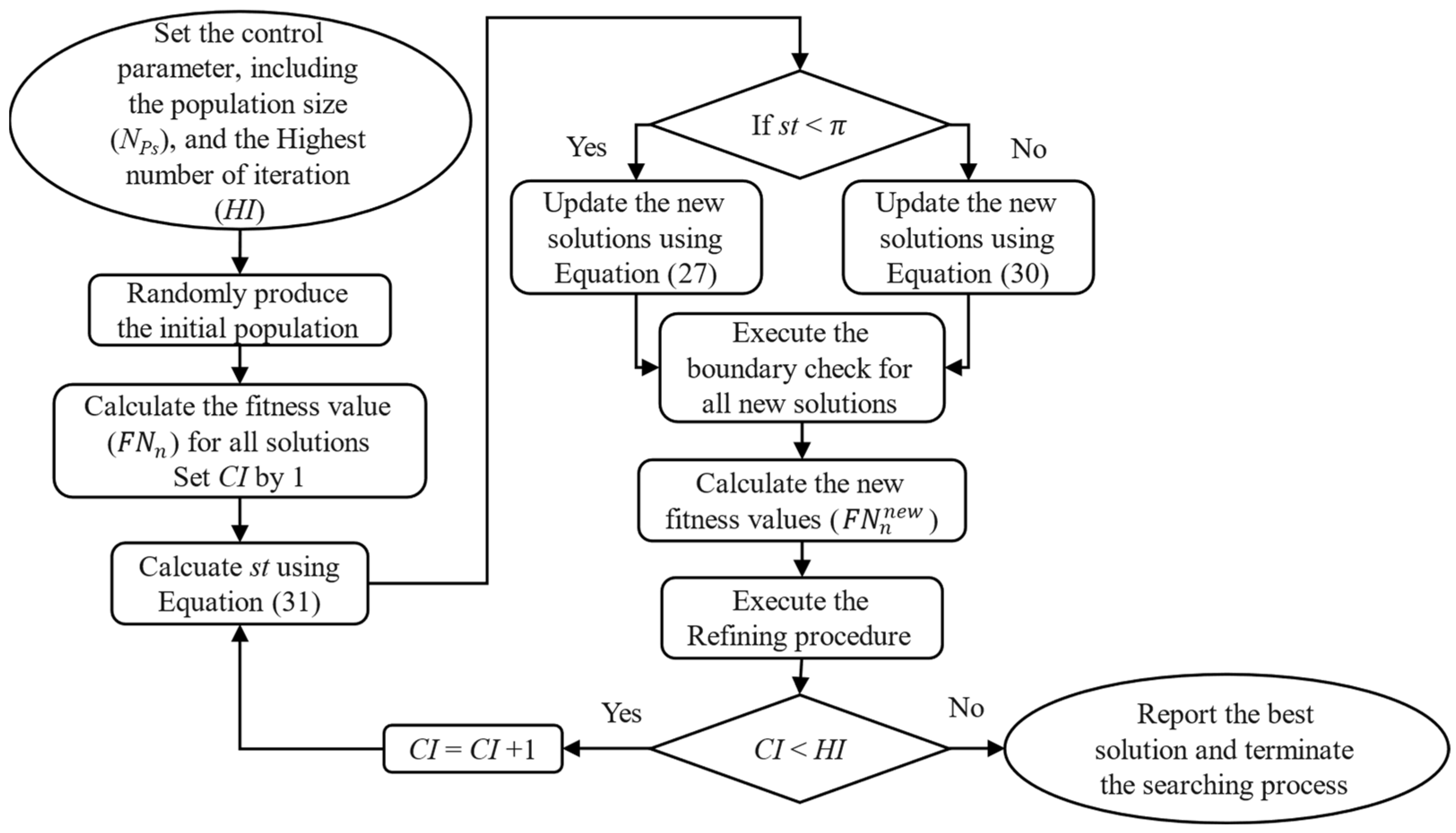
3.2. Snow Geese Algorithm
- Stage 1: The herringbone method
- Stage 2: The straight-line method
| If st < Executing the update process mentioned in Stage 1, Otherwise Executing the update process mentioned in Stage 2, End. |
4. Results
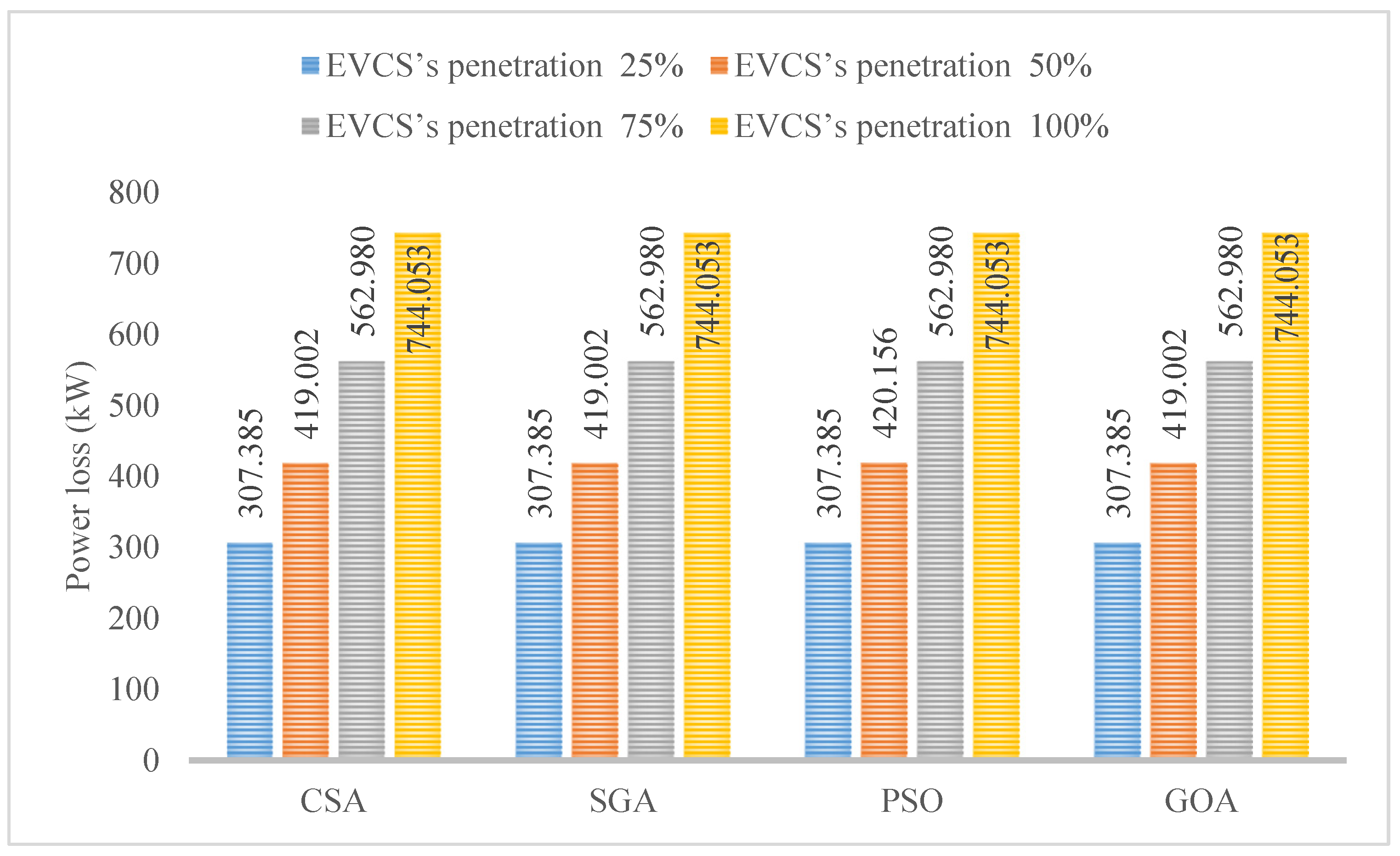
4.1. The Results Obtained in Scenario 1
4.2. The Results Obtained in the Second Scenario
4.2.1. The Results Obtained in Case 1
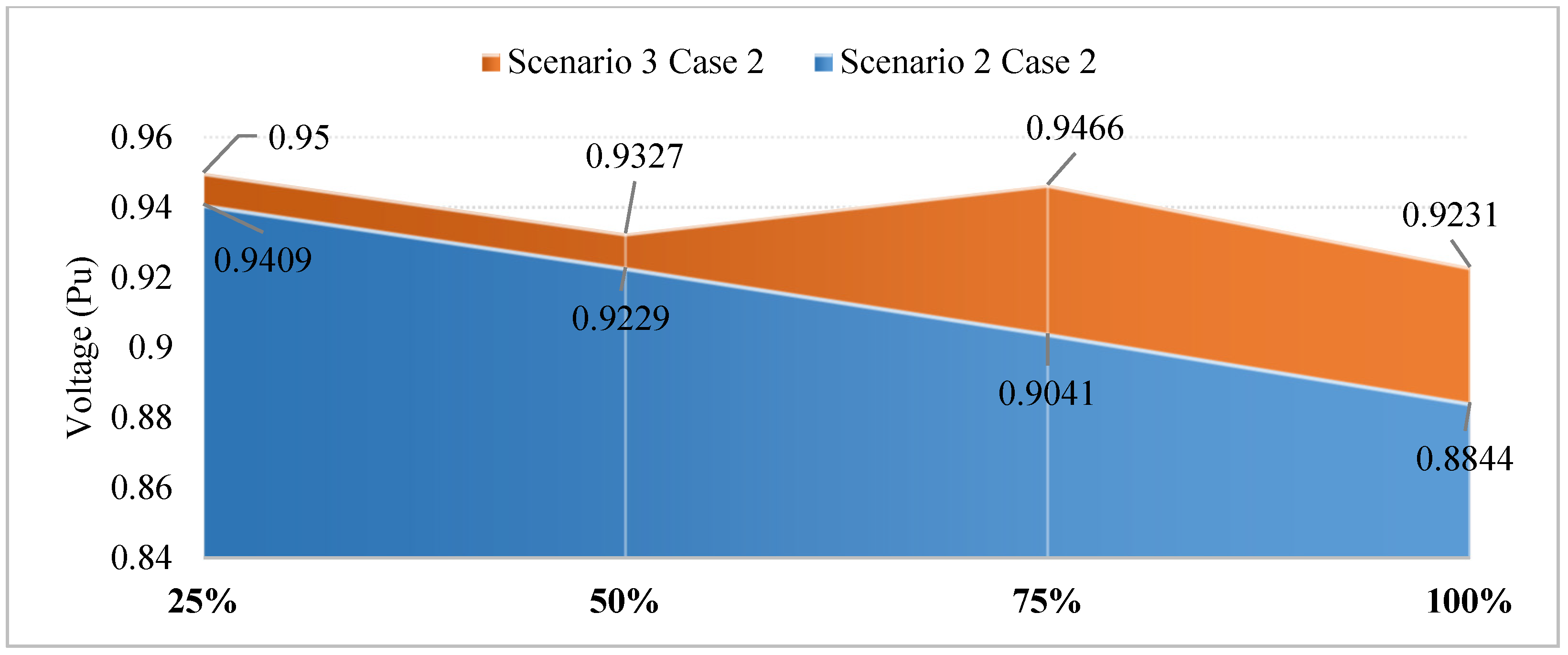
4.2.2. The Results Obtained in Case 2
4.3. The Results Obtained in the Third Scenario
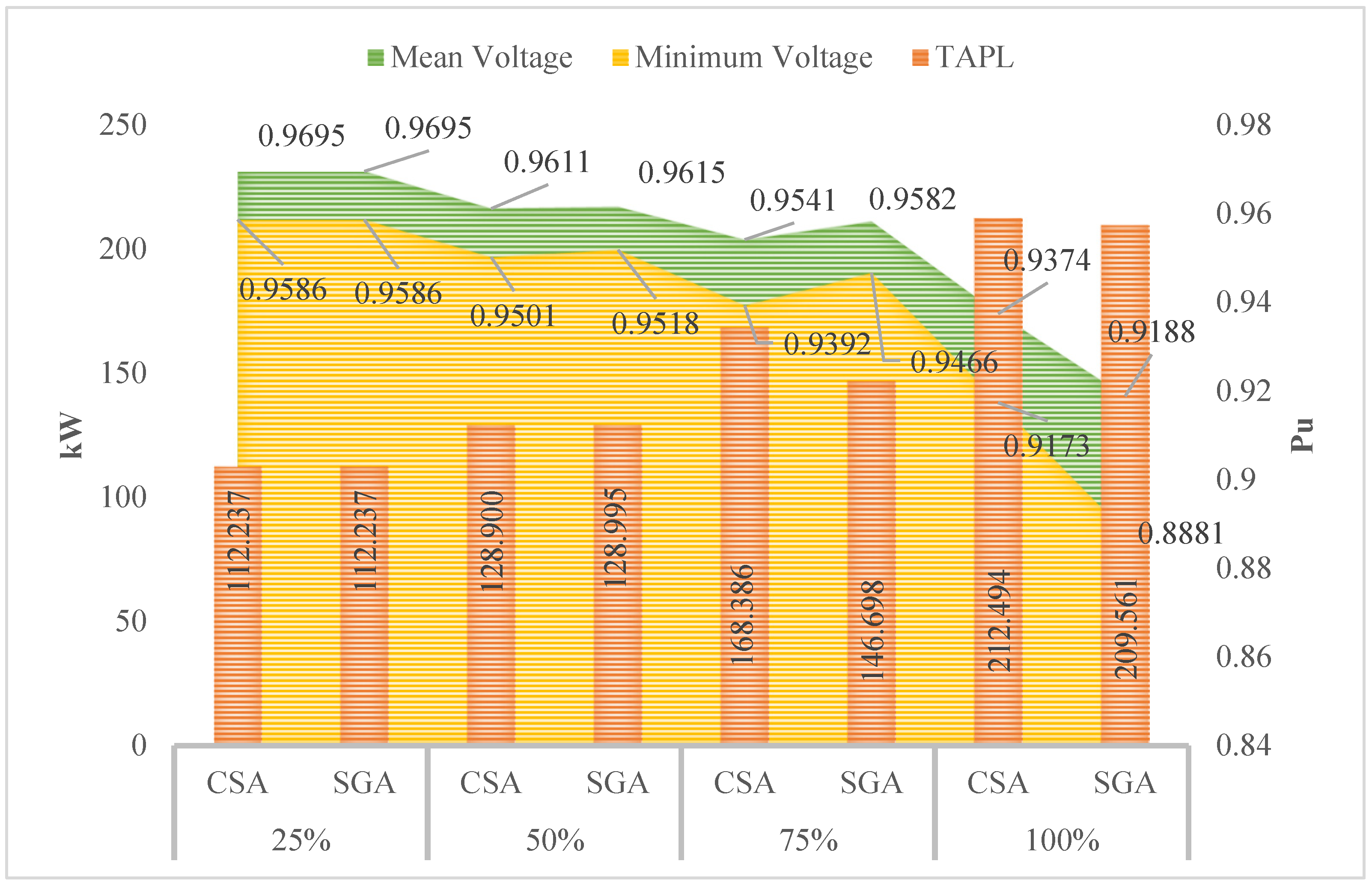
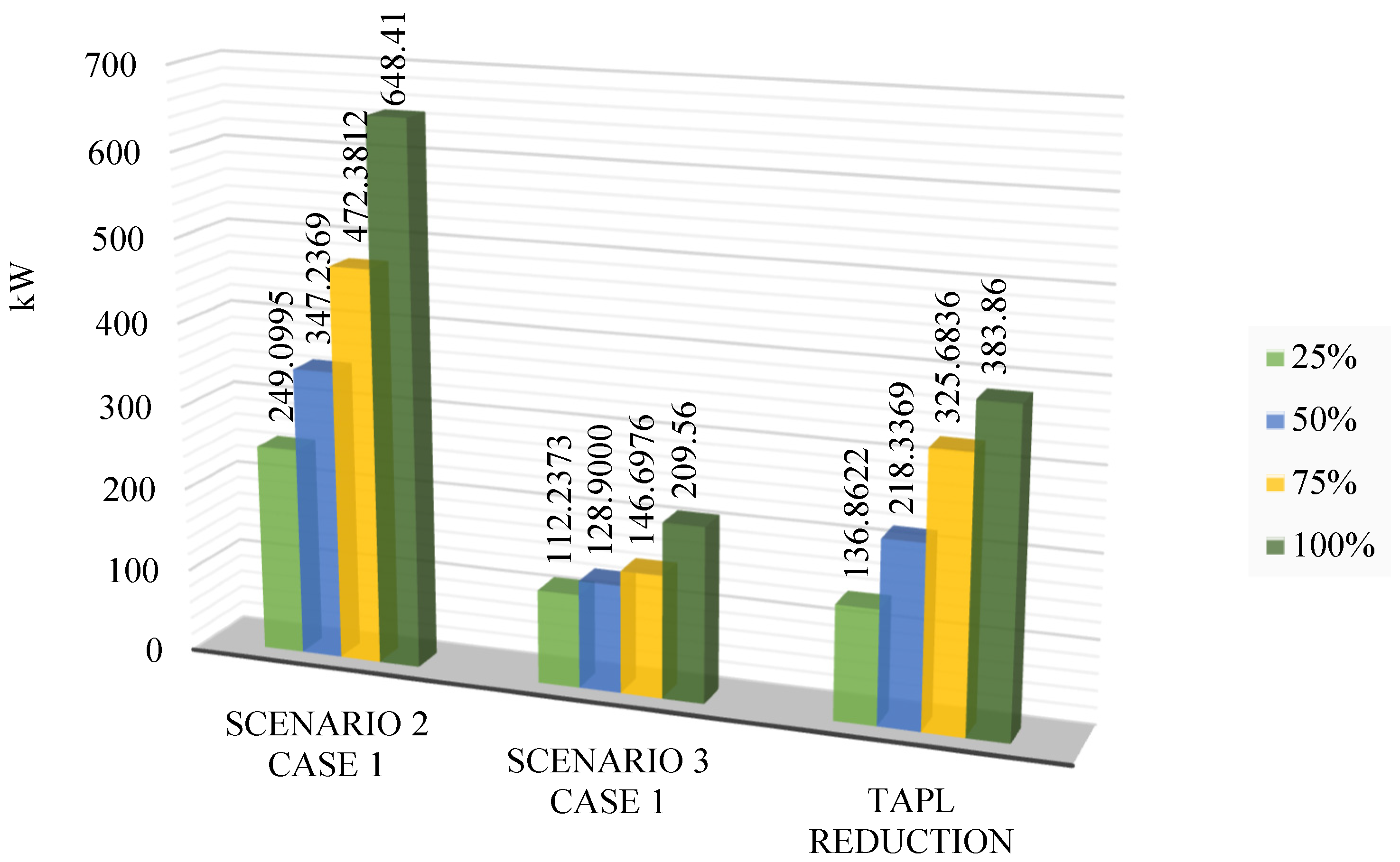
4.3.1. The Results Obtained in Case 1
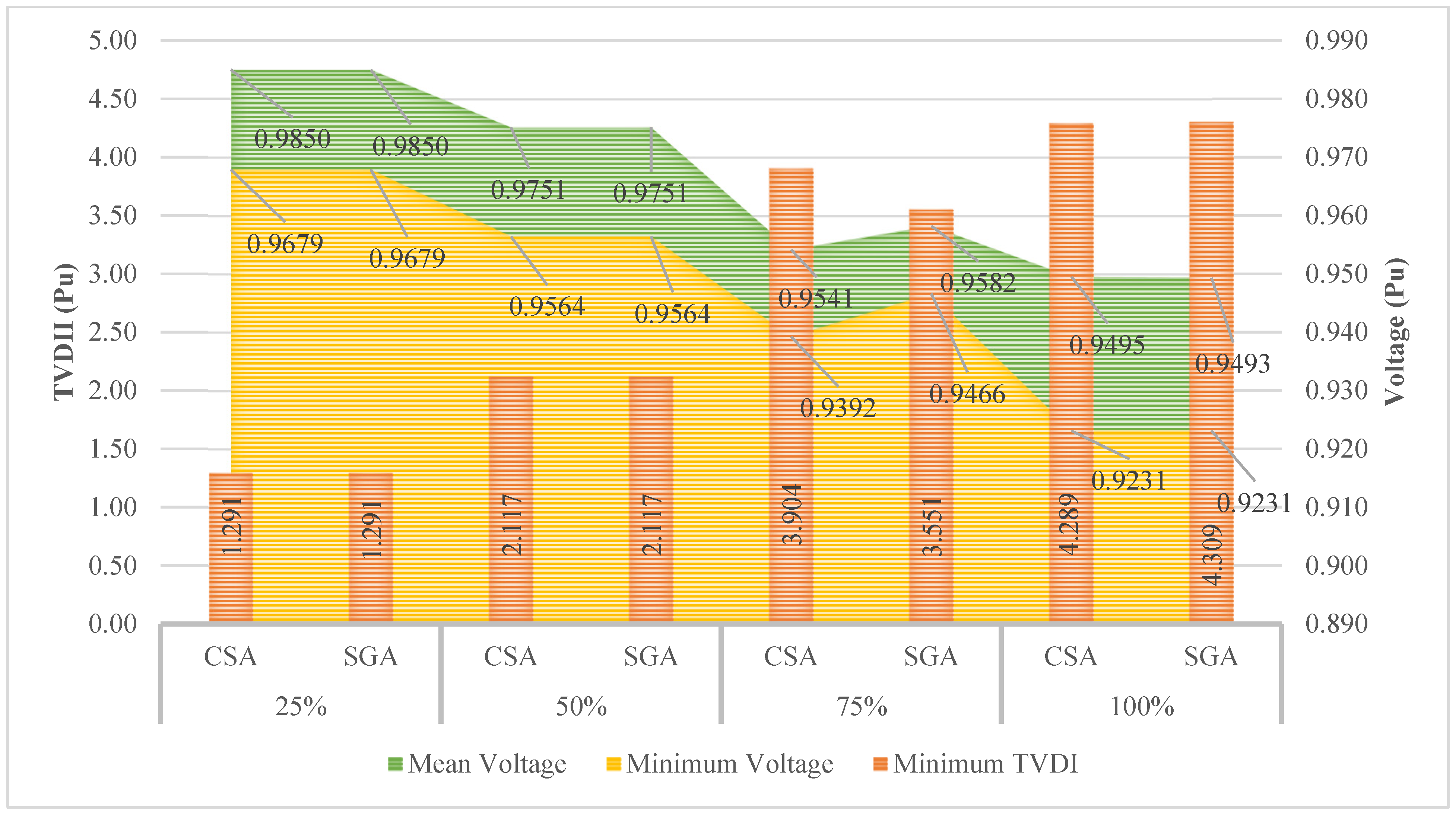
4.3.2. The Results Obtained in Case 2
4.3.3. The Results Obtained in Case 3
4.4. The Results Obtained in the Fourth Scenario
4.4.1. The Results Obtained in Case 1
4.4.2. The Results Obtained in Case 2
4.4.3. The Results Obtained in Case 3
5. Conclusions
- -
- The study only focuses on solving the considered problem in the aspect of planning and expanding the current DEPG, while the operational process is not considered.
- -
- The study only applies the geographical constraints when placing EVCSs, and these constraints are not applied when placing other auxiliary devices.
- -
- The penetration of renewable energy sources such as PVs is not thoroughly evaluated and assessed by using real data.
- -
- SGA is proven to be the better algorithm in two out of three objective functions; however, the method is unstable due to high STD value, especially while dealing with the larger scale of the considered problem with a high penetration level of EVCSs and a large number of desired control variables.
Author Contributions
Funding
Institutional Review Board Statement
Informed Consent Statement
Data Availability Statement
Conflicts of Interest
Nomenclature
| The active power of load at node n | |
| , | Number of installed level 1, level 2 and level 3 EVCSs |
| , and | Active power demand of each Level-1, Level-2 and Level-3 EVCS |
| Reactive power supplied by the grid | |
| Number of all installed capacitor banks | |
| Capacity of the cth installed capacitor bank | |
| Reactive power deamand of the load at node n | |
| Reactance of the dlth distribution line | |
| , | The minimum and maximum reactive power supplied by the SC c |
| Location of the yth installed PV system | |
| Location of Type-1, Type-2 and Type-3 EVCSs. | |
| Location set of Type-1, Type-2 and Type-3 EVCSs | |
| The newly updated individual n in Stage 1 | |
| NPs | The initial population size |
| The nth current solution | |
| Exploration factors manipulating the exploration capabilities | |
| The so-far best location of the individual n | |
| The best location of the whole population | |
| , , | Random factors between zero and one |
| Reference coefficient determining the method of updating a particular individual | |
| , , | The parameters that used to manipulate the exploitation capabilities |
| The current and the highest indexes of the iteration | |
| Upper and lower location bounds for all individuals | |
| Random values between zero and one | |
| , | The current and new velocities of the nth individual |
| The new location updated in Stage 2 for the individual n | |
| , | The influence factors |
| , | Random factor between zero and one |
| , , | Adaptive factors |
| Regulation term | |
| Fitness value of the individual n | |
| The worst individual evaluated by its fitness function | |
| The random factor and its value is between zero and one | |
| The value determined by the Brownian distribution |
Appendix A

| Penetration Level | 25% | 50% | 75% | 100% | ||||
|---|---|---|---|---|---|---|---|---|
| Method | CSA | SGA | CSA | SGA | CSA | SGA | CSA | SGA |
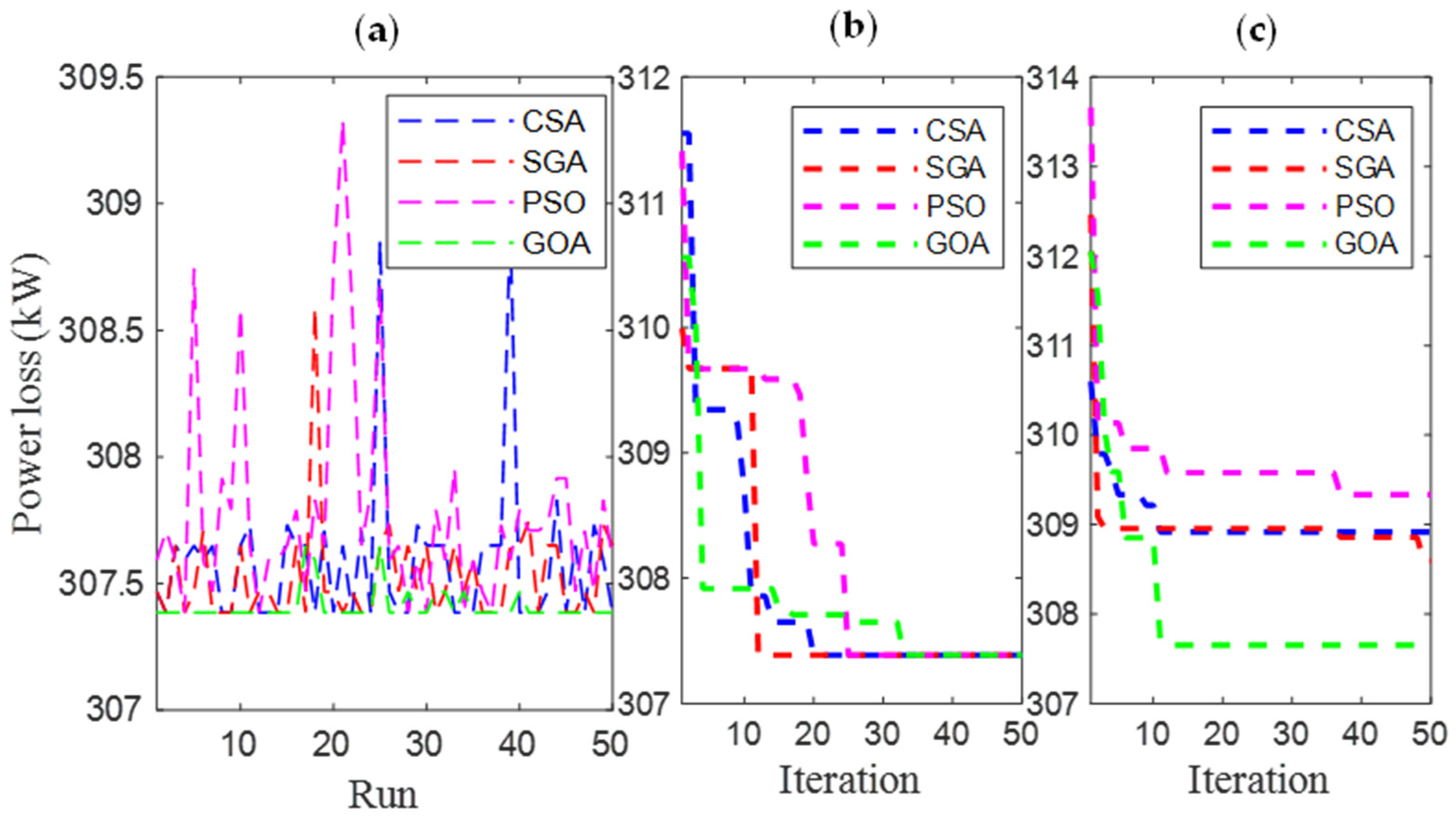
| Minimum Power loss (kW) | 307.3848461 | 307.3848461 | 419.0020249 | 419.0020249 | 562.9795245 | 562.9795245 | 744.053316 | 744.053316 |
| (node) | 33 | 33 | 33 | 33 | 33 | 33 | 33 | 33 |
| (node) | 9 | 9 | 9 | 9 | 9 | 9 | 9 | 9 |
| (node) | 65 | 65 | 65 | 65 | 65 | 65 | 65 | 65 |
| Penetration Level | 25% | 50% | 75% | 100% | ||||
|---|---|---|---|---|---|---|---|---|
| Method | CSA | SGA | CSA | SGA | CSA | SGA | CSA | SGA |
| Minimum Power loss (kW) | 251.0882 | 249.0995 | 347.2369 | 347.2369 | 472.3812 | 472.3812 | 648.4134 | 648.4134 |
| (node) | 34 | 34 | 34 | 34 | 34 | 34 | 34 | 34 |
| (node) | 10 | 10 | 10 | 10 | 10 | 10 | 10 | 10 |
| (node) | 66 | 66 | 66 | 66 | 66 | 66 | 66 | 66 |
(node) | 70 | 44 | 69 | 34 | 48 | 34 | 52 | 52 |
(node) | 44 | 52 | 52 | 52 | 69 | 69 | 70 | 44 |
(node) | 52 | 69 | 34 | 69 | 34 | 48 | 44 | 70 |
(kVar) | 840 | 900 | 840 | 900 | 900 | 900 | 870 | 870 |
(kVar) | 900 | 900 | 900 | 900 | 840 | 840 | 900 | 870 |
(kVar) | 900 | 840 | 900 | 840 | 900 | 900 | 870 | 900 |
| Penetration Level | 25% | 50% | 75% | 100% | ||||
|---|---|---|---|---|---|---|---|---|
| Method | CSA | SGA | CSA | SGA | CSA | SGA | CSA | SGA |
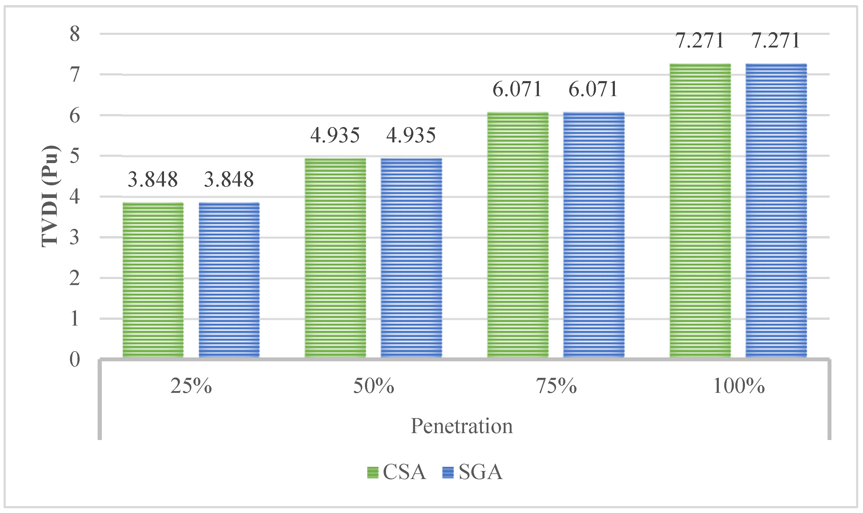
| Minimum TVDI (Pu) | 3.8481 | 3.8481 | 4.9349 | 4.9349 | 6.0713 | 6.0713 | 7.2707 | 7.2707 |
| (node) | 33 | 33 | 33 | 33 | 33 | 33 | 33 | 33 |
| (node) | 9 | 9 | 9 | 9 | 9 | 9 | 9 | 9 |
| (node) | 65 | 65 | 65 | 65 | 65 | 65 | 65 | 65 |
(node) | 68 | 68 | 51 | 33 | 47 | 68 | 69 | 43 |
(node) | 51 | 51 | 33 | 51 | 33 | 47 | 51 | 51 |
(node) | 43 | 43 | 68 | 68 | 68 | 33 | 43 | 69 |
(kVar) | 840 | 840 | 900 | 900 | 900 | 840 | 900 | 900 |
(kVar) | 900 | 900 | 900 | 900 | 900 | 900 | 870 | 840 |
(kVar) | 900 | 900 | 840 | 840 | 840 | 900 | 870 | 900 |
| Penetration Level | 25% | 50% | 75% | 100% | ||||
|---|---|---|---|---|---|---|---|---|
| Method | CSA | SGA | CSA | SGA | CSA | SGA | CSA | SGA |
| Minimum Power loss (kW) | 112.2373 | 112.2373 | 128.9000 | 128.9948 | 168.3862 | 146.6976 | 264.5539 | 332.2845 |
| (node) | 33 | 33 | 33 | 33 | 33 | 33 | 33 | 33 |
| (node) | 9 | 9 | 9 | 9 | 9 | 9 | 9 | 9 |
| (node) | 65 | 65 | 65 | 65 | 65 | 65 | 65 | 65 |
(node) | 33 | 33 | 33 | 64 | 51 | 64 | 44 | 43 |
(node) | 8 | 63 | 57 | 33 | 67 | 47 | 69 | 48 |
| (node) | 63 | 8 | 64 | 57 | 64 | 62 | 48 | 70 |
(kW) | 750 | 750 | 930 | 920 | 900 | 1000 | 620 | 895 |
(kW) | 990 | 870 | 775 | 1000 | 900 | 1000 | 950 | 810 |
(kW) | 870 | 990 | 915 | 700 | 900 | 1000 | 1000 | 945 |
| Penetration Level | 25% | 50% | 75% | 100% | ||||
|---|---|---|---|---|---|---|---|---|
| Method | CSA | SGA | CSA | SGA | CSA | SGA | CSA | SGA |
| Minimum TVDI (Pu) | 1.2908 | 1.2908 | 2.1171 | 2.1171 | 3.9041 | 3.5515 | 4.2890 | 4.3085 |
| (node) | 33 | 33 | 33 | 33 | 33 | 33 | 33 | 33 |
| (node) | 9 | 9 | 9 | 9 | 9 | 9 | 9 | 9 |
| (node) | 65 | 65 | 65 | 65 | 65 | 65 | 65 | 65 |
| (node) | 47 | 40 | 44 | 51 | 51 | 64 | 33 | 69 |
| (node) | 40 | 47 | 51 | 44 | 67 | 62 | 31 | 34 |
| (node) | 69 | 69 | 69 | 69 | 64 | 47 | 69 | 29 |
(kW) | 1000 | 1000 | 1000 | 1000 | 900 | 1000 | 1000 | 1000 |
(kW) | 1000 | 1000 | 1000 | 1000 | 900 | 1000 | 1000 | 1000 |
(kW) | 1000 | 1000 | 1000 | 1000 | 900 | 1000 | 1000 | 1000 |
| Method | CSA | SGA | CSA | SGA | CSA | SGA | CSA | SGA |
|---|---|---|---|---|---|---|---|---|
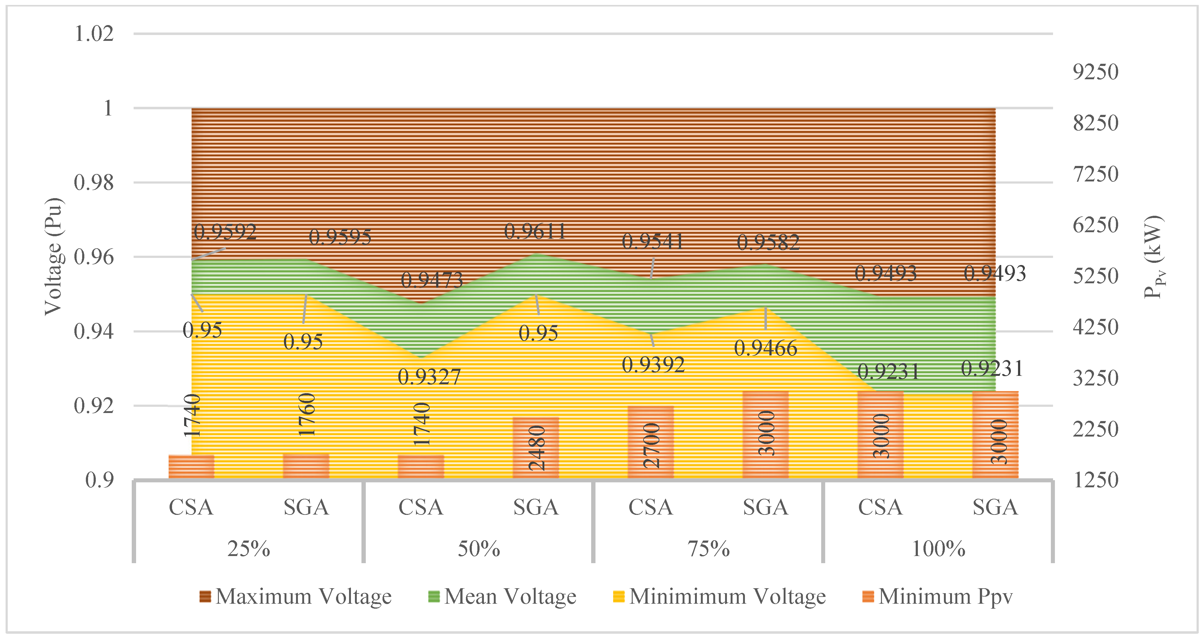
| Minimum PPV (kW) | 1740 | 1760 | 1740 | 2480 | 2700 | 3000 | 3000 | 3000 |
| (node) | 33 | 33 | 33 | 33 | 33 | 33 | 33 | 33 |
| (node) | 9 | 9 | 9 | 9 | 9 | 9 | 9 | 9 |
| (node) | 65 | 65 | 65 | 65 | 65 | 65 | 65 | 65 |
(node) | 50 | 47 | 47 | 67 | 51 | 47 | 29 | 34 |
(node) | 67 | 84 | 67 | 84 | 64 | 62 | 69 | 29 |
(node) | 83 | 69 | 77 | 48 | 67 | 64 | 34 | 69 |
(kW) | 885 | 855 | 940 | 1000 | 900 | 1000 | 1000 | 1000 |
(kW) | 755 | 170 | 995 | 480 | 900 | 1000 | 1000 | 1000 |
(kW) | 100 | 735 | 545 | 1000 | 900 | 1000 | 1000 | 1000 |
| Penetration | 25% | 50% | 75% | 100% | ||||
|---|---|---|---|---|---|---|---|---|
| Method | CSA | SGA | CSA | SGA | CSA | SGA | CSA | SGA |
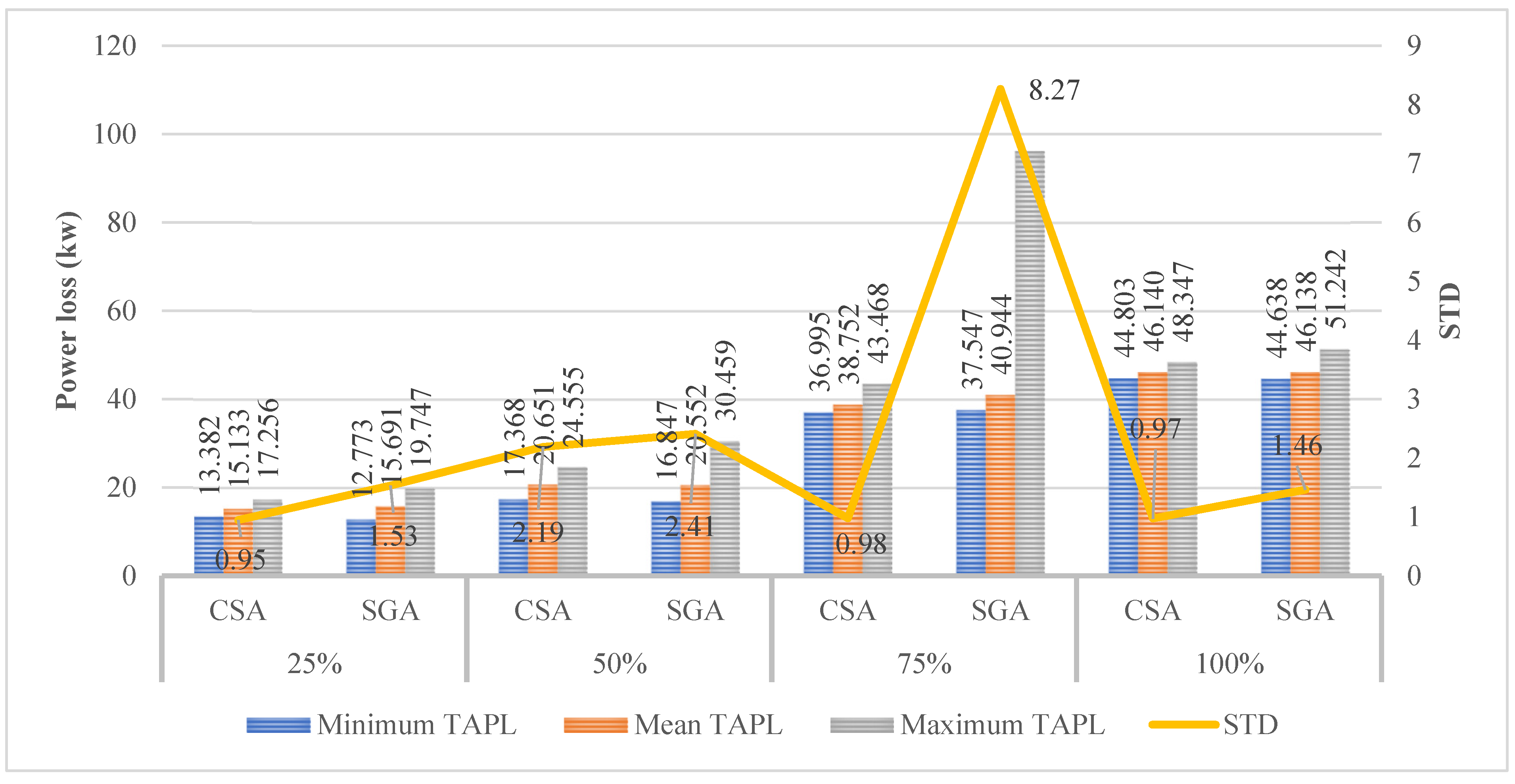
| Minimum TAPL | 13.3818 | 12.7733 | 17.3678 | 16.8469 | 36.9955 | 37.0223 | 44.8032 | 44.6377 |
| (node) | 33 | 33 | 33 | 33 | 33 | 33 | 33 | 33 |
| (node) | 9 | 9 | 9 | 9 | 9 | 9 | 9 | 9 |
| (node) | 65 | 65 | 65 | 65 | 65 | 65 | 65 | 65 |
(node) | 33 | 33 | 8 | 8 | 33 | 24 | 63 | 33 |
(node) | 10 | 66 | 33 | 66 | 10 | 33 | 11 | 66 |
(node) | 63 | 9 | 66 | 34 | 63 | 66 | 32 | 8 |
(kVar) | 750 | 750 | 840 | 900 | 750 | 840 | 750 | 720 |
(kVar) | 630 | 630 | 690 | 630 | 630 | 630 | 480 | 570 |
(kVar) | 690 | 720 | 630 | 600 | 690 | 630 | 870 | 900 |
| (node) | 32 | 63 | 32 | 64 | 57 | 64 | 32 | 32 |
| (node) | 8 | 32 | 56 | 32 | 32 | 57 | 64 | 63 |
| (node) | 66 | 8 | 64 | 8 | 64 | 32 | 63 | 64 |
(kW) | 895 | 900 | 1000 | 1000 | 1000 | 1000 | 1000 | 1000 |
(kW) | 1000 | 870 | 1000 | 1000 | 1000 | 1000 | 1000 | 1000 |
(kW) | 840 | 1000 | 1000 | 1000 | 1000 | 1000 | 1000 | 1000 |
| Penetration | 25% | 50% | 75% | 100% | ||||
|---|---|---|---|---|---|---|---|---|
| Method | CSA | SGA | CSA | SGA | CSA | SGA | CSA | SGA |
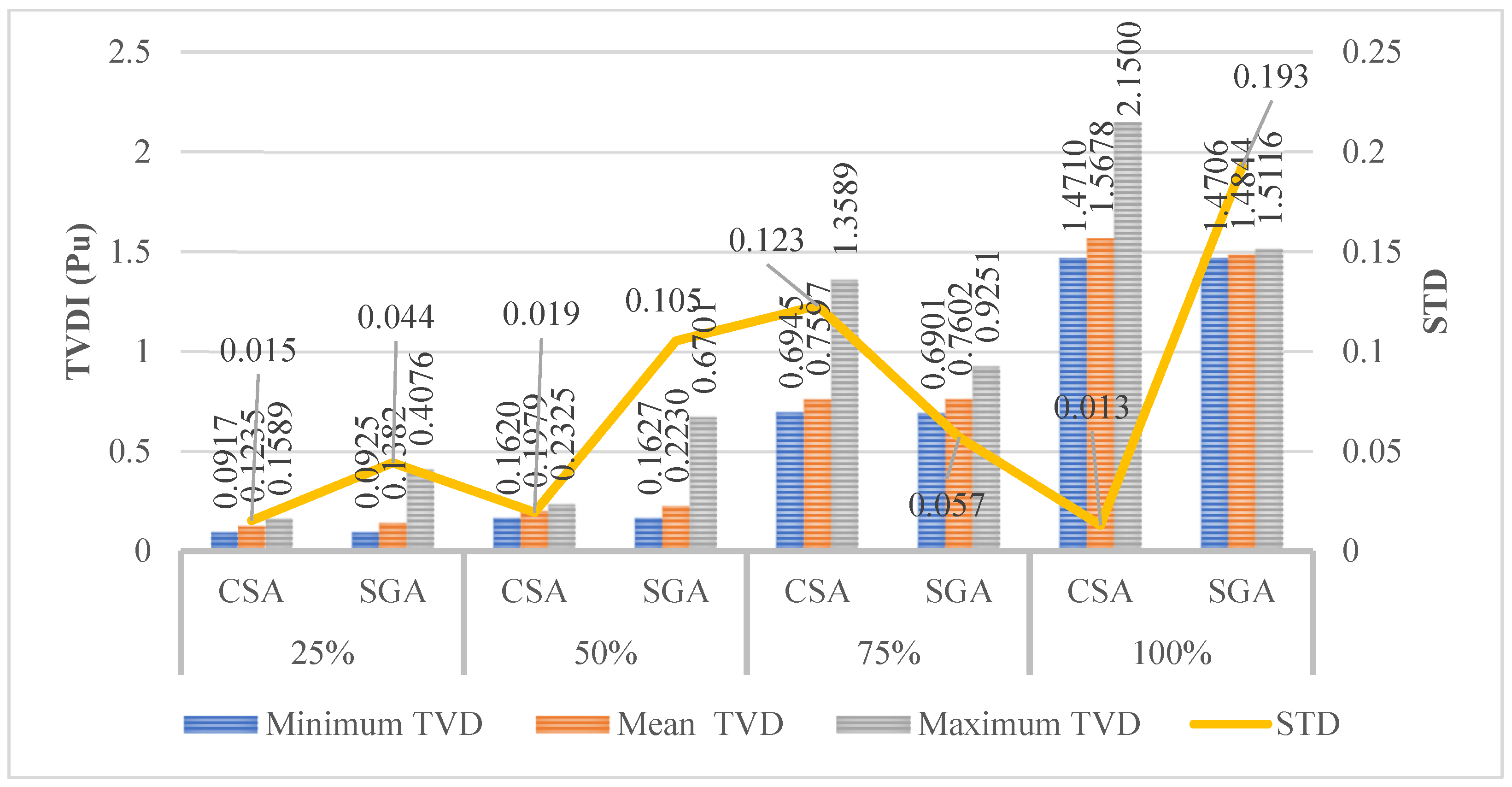
| Minimum TVDII (Pu) | 0.0917 | 0.0925 | 0.1620 | 0.1627 | 0.6945 | 0.6901 | 1.4710 | 1.4706 |
| (node) | 33 | 33 | 33 | 33 | 33 | 33 | 33 | 33 |
| (node) | 9 | 9 | 9 | 9 | 9 | 9 | 9 | 9 |
| (node) | 65 | 65 | 65 | 65 | 65 | 65 | 65 | 65 |
(node) | 51 | 4 | 26 | 30 | 47 | 66 | 68 | 43 |
(node) | 24 | 38 | 47 | 60 | 40 | 40 | 43 | 80 |
(node) | 79 | 57 | 82 | 68 | 71 | 44 | 81 | 68 |
(kVar) | 690 | 900 | 900 | 900 | 900 | 840 | 900 | 900 |
(kVar) | 720 | 810 | 840 | 840 | 900 | 900 | 900 | 840 |
(kVar) | 810 | 900 | 900 | 900 | 840 | 900 | 840 | 900 |
(node) | 56 | 71 | 62 | 64 | 67 | 67 | 47 | 40 |
(node) | 32 | 33 | 32 | 11 | 34 | 47 | 40 | 47 |
(node) | 66 | 10 | 66 | 34 | 65 | 76 | 69 | 69 |
(kW) | 955 | 990 | 1000 | 1000 | 1000 | 1000 | 1000 | 1000 |
(kW) | 885 | 995 | 1000 | 1000 | 1000 | 1000 | 1000 | 1000 |
(kW) | 1000 | 1000 | 1000 | 1000 | 1000 | 1000 | 1000 | 1000 |
| Penetration | 25% | 50% | 75% | 100% | ||||
|---|---|---|---|---|---|---|---|---|
| Method | CSA | SGA | CSA | SGA | CSA | SGA | CSA | SGA |
| Minimum PPV (kW) | 210 | 220 | 775 | 780 | 1385 | 1400 | 2010 | 2020 |
| (node) | 33 | 33 | 33 | 33 | 33 | 33 | 33 | 33 |
| (node) | 9 | 9 | 9 | 9 | 9 | 9 | 9 | 9 |
| (node) | 65 | 65 | 65 | 65 | 65 | 65 | 65 | 65 |
(node) | 43 | 67 | 33 | 33 | 67 | 67 | 65 | 64 |
(node) | 67 | 43 | 65 | 66 | 65 | 76 | 43 | 32 |
(node) | 51 | 47 | 67 | 63 | 51 | 53 | 73 | 84 |
(kVar) | 870 | 900 | 900 | 840 | 900 | 900 | 900 | 900 |
(kVar) | 900 | 840 | 870 | 900 | 870 | 840 | 870 | 900 |
(kVar) | 870 | 900 | 870 | 900 | 870 | 900 | 870 | 840 |
| (node) | 41 | 70 | 35 | 75 | 79 | 84 | 13 | 73 |
| (node) | 64 | 32 | 48 | 52 | 34 | 78 | 49 | 48 |
| (node) | 68 | 33 | 67 | 84 | 71 | 34 | 66 | 76 |
(kW) | 20 | 175 | 545 | 250 | 85 | 105 | 180 | 670 |
(kW) | 35 | 35 | 5 | 530 | 700 | 605 | 855 | 805 |
(kW) | 155 | 10 | 225 | 0 | 600 | 690 | 975 | 545 |
References
- Mariappan, S.; David Raj, A.; Kumar, S.; Chatterjee, U. Global Warming Impacts on the Environment in the Last Century. In Springer Climate; Springer Science and Business Media B.V.: Berlin/Heidelberg, Germany, 2022; pp. 63–93. [Google Scholar]
- Rawat, A.; Kumar, D.; Khati, B.S. A Review on Climate Change Impacts, Models, and Its Consequences on Different Sectors: A Systematic Approach. J. Water Clim. Change 2024, 15, 104–126. [Google Scholar] [CrossRef]
- Yoro, K.O.; Daramola, M.O.; Daramola, M.O. CO2 Emission Sources, Greenhouse Gases, and the Global Warming Effect. In Advances in Carbon Capture; Woodhead Publishing: Saskatoon, UK, 2020; pp. 3–28. [Google Scholar] [CrossRef]
- Delbeke, J.; Runge-Metzger, A.; Slingenberg, Y.; Werksman, J. The Paris Agreement. In Towards a Climate-Neutral Europe; Routledge: Oxfordshire, UK, 2019; pp. 24–45. [Google Scholar]
- Riesz, J.; Sotiriadis, C.; Ambach, D.; Donovan, S. Quantifying the Costs of a Rapid Transition to Electric Vehicles. Appl. Energy 2016, 180, 287–300. [Google Scholar] [CrossRef]
- Chen, Y.; Chen, Y.; Lu, Y. Spatial Accessibility of Public Electric Vehicle Charging Services in China. ISPRS Int. J. Geo-Inf. 2023, 12, 478. [Google Scholar] [CrossRef]
- Mohammadi, F.; Saif, M. A Comprehensive Overview of Electric Vehicle Batteries Market. E-Prime-Adv. Electr. Eng. Electron. Energy 2023, 3, 100127. [Google Scholar] [CrossRef]
- Haces-Fernandez, F. Risk Assessment Framework for Electric Vehicle Charging Station Development in the United States as an Ancillary Service. Energies 2023, 16, 8035. [Google Scholar] [CrossRef]
- Sheng, K.; Dibaj, M.; Akrami, M. Analysing the Cost-Effectiveness of Charging Stations for Electric Vehicles in the U.K.’s Rural Areas. World Electr. Veh. J. 2021, 12, 232. [Google Scholar] [CrossRef]
- Liu, G.; Kang, L.; Luan, Z.; Qiu, J.; Zheng, F. Charging Station and Power Network Planning for Integrated Electric Vehicles (EVs). Energies 2019, 12, 2595. [Google Scholar] [CrossRef]
- Bilal, M.; Rizwan, M. Integration of Electric Vehicle Charging Stations and Capacitors in Distribution Systems with Vehicle-to-Grid Facility. Energy Sources Part A Recovery Util. Environ. Eff. 2021, 1–30. [Google Scholar] [CrossRef]
- Geetha, B.T.; Prakash, A.; Jeyasudha, S.; Dinakaran, K.P. Hybrid Approach Based Combined Allocation of Electric Vehicle Charging Stations and Capacitors in Distribution Systems. J. Energy Storage 2023, 72, 108273. [Google Scholar] [CrossRef]
- Zeb, M.Z.; Imran, K.; Khattak, A.; Janjua, A.K.; Pal, A.; Nadeem, M.; Zhang, J.; Khan, S. Optimal Placement of Electric Vehicle Charging Stations in the Active Distribution Network. IEEE Access 2020, 8, 68124–68134. [Google Scholar] [CrossRef]
- Ahmad, F.; Khalid, M.; Panigrahi, B.K. An Enhanced Approach to Optimally Place the Solar Powered Electric Vehicle Charging Station in Distribution Network. J. Energy Storage 2021, 42, 103090. [Google Scholar] [CrossRef]
- Chen, L.; Xu, C.; Song, H.; Jermsittiparsert, K. Optimal Sizing and Sitting of EVCS in the Distribution System Using Metaheuristics: A Case Study. Energy Rep. 2021, 7, 208–217. [Google Scholar] [CrossRef]
- Balu, K.; Mukherjee, V. Optimal Allocation of Electric Vehicle Charging Stations and Renewable Distributed Generation with Battery Energy Storage in Radial Distribution System Considering Time Sequence Characteristics of Generation and Load Demand. J. Energy Storage 2023, 59, 106533. [Google Scholar] [CrossRef]
- Yuvaraj, T.; Suresh, T.D.; Meyyappan, U.; Aljafari, B.; Thanikanti, S.B. Optimizing the Allocation of Renewable DGs, DSTATCOM, and BESS to Mitigate the Impact of Electric Vehicle Charging Stations on Radial Distribution Systems. Heliyon 2023, 9, e23017. [Google Scholar] [CrossRef]
- Yuvaraj, T.; Devabalaji, K.R.; Thanikanti, S.B.; Pamshetti, V.B.; Nwulu, N.I. Integration of Electric Vehicle Charging Stations and DSTATCOM in Practical Indian Distribution Systems Using Bald Eagle Search Algorithm. IEEE Access 2023, 11, 55149–55168. [Google Scholar] [CrossRef]
- Dharavat, N.; Sudabattula, S.K.; Suresh, V. Optimal Integration of Distributed Generators (DGs) Shunt Capacitors (SCs) and Electric Vehicles (EVs) in a Distribution System (DS) Using Marine Predator Algorithm. Int. J. Renew. Energy Res. 2022, 12, 1637–1650. [Google Scholar] [CrossRef]
- Mohanty, A.K.; Babu, P.S.; Salkuti, S.R. Fuzzy-Based Simultaneous Optimal Placement of Electric Vehicle Charging Stations, Distributed Generators, and DSTATCOM in a Distribution System. Energies 2022, 15, 8702. [Google Scholar] [CrossRef]
- Goli, P.; Jasthi, K.; Gampa, S.R.; Das, D.; Shireen, W.; Siano, P.; Guerrero, J.M. Electric Vehicle Charging Load Allocation at Residential Locations Utilizing the Energy Savings Gained by Optimal Network Reconductoring. Smart Cities 2022, 5, 177–205. [Google Scholar] [CrossRef]
- de Lima, T.D.; Franco, J.F.; Lezama, F.; Soares, J.; Vale, Z. Joint Optimal Allocation of Electric Vehicle Charging Stations and Renewable Energy Sources Including CO2 Emissions. Energy Inform. 2021, 4, 33. [Google Scholar] [CrossRef]
- Liu, L.; Zhang, Y.; Da, C.; Huang, Z.; Wang, M. Optimal Allocation of Distributed Generation and Electric Vehicle Charging Stations Based on Intelligent Algorithm and Bi-level Programming. Int. Trans. Electr. Energy Syst. 2020, 30, e12366. [Google Scholar] [CrossRef]
- Mohammadi, F.; Mirhashemi, M. An Overview of Planning for Vehicle-to-Grid Systems with Large-Scale Adoption of Electric Vehicles. In Proceedings of the 2024 IEEE Global Energy Conference, Riverside, CA, USA; Batman, Türkiye, 4–6 December 2024. [Google Scholar]
- Mohammadi, F.; Mirhashemi, M. An Overview of Ancillary Services Provided by Vehicle-to-Grid Systems. In Proceedings of the 2024 3rd Asia Power and Electrical Technology Conference (APET), Fuzhou, China, 15–17 November 2024. [Google Scholar]
- Kumar, K.J.; Kumar, S.; V.S., N. Standards for Electric Vehicle Charging Stations in India: A Review. Energy Storage 2022, 4, e261. [Google Scholar] [CrossRef]
- Marinescu, C. Progress in the Development and Implementation of Residential EV Charging Stations Based on Renewable Energy Sources. Energies 2022, 16, 179. [Google Scholar] [CrossRef]
- Braik, M.S. Chameleon Swarm Algorithm: A Bio-Inspired Optimizer for Solving Engineering Design Problems. Expert Syst. Appl. 2021, 174, 114685. [Google Scholar] [CrossRef]
- Tian, A.-Q.; Liu, F.-F.; Lv, H.-X. Snow Geese Algorithm: A Novel Migration-Inspired Meta-Heuristic Algorithm for Constrained Engineering Optimization Problems. Appl. Math. Model. 2024, 126, 327–347. [Google Scholar] [CrossRef]
- Bakhtvar, M.; Keane, A. Allocation of Wind Capacity Subject to Long Term Voltage Stability Constraints. IEEE Trans. Power Syst. 2016, 31, 2404–2414. [Google Scholar] [CrossRef]
- Zhu, H.; Liu, H.J. Fast Local Voltage Control Under Limited Reactive Power: Optimality and Stability Analysis. IEEE Trans. Power Syst. 2016, 31, 3794–3803. [Google Scholar] [CrossRef]
- Specifications of Electric Vehicle Charging Station from VinFast Company. Available online: https://vinfast.vn/thu-vien/tram-sac-va-pin/he-thong-tram-sac-vinfast-cap-nhat-moi-nhat/ (accessed on 10 February 2025).
- Phan, T.M.; Duong, M.P.; Doan, A.T.; Duong, M.Q.; Nguyen, T.T. Optimal Design and Operation of Wind Turbines in Radial Distribution Power Grids for Power Loss Minimization. Appl. Sci. 2024, 14, 1462. [Google Scholar] [CrossRef]
- Smith, J.; Doe, A.; Brown, K. Golf Optimization Algorithm: A New Game-Based Metaheuristic Algorithm and Its Application to Energy Commitment Problem Considering Resilience. Energies 2023, 8, 386. [Google Scholar] [CrossRef]
- Kennedy, J.; Eberhart, R. Particle swarm optimization. In Proceedings of the ICNN’95 - International Conference on Neural Networks, Perth, WA, Australia, 27 November–1 December 1995; Volume 4, pp. 1942–1948. [Google Scholar] [CrossRef]


| Scenario | Auxiliary Devices | Case Study | Main Objective Function | Number of Control Variables | Presets (NPs–HI) | |
|---|---|---|---|---|---|---|
| CSA | SGA | |||||
| 1 | None | 1 | Minimizing the total active power loss | 3 | 20–50 | 40–50 |
| 2 | SCs | 1 | Minimizing the total active power loss | 6 | 30–200 | 60–200 |
| 2 | Minimizing total voltage deviation | 6 | 30–200 | 60–200 | ||
| 3 | 03 PVs | 1 | Minimizing the total active power loss | 6 | 30–200 | 60–200 |
| 2 | Minimizing total voltage deviation | 6 | 30–200 | 60–200 | ||
| 3 | Minimizing total PV’s rated power | 6 | 30–200 | 60–200 | ||
| 4 | 3PVs + 3SCs | 1 | Minimizing the total active power loss | 12 | 50–300 | 100–300 |
| 2 | Minimizing total voltage deviation | 12 | 50–300 | 100–300 | ||
| 3 | Minimizing total PV’s rated power | 12 | 50–300 | 100–300 | ||
| Scenario | The Penetration of EVCSs (%) | Number of EVCSs for Each Level |
|---|---|---|
| 1, 2, 3, 4 | 25 | 4LV1–4LV2–2LV3 |
| 50 | 8LV1–8LV2–4LV3 | |
| 75 | 12LV1–12LV2–6LV3 | |
| 100 | 16LV1–16LV2–8LV3 |
Disclaimer/Publisher’s Note: The statements, opinions and data contained in all publications are solely those of the individual author(s) and contributor(s) and not of MDPI and/or the editor(s). MDPI and/or the editor(s) disclaim responsibility for any injury to people or property resulting from any ideas, methods, instructions or products referred to in the content. |
© 2025 by the authors. Licensee MDPI, Basel, Switzerland. This article is an open access article distributed under the terms and conditions of the Creative Commons Attribution (CC BY) license (https://creativecommons.org/licenses/by/4.0/).
Share and Cite
Kien, L.C.; Loi, T.D.; Duong, M.P.; Nguyen, T.T. Energy Loss Reduction for Distribution Electric Power Systems with Renewable Power Sources, Reactive Power Compensators, and Electric Vehicle Charge Stations. Sensors 2025, 25, 1997. https://doi.org/10.3390/s25071997
Kien LC, Loi TD, Duong MP, Nguyen TT. Energy Loss Reduction for Distribution Electric Power Systems with Renewable Power Sources, Reactive Power Compensators, and Electric Vehicle Charge Stations. Sensors. 2025; 25(7):1997. https://doi.org/10.3390/s25071997
Chicago/Turabian StyleKien, Le Chi, Tran Duc Loi, Minh Phuc Duong, and Thang Trung Nguyen. 2025. "Energy Loss Reduction for Distribution Electric Power Systems with Renewable Power Sources, Reactive Power Compensators, and Electric Vehicle Charge Stations" Sensors 25, no. 7: 1997. https://doi.org/10.3390/s25071997
APA StyleKien, L. C., Loi, T. D., Duong, M. P., & Nguyen, T. T. (2025). Energy Loss Reduction for Distribution Electric Power Systems with Renewable Power Sources, Reactive Power Compensators, and Electric Vehicle Charge Stations. Sensors, 25(7), 1997. https://doi.org/10.3390/s25071997