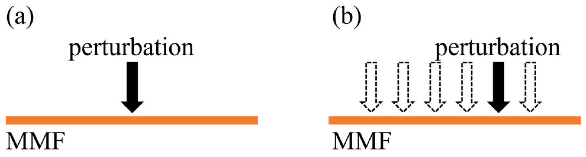
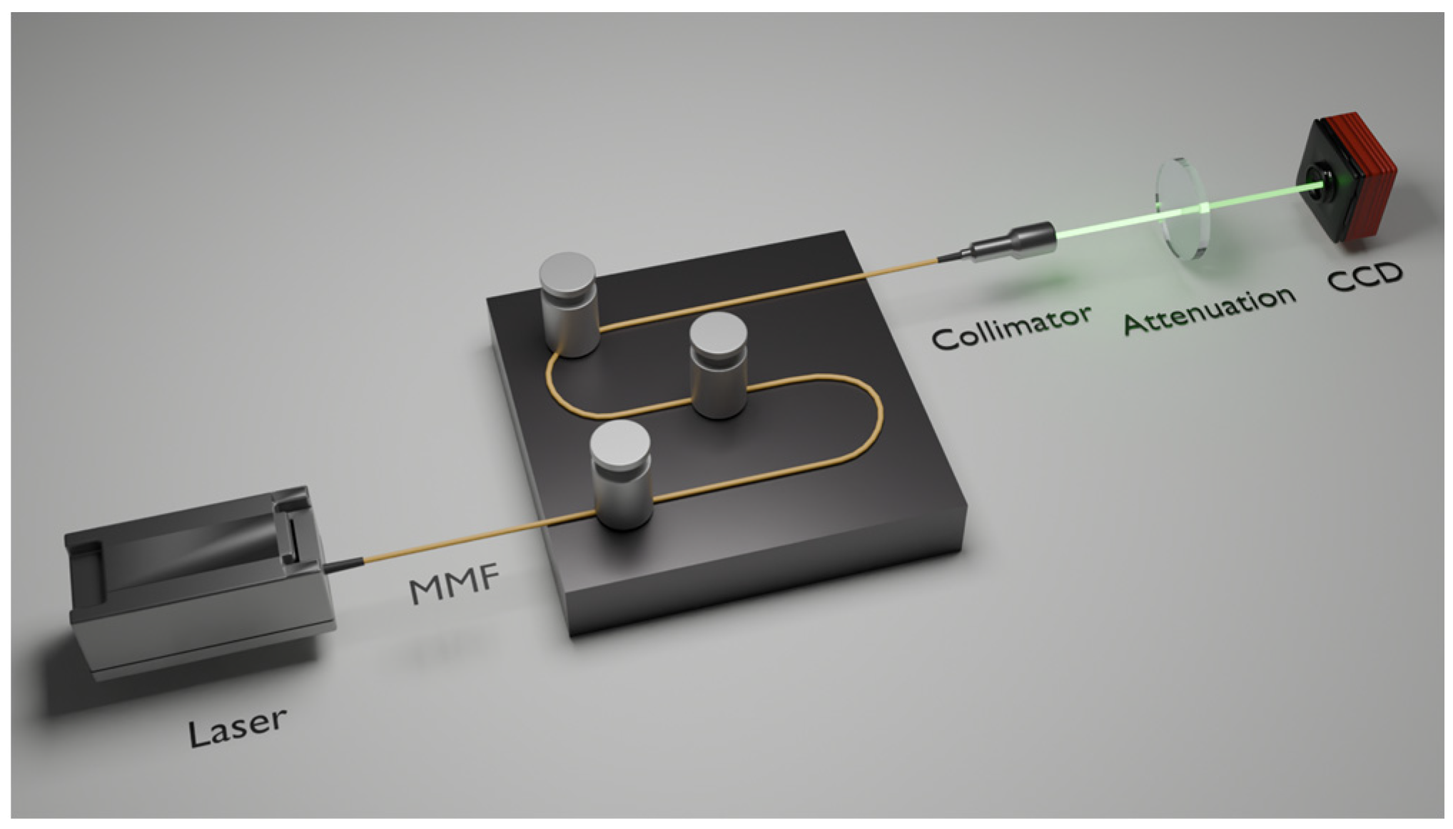
Figure 1.
Schematic diagram of experimental setup for studying specklegram variations in MMF: (a) various perturbation intensities applied at the same position; (b) same perturbation intensity applied on different positions (dotted arrows indicate perturbation locations).
Figure 1.
Schematic diagram of experimental setup for studying specklegram variations in MMF: (a) various perturbation intensities applied at the same position; (b) same perturbation intensity applied on different positions (dotted arrows indicate perturbation locations).
Figure 2.
Schematic diagram of the 3 × 3 division of specklegram images.
Figure 2.
Schematic diagram of the 3 × 3 division of specklegram images.
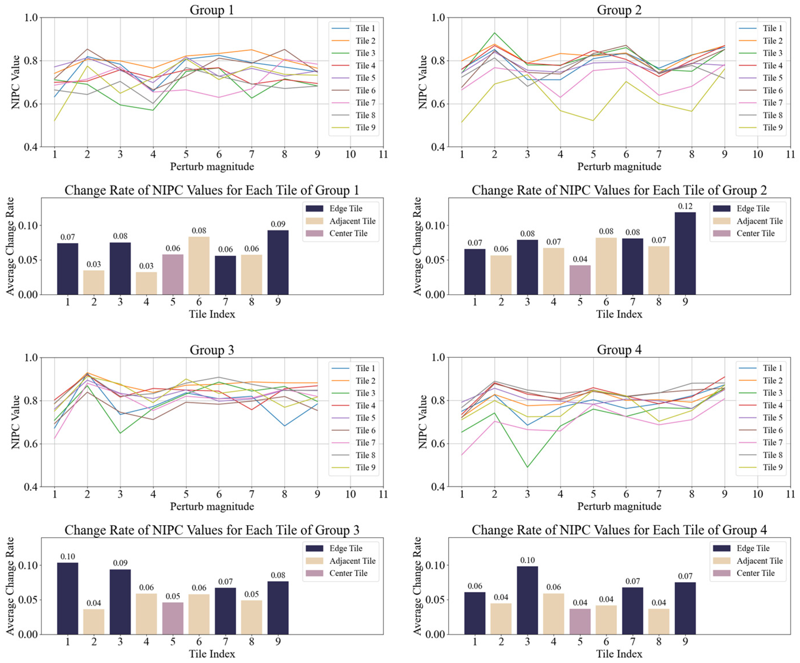
Figure 3.
NIPC and average change rate of each tile under varying perturbation intensities on same position.
Figure 3.
NIPC and average change rate of each tile under varying perturbation intensities on same position.
Figure 4.
NIPC and average change rate of each tile under perturbation at different positions.
Figure 4.
NIPC and average change rate of each tile under perturbation at different positions.
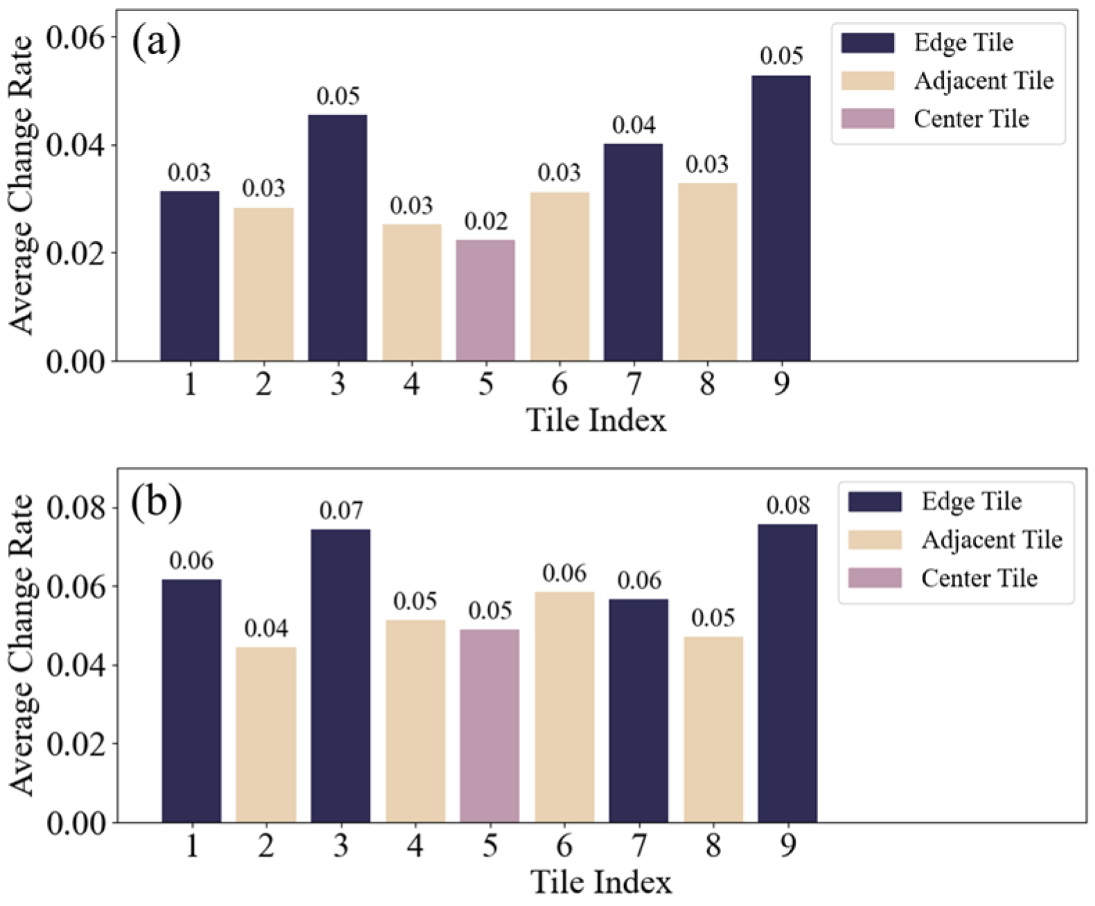
Figure 5.
Average change rate of ten group for each tile: (a) continuous varying perturbation intensities on same position; (b) same perturbation at different positions.
Figure 5.
Average change rate of ten group for each tile: (a) continuous varying perturbation intensities on same position; (b) same perturbation at different positions.
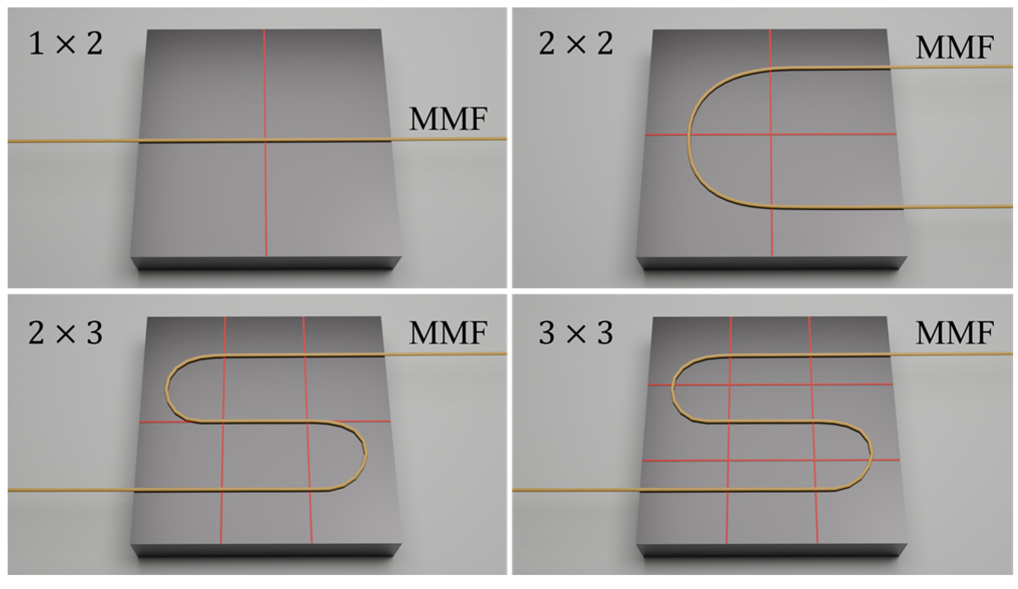
Figure 6.
Diagram of grid divisions and fiber placement.
Figure 6.
Diagram of grid divisions and fiber placement.
Figure 7.
Diagram of loads on MMF (the condition of three loads applied on the 3 × 3 plane).
Figure 7.
Diagram of loads on MMF (the condition of three loads applied on the 3 × 3 plane).
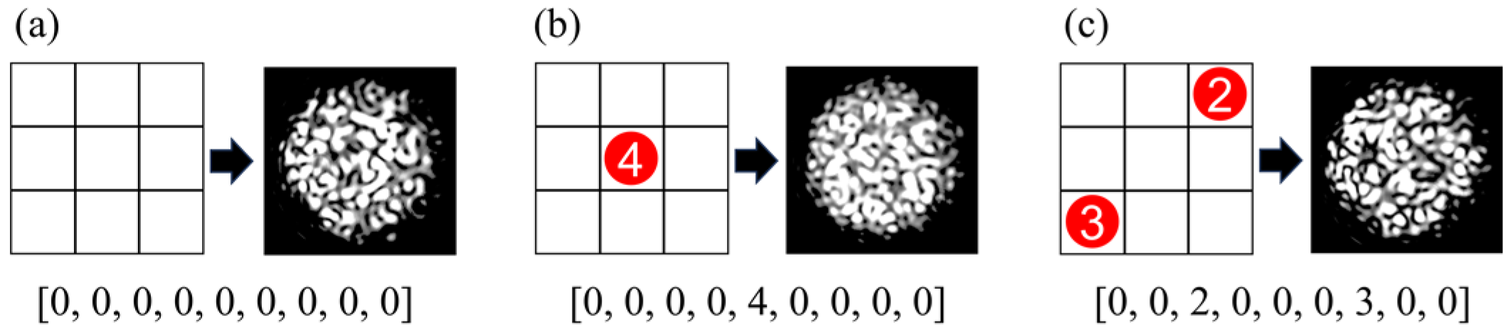
Figure 8.
Diagram of perturbation position and intensity with the corresponding specklegram sample annotation: (a) [0, 0, 0, 0, 0, 0, 0, 0, 0] indicates no weights are applied; (b) [0, 0, 0, 0, 4, 0, 0, 0, 0] indicates four weights are applied in the fifth position on the planar; (c) [0, 0, 2, 0, 0, 0, 3, 0, 0] indicates two and three weights are applied in the third and seventh position on the planar, respectively.
Figure 9.
Generation of specklegram by traversal occlusion.
Figure 9.
Generation of specklegram by traversal occlusion.
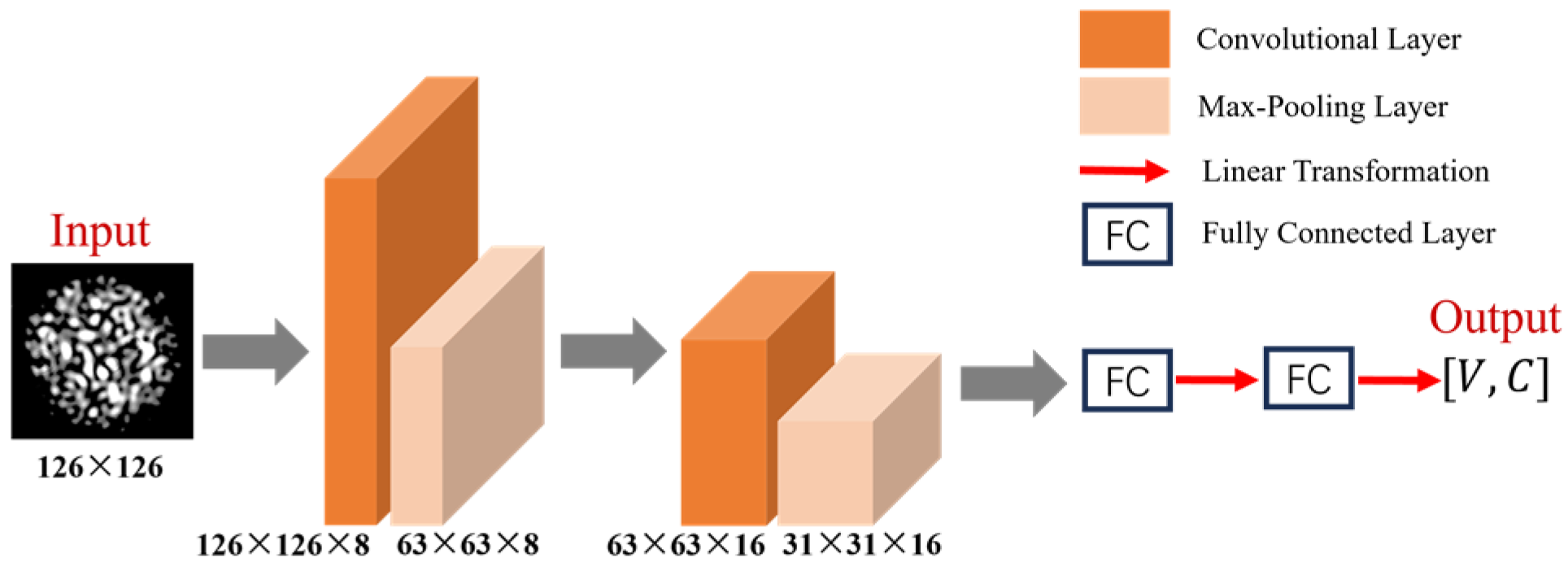
Figure 10.
Architecture of the shallow CNN.
Figure 10.
Architecture of the shallow CNN.
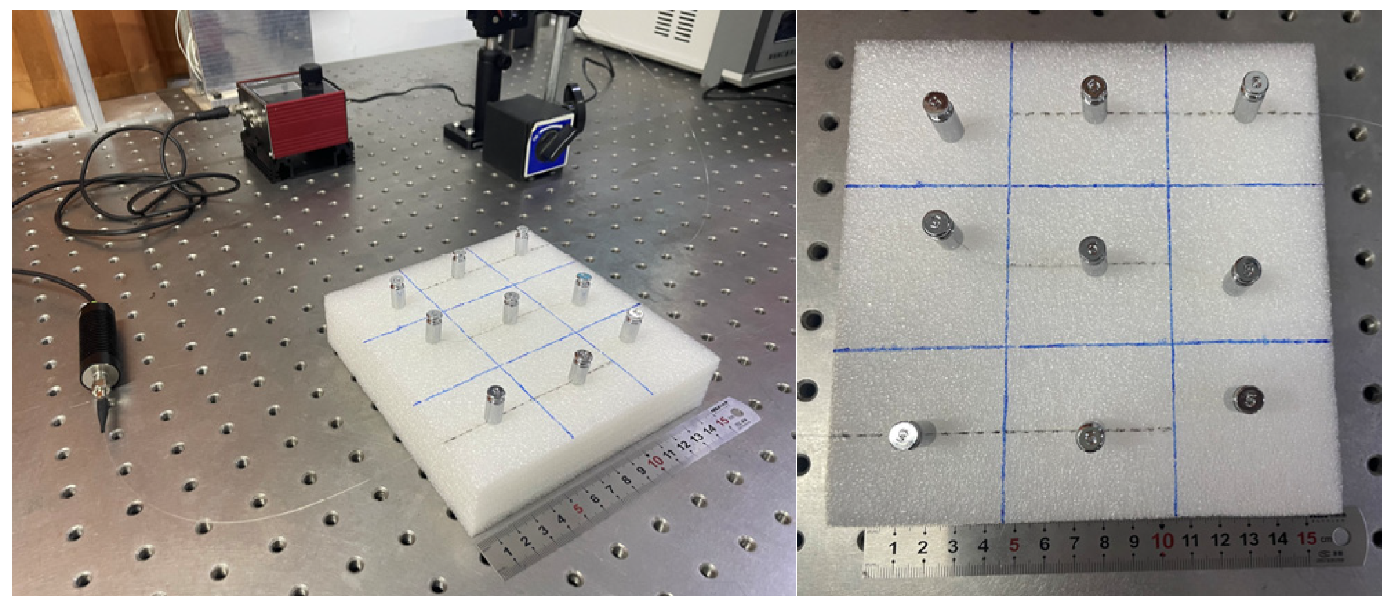
Figure 11.
Diagram of the experimental setup for recognition of the load distribution on the foam.
Figure 11.
Diagram of the experimental setup for recognition of the load distribution on the foam.
Figure 12.
Diagram of the positions of the weight on the foam.
Figure 12.
Diagram of the positions of the weight on the foam.
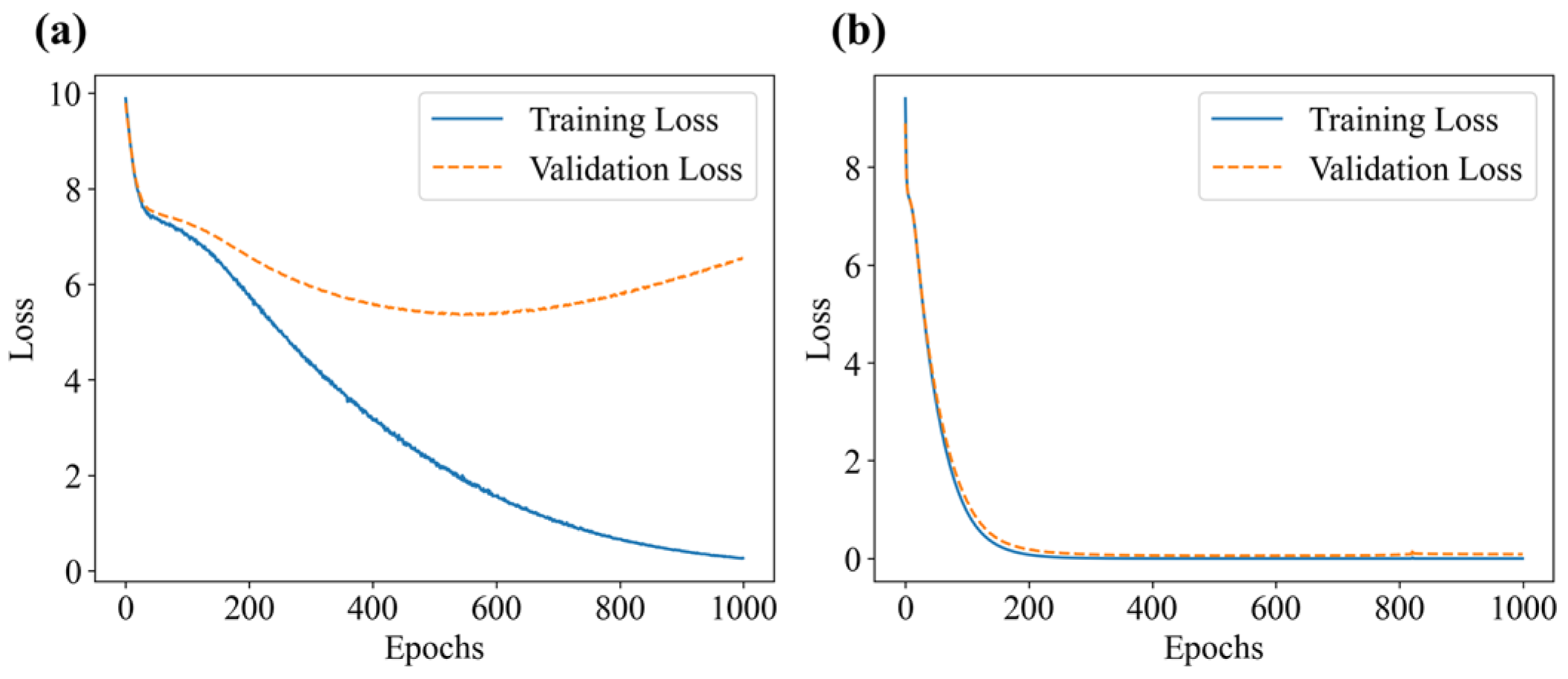
Figure 13.
Loss function plot during the training process: (a) without occlusion; (b) with occlusion.
Figure 13.
Loss function plot during the training process: (a) without occlusion; (b) with occlusion.
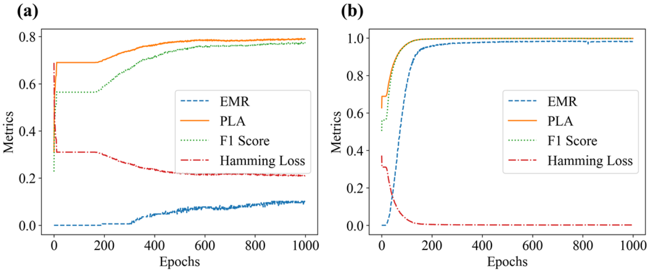
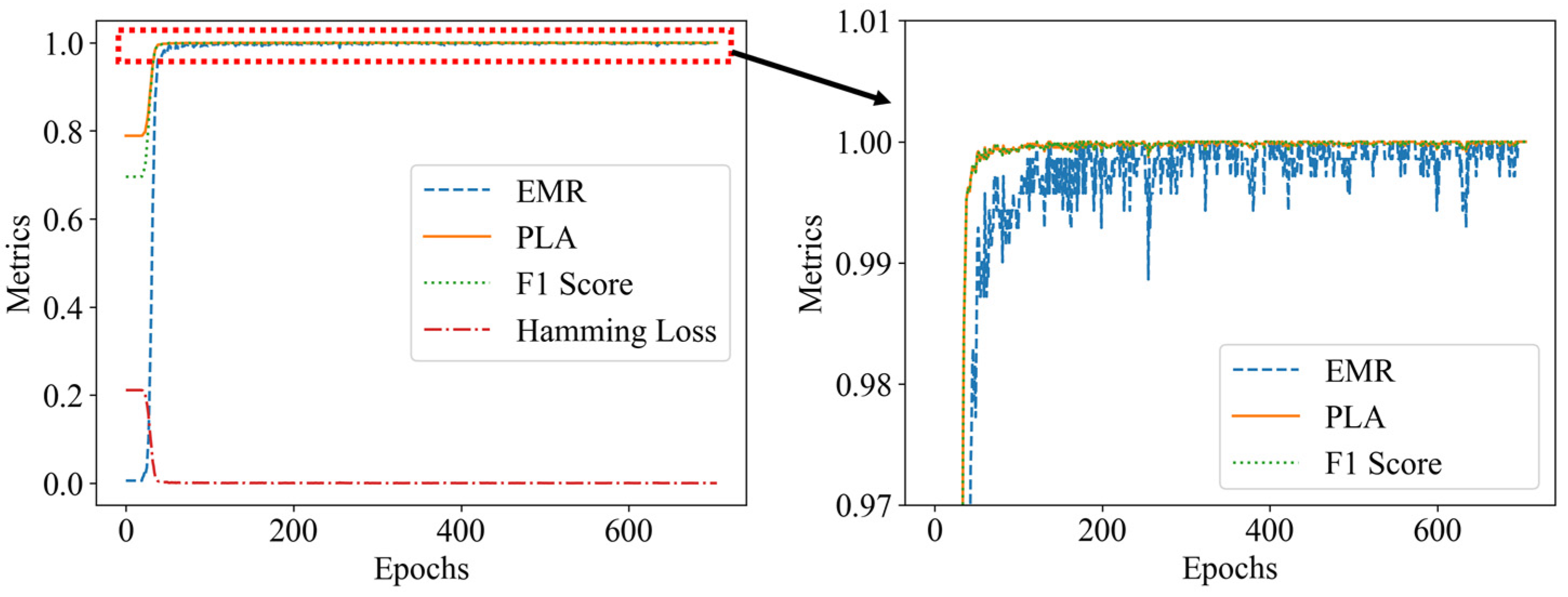
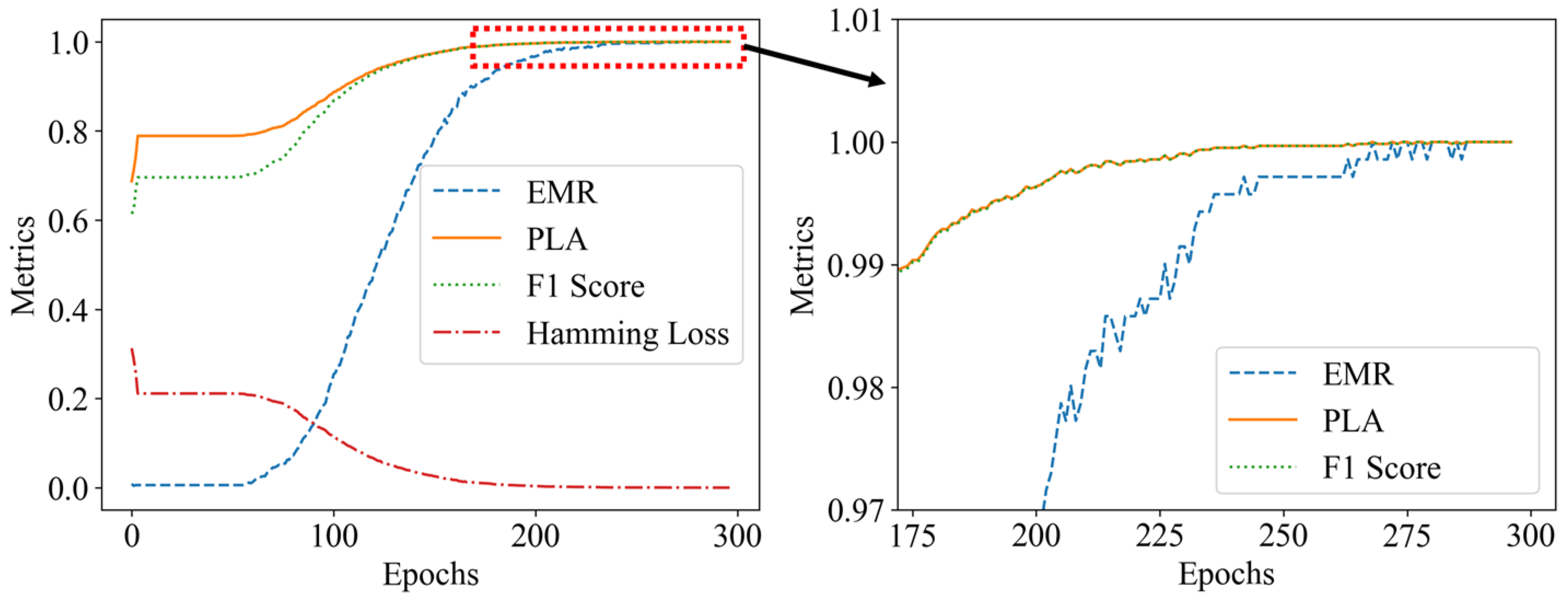
Figure 14.
Model evaluation metrics plot: (a) without occlusion; (b) with occlusion.
Figure 14.
Model evaluation metrics plot: (a) without occlusion; (b) with occlusion.
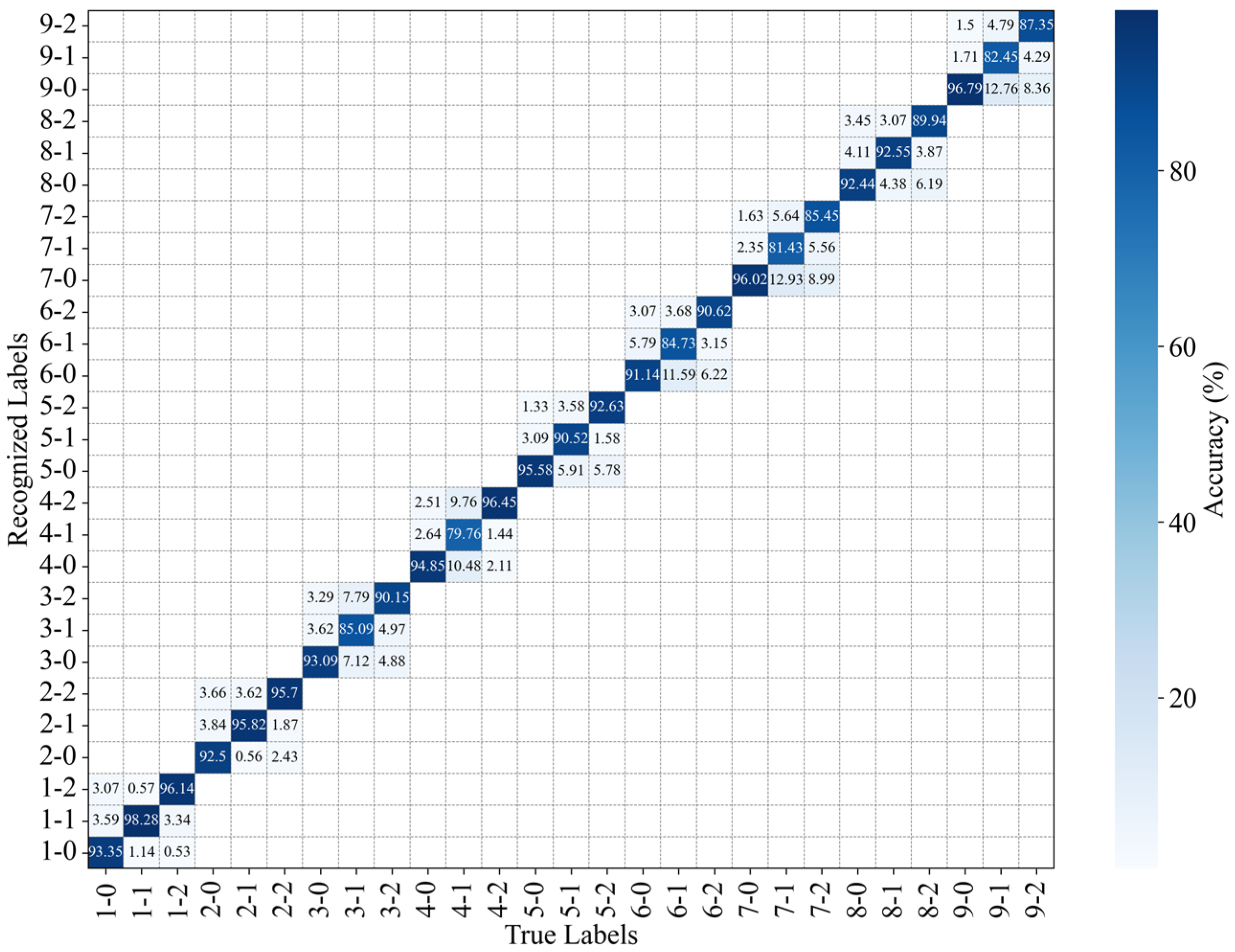
Figure 15.
Recognition accuracy of the position and intensity of perturbations without occlusion.
Figure 15.
Recognition accuracy of the position and intensity of perturbations without occlusion.
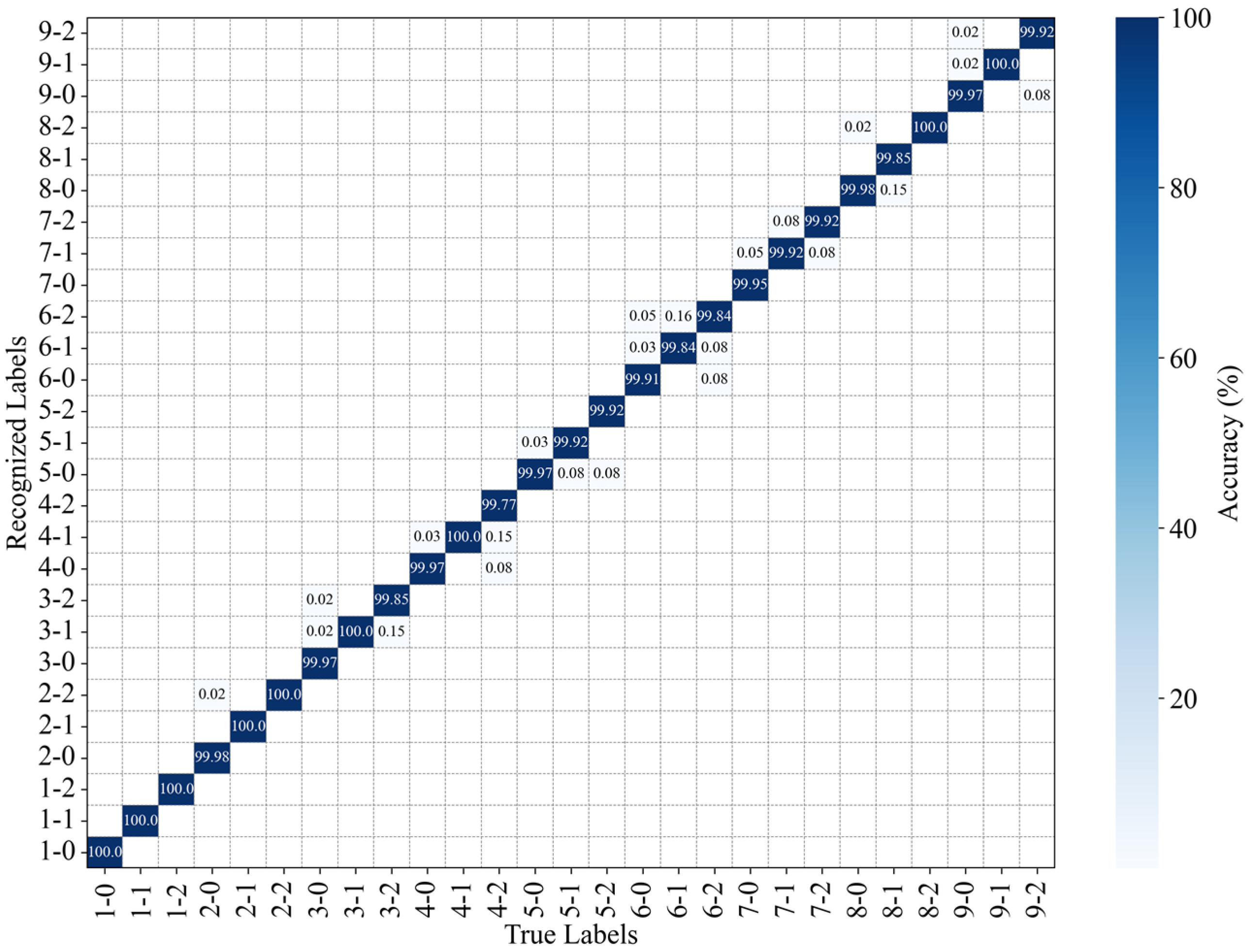
Figure 16.
Recognition accuracy of the position and intensity of perturbations with occlusion.
Figure 16.
Recognition accuracy of the position and intensity of perturbations with occlusion.
Figure 17.
Process of converting input specklegram into load spatial distribution.
Figure 17.
Process of converting input specklegram into load spatial distribution.
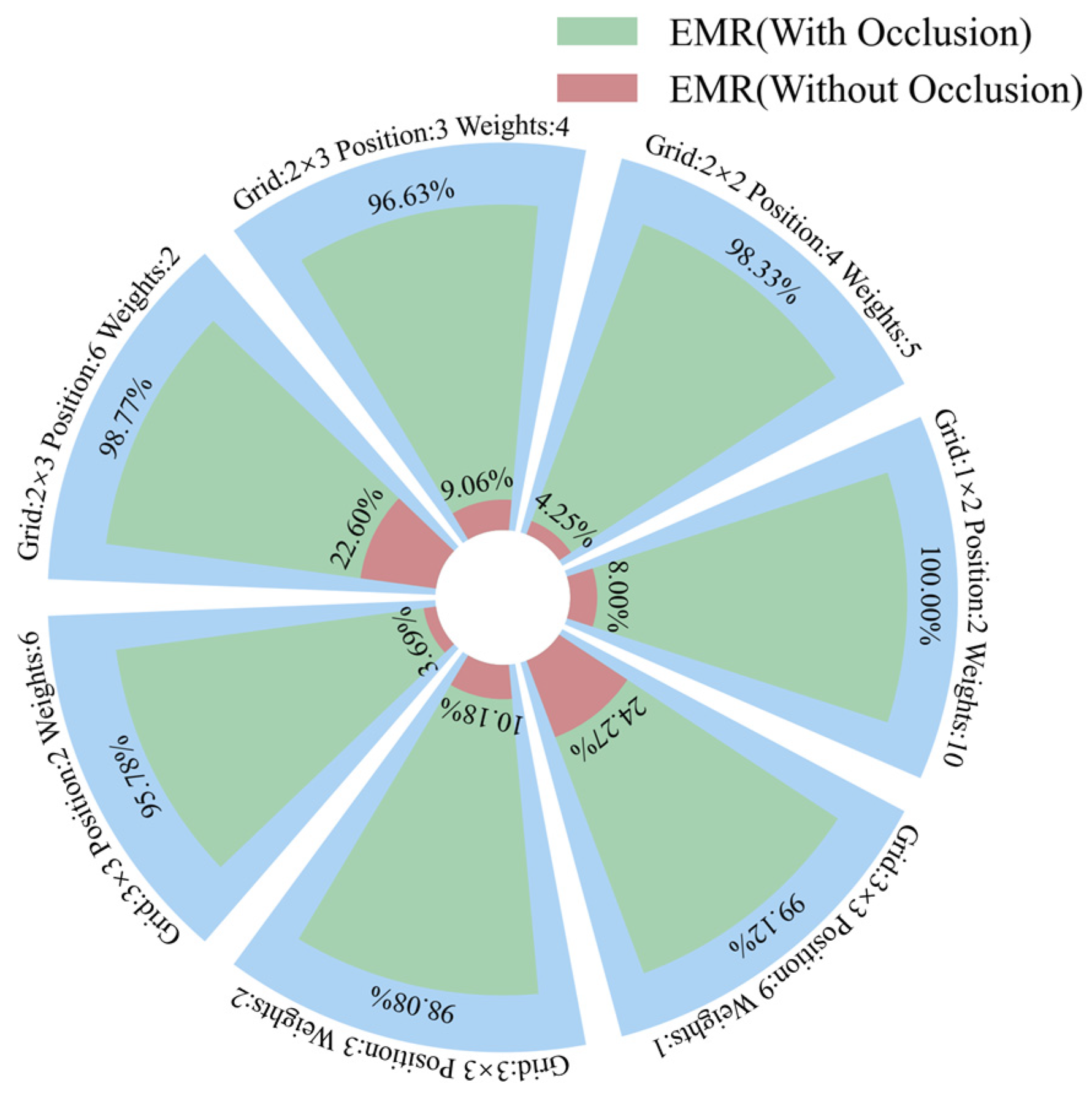
Figure 18.
EMR of shallow CNN on seven datasets.
Figure 18.
EMR of shallow CNN on seven datasets.
Figure 19.
Evaluation metrics of VGG16 with early stopping (early stopping threshold: 10).
Figure 19.
Evaluation metrics of VGG16 with early stopping (early stopping threshold: 10).
Figure 20.
Evaluation metrics of shallow CNN with early stopping (early stopping threshold: 10).
Figure 20.
Evaluation metrics of shallow CNN with early stopping (early stopping threshold: 10).
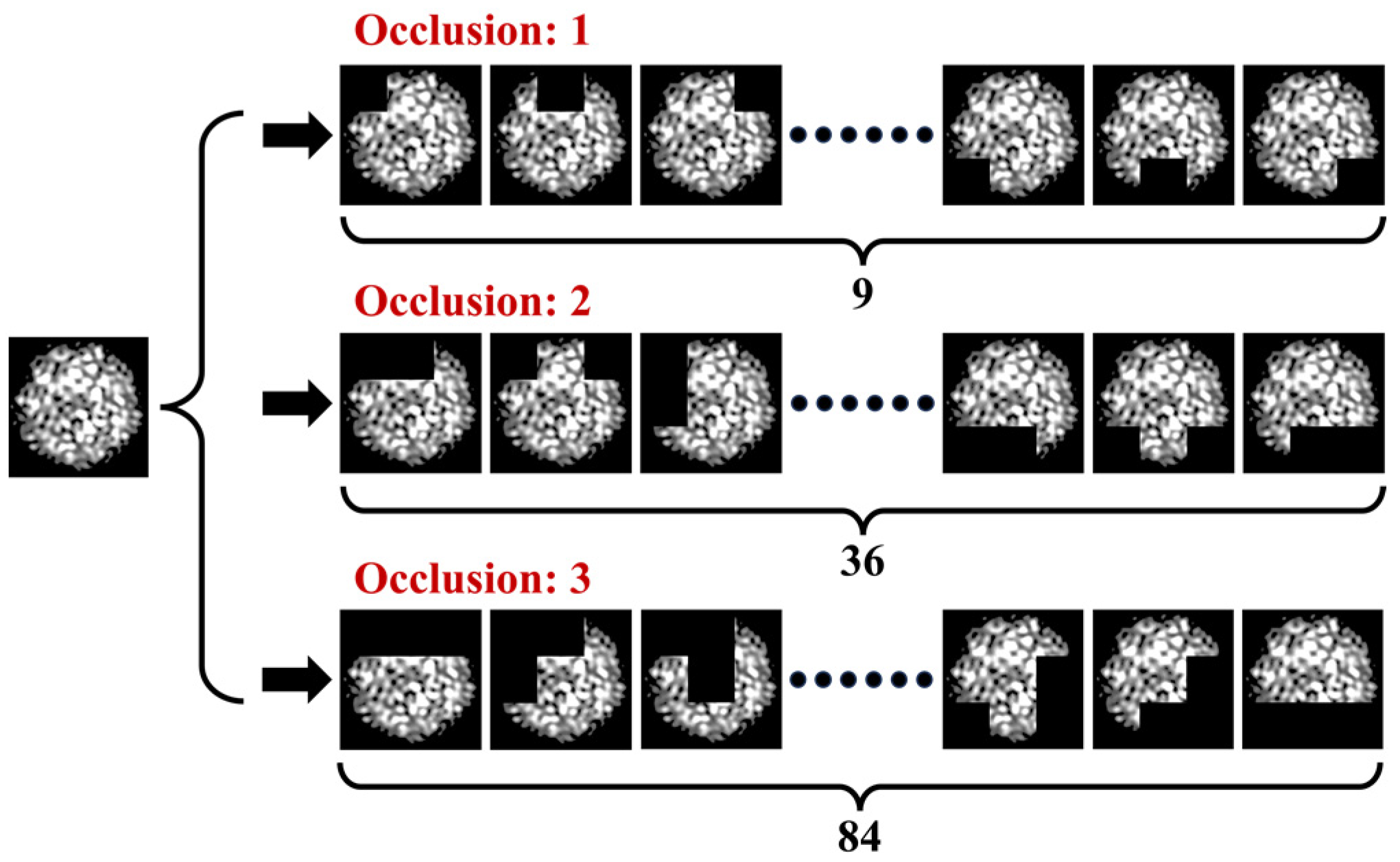
Figure 21.
Diagram illustrating specklegram occlusion generation for analyzing the impact of occlusion count on model convergence speed.
Figure 21.
Diagram illustrating specklegram occlusion generation for analyzing the impact of occlusion count on model convergence speed.
Figure 22.
Model convergence and accuracy of the shallow CNN on various datasets with occlusions of 1–8 and early stopping threshold set to 1 (3 × 3 grid: up to 2 perturbation positions with maximum 15 g load per position).
Figure 22.
Model convergence and accuracy of the shallow CNN on various datasets with occlusions of 1–8 and early stopping threshold set to 1 (3 × 3 grid: up to 2 perturbation positions with maximum 15 g load per position).
Table 1.
The multi-position sensing capability of proposed and existing sensors.
Table 1.
The multi-position sensing capability of proposed and existing sensors.
| Reference | Multi-Position
Sensing Capability | Perturbation Forms | Revolution of Positioning | Accuracy | Multi-Parameter Recognition | Temperature
Compensation |
|---|
| Wei [12] | 10-point positioning | 10 | 60 cm | 92.83% | No (position only) | Transfer learning |
| Cuevas [18] | 3-point and 10-point positioning | 3 and 10 | 120 cm | 99% and 71% | No (position only) | Multi-temperature learning |
| Ding [19] | 9-point positioning | 9 | 0.5 mm | 98% | No (position only) | Multi-temperature learning |
| Sun [20] | 4-direction displacement | 40 | - | 97% | Yes (4 parameters) | Not implemented |
| Fujiwara [21] | 3-point with 3-angle bending | 25 | 0.2 cm | - | Yes (3 parameters) | Correlation analysis |
| Lu [22] | 3-point with 3-angle bending | 27 | 20 cm | 93.5% | Yes (3 parameters) | Not implemented |
| proposed | 6-point with 3 random loads and
9-point with 2 random loads | 1545 and 1351 | 5 cm | 96.63% and 95.78% | Yes (9 parameters) | Transfer learning |
Table 2.
Load combinations of grids.
Table 2.
Load combinations of grids.
| Grid | Maximum Perturbation Positions | Max Weights | Categories |
|---|
| 1 × 2 | 2 | 10 | 121 |
| 2 × 2 | 4 | 5 | 1296 |
| 2 × 3 | 3 | 4 | 1545 |
| 6 | 2 | 729 |
| 3 × 3 | 2 | 6 | 1351 |
| 3 | 2 | 835 |
| 9 | 1 | 512 |
Table 3.
Performance of shallow CNN (without occlusion).
Table 3.
Performance of shallow CNN (without occlusion).
| Grid | Maximum Perturbation
Positions | Max Weights
per Cell | EMR | F1 | Hamming Loss |
|---|
| 1 × 2 | 2 | 10 | 8.00% | 0.4495 | 0.5400 |
| 2 × 2 | 4 | 5 | 4.25% | 0.6553 | 0.5267 |
| 2 × 3 | 3 | 4 | 9.06% | 0.6880 | 0.3031 |
| 6 | 2 | 22.60% | 0.7635 | 0.2352 |
| 3 × 3 | 2 | 6 | 3.69% | 0.7979 | 0.1812 |
| 3 | 2 | 10.18% | 0.7724 | 0.2102 |
| 9 | 1 | 24.27% | 0.8405 | 0.1597 |
Table 4.
Performance of shallow CNN (with occlusion).
Table 4.
Performance of shallow CNN (with occlusion).
| Grid | Maximum Perturbation
Positions | Max Weights
per Cell | EMR | F1 | Hamming Loss |
|---|
| 1 × 2 | 2 | 10 | 100% | 1 | 0 |
| 2 × 2 | 4 | 5 | 98.33% | 0.9985 | 0.0019 |
| 2 × 3 | 3 | 4 | 96.63% | 0.9942 | 0.0058 |
| 6 | 2 | 98.77% | 0.9977 | 0.0023 |
| 3 × 3 | 2 | 6 | 95.78% | 0.9951 | 0.0048 |
| 3 | 2 | 98.08% | 0.9977 | 0.0023 |
| 9 | 1 | 99.12% | 0.9990 | 0.0010 |
Table 5.
Performance of the different models on 1 × 2 grid (up to 2 perturbation positions with maximum 50 g load per cell).
Table 5.
Performance of the different models on 1 × 2 grid (up to 2 perturbation positions with maximum 50 g load per cell).
| Method | Model | EMR | F1 | Hamming |
|---|
| Without occlusion | VGG16 | 4.00% | 0.3853 | 0.6000 |
| ResNet-18 | 0.00% | 0.3401 | 0.6400 |
| CNN-Shallow | 8.00% | 0.4495 | 0.5400 |
| With occlusion | VGG16 | 96.69% | 0.9829 | 0.0165 |
| ResNet-18 | 100% | 1 | 0 |
| CNN-Shallow | 100% | 1 | 0 |
Table 6.
Performance of the different models on 3 × 3 grid (up to 2 perturbation positions with maximum 15 g load per cell).
Table 6.
Performance of the different models on 3 × 3 grid (up to 2 perturbation positions with maximum 15 g load per cell).
| Method | Model | EMR | F1 | Hamming |
|---|
| Without occlusion | VGG16 | 4.53% | 0.6453 | 0.3350 |
| ResNet-18 | 0.97% | 0.5065 | 0.4358 |
| CNN-Shallow | 9.06% | 0.6880 | 0.3031 |
| With occlusion | VGG16 | 98.25% | 0.9978 | 0.0029 |
| ResNet-18 | 98.06% | 0.9967 | 0.0033 |
| CNN-Shallow | 96.63% | 0.9942 | 0.0058 |
Table 7.
Performance of the different models on 3 × 3 grid (up to 9 perturbation positions with maximum 5 g load per cell).
Table 7.
Performance of the different models on 3 × 3 grid (up to 9 perturbation positions with maximum 5 g load per cell).
| Method | Model | EMR | F1 | Hamming |
|---|
| Without occlusion | VGG16 | 0% | 0.7569 | 0.2254 |
| ResNet-18 | 0% | 0.7093 | 0.2050 |
| CNN-Shallow | 4.225% | 0.7696 | 0.1753 |
| With occlusion | VGG16 | 100% | 1 | 0 |
| ResNet-18 | 100% | 1 | 0 |
| CNN-Shallow | 100% | 1 | 0 |
Table 8.
Performance of the different models on 2 × 3 grid (up to 3 perturbation positions with maximum 20 g load per cell).
Table 8.
Performance of the different models on 2 × 3 grid (up to 3 perturbation positions with maximum 20 g load per cell).
| Method | Model | EMR | F1 | Hamming |
|---|
| Without occlusion | VGG16 | 9.71% | 0.7718 | 0.2276 |
| ResNet-18 | 1.94% | 0.6466 | 0.3528 |
| CNN-Shallow | 24.27% | 0.8405 | 0.1597 |
| With occlusion | VGG16 | 99.41% | 0.9993 | 0.0007 |
| ResNet-18 | 98.93% | 0.9988 | 0.0012 |
| CNN-Shallow | 99.12% | 0.9990 | 0.0010 |
Table 9.
Training performance of the different models with early stopping (3 × 3 grid: up to 2 perturbation positions with maximum 15 g load per cell).
Table 9.
Training performance of the different models with early stopping (3 × 3 grid: up to 2 perturbation positions with maximum 15 g load per cell).
| Early Stopping Threshold | Model | Epoch | Training Time (s) |
|---|
| 10 | VGG16 | 705 | 40,947.79 |
| ResNet-18 | 783 | 1195.05 |
| CNN-Shallow | 296 | 134.18 |
| 3 | VGG16 | 250 | 15,460.77 |
| ResNet-18 | 765 | 1170.18 |
| CNN-Shallow | 282 | 130.28 |
| 1 | VGG16 | 122 | 7147.60 |
| ResNet-18 | 641 | 978.46 |
| CNN-Shallow | 268 | 121.32 |
Table 10.
Performance of the shallow CNN on various datasets with occlusions of 1–8 and an early stopping threshold set to 1 (3 × 3 grid: up to 2 perturbation positions with maximum 15 g load per position).
Table 10.
Performance of the shallow CNN on various datasets with occlusions of 1–8 and an early stopping threshold set to 1 (3 × 3 grid: up to 2 perturbation positions with maximum 15 g load per position).
| Occlusions | Epoch | EMR | Training Time (s) |
|---|
| 1 | 268 | 100% | 120.59 |
| 2 | 124 | 100% | 198.37 |
| 3 | 62 | 100% | 229.57 |
| 4 | 130 | 100% | 686.22 |
| 5 | 1000 | 99.98% | 5374.29 |
| 6 | 1000 | 99.08% | 3583.20 |
| 7 | 1000 | 91.93% | 1548.42 |
| 8 | 1000 | 14.91% | 440.12 |
Table 11.
Performance of the difference grids and early stopping threshold set to 1 (up to 2 perturbation positions with maximum 15 g load per position).
Table 11.
Performance of the difference grids and early stopping threshold set to 1 (up to 2 perturbation positions with maximum 15 g load per position).
| Grids of Specklegram | Epoch | EMR | Training Time (s) | Dataset Loading Time (s) |
|---|
| 2 × 2 | 1000 | 91.19% | 242.89 | 15.82 |
| 3 × 3 | 268 | 100% | 120.59 | 49.23 |
| 4 × 4 | 163 | 100% | 125.85 | 55.19 |
| 5 × 5 | 87 | 100% | 105.04 | 83.68 |
| 6 × 6 | 76 | 100% | 128.78 | 119.58 |
| 7 × 7 | 53 | 100% | 122.18 | 161.13 |
Table 12.
Specklegram datasets under different temperatures (3 × 3 grid: up to 2 perturbation positions with maximum 15 g load per position).
Table 12.
Specklegram datasets under different temperatures (3 × 3 grid: up to 2 perturbation positions with maximum 15 g load per position).
| Dataset | Temperature/°C |
|---|
| 1 | 20.9 |
| 2 | 21.1 |
| 3 | 21.3 |
| 4 | 21.3 |
| 5 | 21.2 |
| 6 | 22.4 |
| 7 | 22.2 |
| 8 | 21.9 |
| 9 | 21.7 |
| 10 | 21.5 |
Table 13.
Recognition EMR of Models 1-5 for each dataset (3 × 3 grid: up to 2 perturbation positions with maximum 15 g load per position).
Table 13.
Recognition EMR of Models 1-5 for each dataset (3 × 3 grid: up to 2 perturbation positions with maximum 15 g load per position).
| Occlusion Grid | Model | EMR of Dataset |
|---|
| 1 | 2 | 3 | 4 | 5 | 6 | 7 | 8 | 9 | 10 |
|---|
| 3 × 3 | 1 | 100% | 3.12% | 0.85% | 0.28% | 0.00% | 0.28% | 0.57% | 0.28% | 0.28% | 0.57% |
| 2 | 100% | 100% | 100% | 100% | 100% | 0.57% | 0.28% | 0.00% | 0.57% | 0.00% |
| 3 | 100% | 14.77% | 100% | 8.81% | 100% | 4.26% | 100% | 16.76% | 100% | 8.81% |
| 4 | 100% | 46.02% | 47.73% | 42.33% | 38.92% | 37.50% | 45.74% | 43.18% | 43.18% | 40.34% |
| 5 | 100% | 68.18% | 69.32% | 67.61% | 62.50% | 63.64% | 68.47% | 69.32% | 69.89% | 67.61% |
| 5 × 5 | 1 | 100% | 3.69% | 0.85% | 0.28% | 0.28% | 0.28% | 0.57% | 0.28% | 0.28% | 0.85% |
| 2 | 100% | 100% | 100% | 100% | 100% | 0.57% | 0.57% | 0.28% | 0.57% | 0.00% |
| 3 | 100% | 10.23% | 100% | 8.81% | 100% | 5.40% | 100% | 16.48% | 100% | 9.38% |
| 4 | 100% | 79.83% | 78.12% | 76.14% | 76.99% | 71.88% | 80.68% | 80.11% | 79.55% | 74.43% |
| 5 | 100% | 95.17% | 92.33% | 93.47% | 94.89% | 93.18% | 96.31% | 94.60% | 96.31% | 93.18% |


