
An Inversion Model for Suspended Sediment Concentration Based on Hue Angle Optical Classification: A Case Study of the Coastal Waters in the Guangdong-Hong Kong-Macao Greater Bay Area

 , , and
Abstract
1. Introduction
2. Methodology
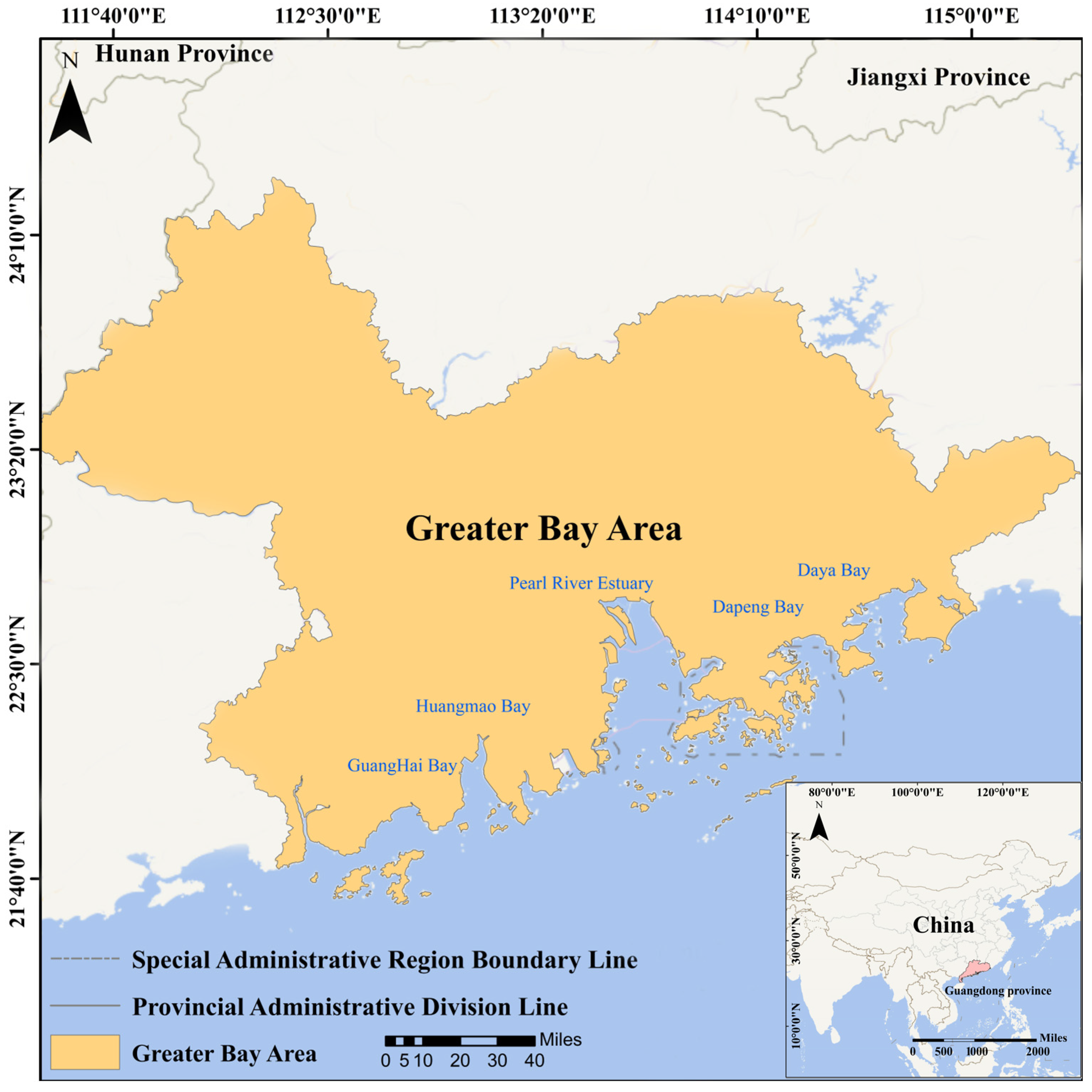
2.1. Study Area
2.2. Study Data
2.3. Landsat8 OLI Image Processing
2.4. Water Optical Classification
2.5. Model Construction
2.6. Spatial Analysis
2.7. Accuracy Metrics
3. Result
3.1. Comparison Between Hue Angle and SSC Values
3.2. Validation of the SSC Inversion Model
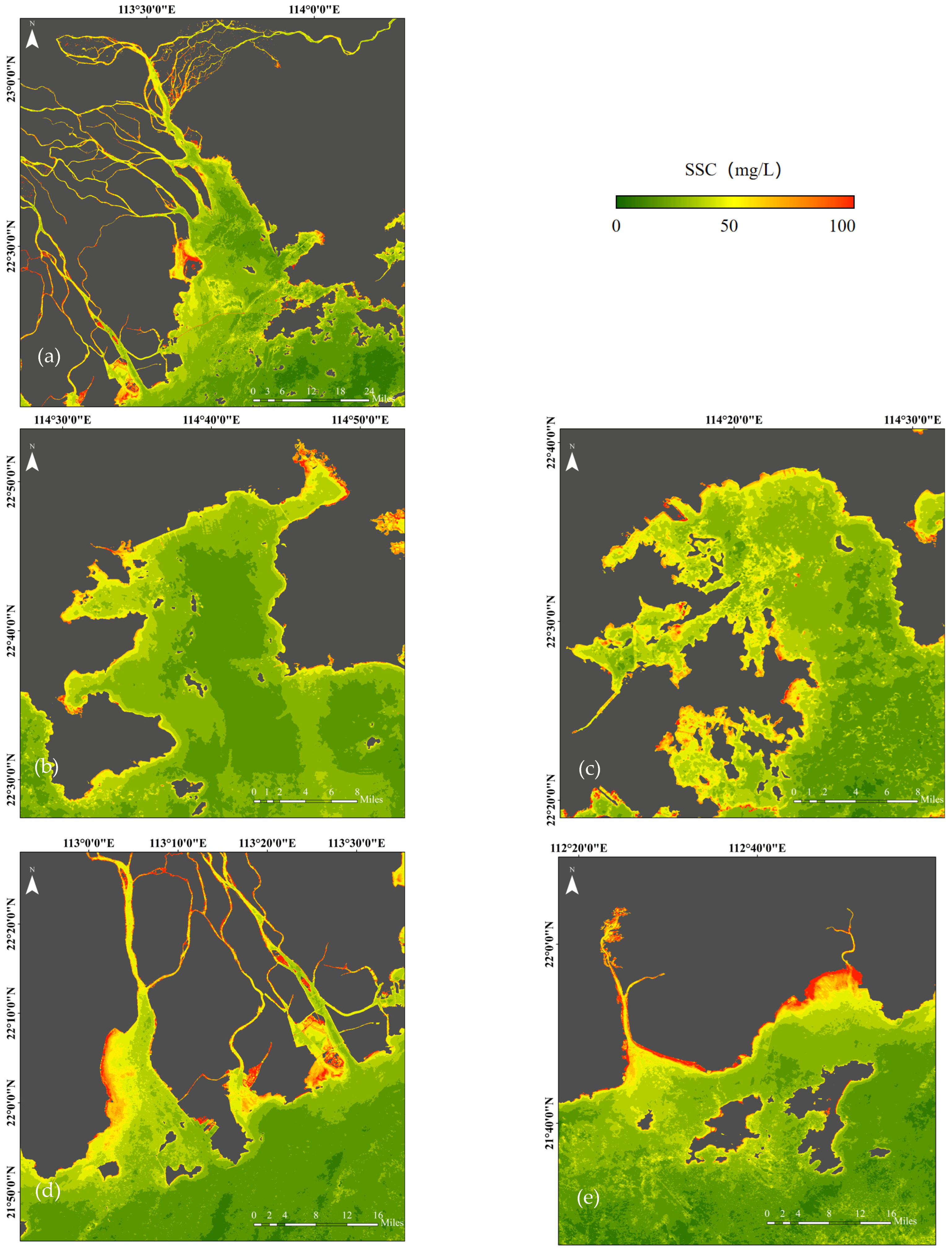
3.3. Spatiotemporal Analysis of SSC in the Greater Bay Area
4. Discussion
4.1. Comparison of SSC Inversion Models
4.2. Uncertainty Analysis
5. Conclusions
Supplementary Materials
Author Contributions
Funding
Data Availability Statement
Acknowledgments
Conflicts of Interest
References
- Xiao, Y.; Wu, Z.; Cai, H.; Tang, H. Suspended Sediment Dynamics in a Well-Mixed Estuary: The Role of High Suspended Sediment Concentration (SSC) from the Adjacent Sea Area. Estuar. Coast Shelf Sci. 2018, 209, 191–204. [Google Scholar] [CrossRef]
- Zhou, T.; Cao, B.; Qiu, J.; Cai, S.; Ou, H.; Fan, W.; Yang, X.; Xie, X.; Bo, Y.; Zhang, G. Mapping Suspended Sediment Changes in the Western Pacific Coasts. Remote Sens. 2023, 15, 5192. [Google Scholar] [CrossRef]
- Adjovu, G.E.; Stephen, H.; James, D.; Ahmad, S. Measurement of Total Dissolved Solids and Total Suspended Solids in Water Systems: A Review of the Issues, Conventional, and Remote Sensing Techniques. Remote Sens. 2023, 15, 3534. [Google Scholar] [CrossRef]
- Tian, T.; Merico, A.; Su, J.; Staneva, J.; Wiltshire, K.; Wirtz, K. Importance of Resuspended Sediment Dynamics for the Phytoplankton Spring Bloom in a Coastal Marine Ecosystem. J. Sea Res. 2009, 62, 214–228. [Google Scholar] [CrossRef]
- Liu, X.; Wang, Y.; Zhang, Q.; Liu, C.; Song, Y.; Li, Y.; Yin, Y.; Cai, Y. Confounding Effects of Seasonality and Anthropogenic River Regulation on Suspended Particulate Matter-Driven Mercury Transport to Coastal Seas. J. Hazard Mater. 2024, 469, 133979. [Google Scholar] [CrossRef]
- Liu, X.; Sheng, Y.; Liu, Q.; Li, Z. Suspended Particulate Matter Affects the Distribution and Migration of Heavy Metals in the Yellow River. Sci. Total Environ. 2024, 912, 169537. [Google Scholar] [CrossRef]
- Glasgow, H.B.; Burkholder, J.A.M.; Reed, R.E.; Lewitus, A.J.; Kleinman, J.E. Real-Time Remote Monitoring of Water Quality: A Review of Current Applications, and Advancements in Sensor, Telemetry, and Computing Technologies. J. Exp. Mar. Biol. Ecol. 2004, 300, 409–448. [Google Scholar] [CrossRef]
- Bai, X.; Wang, J.; Chen, R.; Kang, Y.; Ding, Y.; Lv, Z.; Ding, D.; Feng, H. Research Progress of Inland River Water Quality Monitoring Technology Based on Unmanned Aerial Vehicle Hyperspectral Imaging Technology. Environ. Res. 2024, 257, 119–254. [Google Scholar] [CrossRef]
- Mutunga, T.; Sinanovic, S.; Harrison, C.S. Integrating Wireless Remote Sensing and Sensors for Monitoring Pesticide Pollution in Surface and Groundwater. Sensors 2024, 24, 3191. [Google Scholar] [CrossRef]
- Cai, L.; Zhou, M.; Liu, J.; Tang, D.; Zuo, J. HY-1C Observations of the Impacts of Islands on Suspended Sediment Distribution in Zhoushan Coastal Waters, China. Remote Sens. 2020, 12, 1766. [Google Scholar] [CrossRef]
- Marinho, R.R.; Harmel, T.; Martinez, J.M.; Junior, N.P.F. Spatiotemporal Dynamics of Suspended Sediments in the Negro River, Amazon Basin, from in Situ and Sentinel-2 Remote Sensing Data. ISPRS Int. J. Geoinf. 2021, 10, 86. [Google Scholar] [CrossRef]
- Larson, M.D.; Simic Milas, A.; Vincent, R.K.; Evans, J.E. Landsat 8 Monitoring of Multi-Depth Suspended Sediment Concentrations in Lake Erie’s Maumee River Using Machine Learning. Int. J. Remote Sens. 2021, 42, 4064–4086. [Google Scholar] [CrossRef]
- Zhao, G.; Jiang, W.; Wang, T.; Chen, S.; Bian, C. Decadal Variation and Regulation Mechanisms of the Suspended Sediment Concentration in the Bohai Sea, China. J. Geophys. Res. Oceans 2022, 127. [Google Scholar] [CrossRef]
- Bernardo, N.; do Carmo, A.; Park, E.; Alc’ntara, E. Retrieval of Suspended Particulate Matter in Inland Waters with Widely Differing Optical Properties Using a Semi-Analytical Schemee. Remote Sens. 2019, 11, 2283. [Google Scholar] [CrossRef]
- Dang, X.; Du, J.; Wang, C.; Zhang, F.; Wu, L.; Liu, J.; Wang, Z.; Yang, X.; Wang, J. A Hybrid Chlorophyll a Estimation Method for Oligotrophic and Mesotrophic Reservoirs Based on Optical Water Classification. Remote Sens. 2023, 15, 2209. [Google Scholar] [CrossRef]
- Nasir, N.; Kansal, A.; Alshaltone, O.; Barneih, F.; Sameer, M.; Shanableh, A.; Al-Shamma’a, A. Water Quality Classification Using Machine Learning Algorithms. J. Water Process Eng. 2022, 48, 102920. [Google Scholar] [CrossRef]
- Vantrepotte, V.; Loisel, H.; Dessailly, D.; Mériaux, X. Optical Classification of Contrasted Coastal Waters. Remote Sens. Environ. 2012, 123, 306–323. [Google Scholar] [CrossRef]
- Mao, Z.; Chen, J.; Pan, D.; Tao, B.; Zhu, Q. A Regional Remote Sensing Algorithm for Total Suspended Matter in the East China Sea. Remote Sens. Environ. 2012, 124, 819–831. [Google Scholar] [CrossRef]
- Balasubramanian, S.V.; Pahlevan, N.; Smith, B.; Binding, C.; Schalles, J.; Loisel, H.; Gurlin, D.; Greb, S.; Alikas, K.; Randla, M.; et al. Robust Algorithm for Estimating Total Suspended Solids (TSS) in Inland and Nearshore Coastal Waters. Remote Sens. Environ. 2020, 246, 111768. [Google Scholar] [CrossRef]
- Calvario Sanchez, G.; Dalmau, O.; Alarcon, T.E.; Sierra, B.; Hernandez, C. Selection and Fusion of Spectral Indices to Improve Water Body Discrimination. IEEE Access 2018, 6, 72952–72961. [Google Scholar] [CrossRef]
- Wernand, M.R.; Hommersom, A.; Van Der Woerd, H.J. MERIS-Based Ocean Colour Classification with the Discrete Forel-Ule Scale. Ocean Sci. 2013, 9, 477–487. [Google Scholar] [CrossRef]
- Liu, Y.; Wu, H.; Wang, S.; Chen, X.; Kimball, J.S.; Zhang, C.; Gao, H.; Guo, P. Evaluation of Trophic State for Inland Waters through Combining Forel-Ule Index and Inherent Optical Properties. Sci. Total Environ. 2022, 820, 153316. [Google Scholar] [CrossRef] [PubMed]
- Zhang, C.; Liu, Y.; Chen, X.; Gao, Y. Estimation of Suspended Sediment Concentration in the Yangtze Main Stream Based on Sentinel-2 MSI Data. Remote Sens. 2022, 14, 4446. [Google Scholar] [CrossRef]
- Vanhellemont, Q.; Ruddick, K. Atmospheric Correction of Metre-Scale Optical Satellite Data for Inland and Coastal Water Applications. Remote Sens. Environ. 2018, 216, 586–597. [Google Scholar] [CrossRef]
- Vanhellemont, Q. Adaptation of the Dark Spectrum Fitting Atmospheric Correction for Aquatic Applications of the Landsat and Sentinel-2 Archives. Remote Sens. Environ. 2019, 225, 175–192. [Google Scholar] [CrossRef]
- Cox, C.; Munk, W. Measurement of the Roughness of the Sea Surface from Photographs of the Sun’s Glitter. J. Opt. Soc. Am. 1954, 44, 838–850. [Google Scholar] [CrossRef]
- Wang, S.; Li, J.; Zhang, B.; Lee, Z.; Spyrakos, E.; Feng, L.; Liu, C.; Zhao, H.; Wu, Y.; Zhu, L.; et al. Changes of Water Clarity in Large Lakes and Reservoirs across China Observed from Long-Term MODIS. Remote Sens. Environ. 2020, 247, 111949. [Google Scholar] [CrossRef]
- van der Woerd, H.J.; Wernand, M.R. Hue-Angle Product for Low to Medium Spatial Resolution Optical Satellite Sensors. Remote Sens. 2018, 10, 180. [Google Scholar] [CrossRef]
- Li, J.; Zhang, W.; Deng, R.; Lu, Z.; Liang, Y.; Shen, X.; Xiong, L.; Liu, Y. The Study of Spatial-Temporal Characteristics for CODMn in Shenzhen Reservoir Based on GF-1 WFV. J. Remote Sens. 2022, 26, 1562–1574. [Google Scholar] [CrossRef]
- Wan, Y.; Wang, L. Numerical Investigation of the Factors Influencing the Vertical Profiles of Current, Salinity, and SSC within a Turbidity Maximum Zone. Int. J. Sediment Res. 2017, 32, 20–33. [Google Scholar] [CrossRef]
- Cao, B.; Qiu, J.; Zhang, W.; Xie, X.; Lu, X.; Yang, X.; Li, H. Retrieval of Suspended Sediment Concentrations in the Pearl River Estuary Using Multi-Source Satellite Imagery. Remote Sens. 2022, 14, 3896. [Google Scholar] [CrossRef]
- Yue, Y.; Qing, S.; Diao, R.; Hao, Y. Remote Sensing of Suspended Particulate Matter in Optically Complex Estuarine and Inland Waters Based on Optical Classification. J. Coast. Res. 2020, 102, 303–317. [Google Scholar] [CrossRef]
- Yu, D.; Bian, X.; Yang, L.; Zhou, Y.; An, D.; Zhou, M.; Chen, S.; Pan, S. Monitoring Suspended Sediment Concentration in the Yellow River Estuary from 1984 to 2021 Using Landsat Imagery and Google Earth Engine. Int. J. Remote Sens. 2023, 44, 3122–3145. [Google Scholar] [CrossRef]
- Kaufman, Y.J.; Tanré, D.; Gordon, H.R.; Nakajima, T.; Lenoble, J.; Frouin, R.; Grassl, H.; Herman, B.M.; King, M.D.; Teillet, P.M. Passive Remote Sensing of Tropospheric Aerosol and Atmospheric Correction for the Aerosol Effect. J. Geophys. Res. Atmos. 1997, 102, 16815–16830. [Google Scholar] [CrossRef]
- Li, H.; He, X.; Shanmugam, P.; Bai, Y.; Wang, D.; Huang, H.; Zhu, Q.; Gong, F. Radiometric Sensitivity and Signal Detectability of Ocean Color Satellite Sensor under High Solar Zenith Angles. IEEE Trans. Geosci. Remote Sens. 2019, 57, 8492–8505. [Google Scholar] [CrossRef]
- Pereira-Sandoval, M.; Ruescas, A.; Urrego, P.; Ruiz-Verdú, A.; Delegido, J.; Tenjo, C.; Soria-Perpinyà, X.; Vicente, E.; Soria, J.; Moreno, J. Evaluation of Atmospheric Correction Algorithms over Spanish Inland Waters for Sentinel-2 Multi Spectral Imagery Data. Remote Sens. 2019, 11, 1469. [Google Scholar] [CrossRef]
- Mohseni, F.; Saba, F.; Mirmazloumi, S.M.; Amani, M.; Mokhtarzade, M.; Jamali, S.; Mahdavi, S. Ocean Water Quality Monitoring Using Remote Sensing Techniques: A Review. Mar. Environ. Res. 2022, 180, 105701. [Google Scholar] [CrossRef]


| Dataset | Number | Max (mg/L) | Min (mg/L) | Mean (mg/L) |
|---|---|---|---|---|
| Sampling data | 43 | 36 | 0.6 | 13.71 |
| GPDEE data | 654 | 263.1 | 0.3 | 9.36 |
| HKEPD data | 4234 | 360 | 0.5 | 8.15 |
| HBGP | 86 | 173 | 1.2 | 10.08 |
| Total | 5017 | 360 | 0.3 | 8.65 |
| Model | R2 | RMSE | MAPE |
|---|---|---|---|
| Single-Scattering | 0.60 | 10.11 | 44.09% |
| Secondary-Scattering | 0.71 | 8.38 | 45.47% |
| Angle-SS | 0.73 | 8.30 | 42.00% |
| Model | Model Form | RMSE | MAPE |
|---|---|---|---|
| Yu [33] | SSC = 0.8079 × BRed/BGreen + 23.062 × BNIR + 0.6258 | 11.55 | 79.57% |
| Cao [31] | SSC = 3.501 × e4.317 × Rrs | 10.65 | 60.39% |
| Yue [32] | lnSSCclass1 = 65.011 × Rrs665 − 2.243 × Rrs740/Rrs665 + 4.09 × Rrs705/Rrs665 − 0.449, MCI ≤ 0.0016 lnSSCclass1 = −30.941 × Rrs740 − 2.667 × Rrs740/Rrs492 + 3.224, MCI ≤ 0.0016 (MCI: maximum chlorophyll index) | 9.85 | 52.36% |
| This study | - | 8.30 | 42.00% |
Disclaimer/Publisher’s Note: The statements, opinions and data contained in all publications are solely those of the individual author(s) and contributor(s) and not of MDPI and/or the editor(s). MDPI and/or the editor(s) disclaim responsibility for any injury to people or property resulting from any ideas, methods, instructions or products referred to in the content. |
© 2025 by the authors. Licensee MDPI, Basel, Switzerland. This article is an open access article distributed under the terms and conditions of the Creative Commons Attribution (CC BY) license (https://creativecommons.org/licenses/by/4.0/).
Share and Cite
Yang, J.; Deng, R.; Ma, Y.; Li, J.; Guo, Y.; Lei, C. An Inversion Model for Suspended Sediment Concentration Based on Hue Angle Optical Classification: A Case Study of the Coastal Waters in the Guangdong-Hong Kong-Macao Greater Bay Area. Sensors 2025, 25, 1728. https://doi.org/10.3390/s25061728
Yang J, Deng R, Ma Y, Li J, Guo Y, Lei C. An Inversion Model for Suspended Sediment Concentration Based on Hue Angle Optical Classification: A Case Study of the Coastal Waters in the Guangdong-Hong Kong-Macao Greater Bay Area. Sensors. 2025; 25(6):1728. https://doi.org/10.3390/s25061728
Chicago/Turabian StyleYang, Junying, Ruru Deng, Yiwei Ma, Jiayi Li, Yu Guo, and Cong Lei. 2025. "An Inversion Model for Suspended Sediment Concentration Based on Hue Angle Optical Classification: A Case Study of the Coastal Waters in the Guangdong-Hong Kong-Macao Greater Bay Area" Sensors 25, no. 6: 1728. https://doi.org/10.3390/s25061728
APA StyleYang, J., Deng, R., Ma, Y., Li, J., Guo, Y., & Lei, C. (2025). An Inversion Model for Suspended Sediment Concentration Based on Hue Angle Optical Classification: A Case Study of the Coastal Waters in the Guangdong-Hong Kong-Macao Greater Bay Area. Sensors, 25(6), 1728. https://doi.org/10.3390/s25061728